Study of NVIS Channel for USN Protocol Definition in Antarctica

Abstract

Every year, the number of ubiquitous sensor networks (USN) is increasing and the need for remote USN communications is emerging in some scenarios. As an alternative to satellite communications, more interests are focused on high frequencies (HF) communications as a low-cost option to reach links of more than 250 km without a line of sight. The HF standards are designed for generic communication channels being not robust for near vertical incidence skywave (NVIS) USN. In this article, we propose a new protocol for USN in remote places based on NVIS communications. For that purpose, we study the main characteristics of the NVIS channel with the presence of groundwaves, particularly in Antarctica. We analyze the availability of the channel, the height of the layers, the delay spread, and the Doppler spread. On the basis of the results obtained, we propose two protocols based on an OFDM (orthogonal frequency division multiplexing) modulation depending on the presence of the groundwave at the receiver. Finally, we make a simulation of the two OFDM configurations and we compare it with real tested standard modulations. The results show a better performance of the new protocol compared to the current HF standards.

1. Introduction

Nowadays the number of connected devices as ubiquitous sensor networks (USN) has increased significantly compared to previous years. The number of Internet of Things (IoT) devices connected in 2019 was about 26.66 billion and is expected to increase up to 75.44 billion of devices at 2025 [1]. This fact is directly related to the appearance of new technologies and frame protocols to connect those devices according to their needs. For example, the use of NB-IoT and LTE-M achieves an easy connectivity by taking advantage of the 3G and 4G networks. On the other hand, Sigfox [2] and LoRa Alliance [3] have defined new frame protocols and frequency usage to maximize the connectivity distance and the number of devices connected to one node. In the same way, Wize Alliance [4] defined the frequency usage to achieve a high penetration on walls to assure the connectivity in meters rooms or basements.

In the same vein, many studies to improve the wireless frame protocols for ubiquitous sensor network (USN) are currently under way as we can see in [5], and studies of long range communications for USN are growing as we can see in [6]. Moreover, high frequency (HF) communications are emerging as a promising alternative to satellite connections for remote internet of things (RIoT) because of their special propagation characteristics. In places without any telecommunication infrastructure, the reflection of the wave in the ionosphere with an oblique incidence angle between 0° and 70°, yields to establish communications up to 12,000 km without line of sight [7,8,9,10,11]. Furthermore, the reflection of the wave in the ionosphere with a vertical incidence angle between 70° and 90°, allows communications up to 250 km without a line of sight [12]. This is called near vertical incidence skywave (NVIS) and the usable frequencies range from 3 MHz to 10 MHz. As the power transmission is low, typically below 10 W, it is a good option for RIoT in locations without an electrical network with a self-sufficient energy system. On the other hand, the maximum of the radiation diagram must be upward, large horizontal dipoles and inverted-V antennas are commonly used with masts up to 15 m high. However, we can also use smaller antennas such as loops if we keep the antenna losses under control. Although the power transmission is low and the antenna gain is negative, the use of low consumption NVIS communications for USN becomes feasible since the losses due to obstacles are negligible. Even in the presence of mountains in between, the free space propagation losses are the only ones to be taken into account [13]. However, NVIS low power transmissions cannot reach high bitrates as 3G and 4G networks. In this case, the bandwidth usage is about 3 kHz to obtain bitrates of 6 Kbps as maximum [14], which is enough for most USN.

Actually, we can find some previous works related to the improvement of the ionospheric communications based on the analysis of the ionospheric channel, polarization techniques, narrowband modulations, and multicarrier modulations.

Jodalen [15], Hervas [16], Cannon [17] and Warrington [18] study the main characteristics of the NVIS channel as the availability, delay spread, Doppler spread, and Doppler shift for 3 kHz transmissions. In our work, we will study the main characteristics of the NVIS channel and by the analysis of it, we will design a new NVIS frame protocol.

Li [19] and Erhel [20] study different polarization ways to receive the NVIS signal with the purpose of applying by multiple input multiple output (MIMO) polarization techniques to improve the transmissions. In our work, we focused the study on the improvement of the transmissions by the redefinition of the frame protocol.

In addition, Ismail [21] studies narrowband modulations with 3 kHz of bandwidth to analyse the performance of each modulation. In our work, we compare the robustness of two narrowband modulations real tested in comparison to a multicarrier modulation designed taking into account the NVIS channel effects measured.

Bergada [22] studies a comparison between spread spectrum and multicarrier modulations based on previous studies of a long haul HF channel effects. In our work, we compare a multicarrier modulation with narrowband modulations based on a study done in this work of the NVIS channel effects. Also in this article, we propose a new frame protocol to improve the communication.

At last, Antoniou [23] studies the improvement of the data rate transmission on a 3 kHz NVIS channel by the use of differential modulations. In contrast, our work will be focused on the improvement of the robustness of the transmission instead of the data rate.

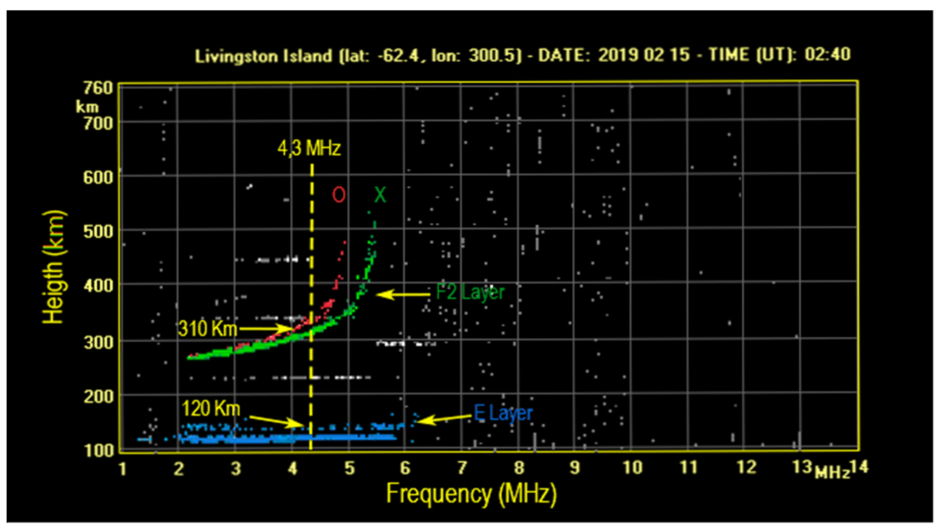
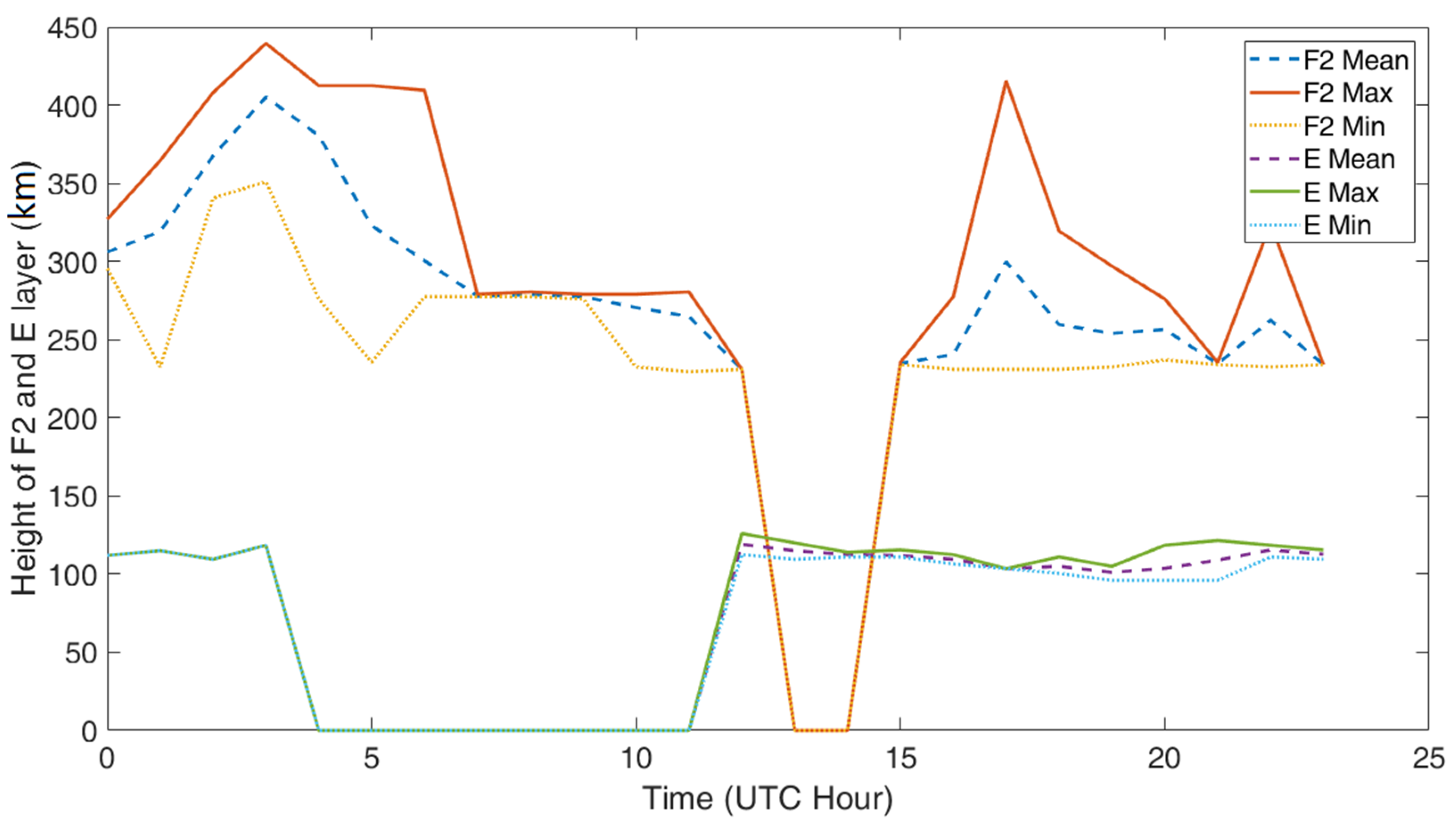
The HF communications frame protocols are defined at STANAG [24] and MIL-STD 188 110C Appendix D [25]. These HF communication frame protocols are designed for both oblique and NVIS communications which have different channel parameters. The NVIS communications can communicate from 0 km to 250 km and oblique communications more than 250 km. For short distances, depending on the terrain, depending on the terrain, the groundwave can be received. In contrast to the skywave, the groundwave is a wave which is propagated by the surface of the terrain. For distances shorter than 10 km you may receive both the groundwave and the skywave, which can be studied separately and will cause multipath interference. For vertical incidence, the sporadic-E layer often appears together with the F2 layer and also causes multipath interference [26]. In oblique communications the interferences produced by multiple paths are lower than NVIS communications.

In this article, we study the main characteristics of the NVIS channel for high latitudes, particularly in Antarctica. The new frame protocol definition will be focused on the requirements of USN in remote areas based on NVIS communications with an electromagnetic coverage area from 0 km to 250 km. Although NVIS communications at distances between 0 km and 10 km are not normally used, there may be cases where several nodes can be distributed around the principal node from distances between 0 km and 250 km. This scenario case is the one we tested to define a new frame protocol. The groundwave may be received for short distances without a line of sight, making the correct reception much harder. The current frame protocols do not consider this distance making very complex the reception of a message. For this reason, the purpose of this study is to define a frame protocol based on an orthogonal frequency division multiplexing (OFDM) modulation instead of the actual modulations used at the HF standards. The OFDM modulation will assure at all the communication of the USN. The definition of this frame protocol is set depending on the characteristics of different NVIS channel situations. We measure the Doppler shift and the delay spread of the channel [27] for both the groundwave, sporadic-E layer and F2 layer as a function of time in an NVIS area around the Spanish Antarctic Base Juan Carlos I in Livingston Island.

This article is organized as follows. In Section 2, we detail the test location, the system used to perform the channel tests and the frame structure used. In Section 3, we describe the analysis signal processing to obtain the results and we show the NVIS channel results obtained. In Section 4, based on the results obtained, we explain the proposed frame protocol and the differences with the actual HF standards. Finally, Section 5 contains the conclusions achieved in this article.

2. Sounding System

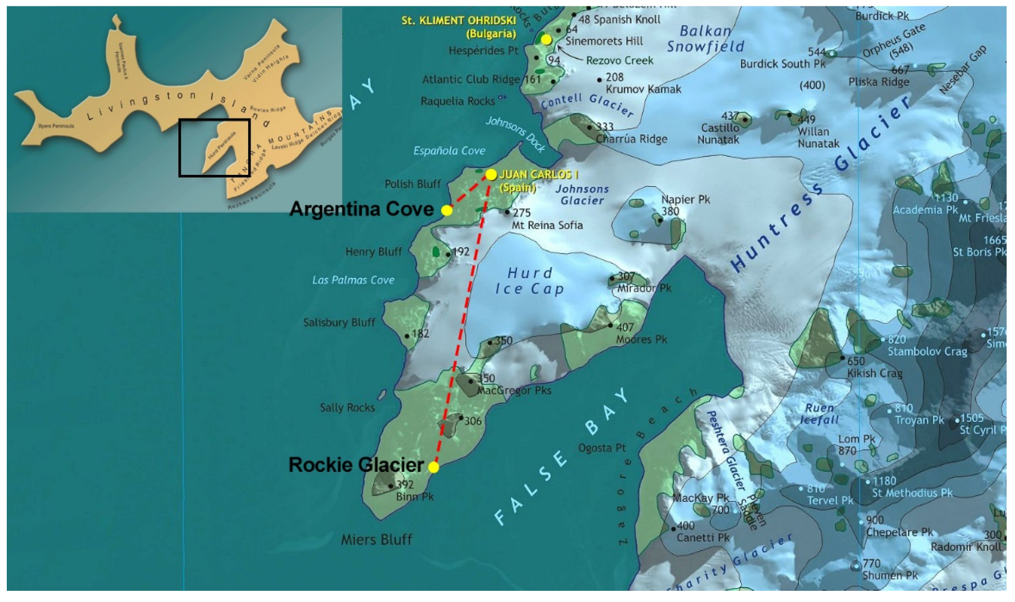
To achieve the proposed goal, our research group installed a sounding system [28] during the Spanish Antarctic Campaign 2018–2019 between two points around the Spanish Antarctic Base Juan Carlos I: Argentina Cove (1.34 km away) and Rockie Glacier (5.7 km away), as shown in Figure 1. Our purpose was to have a near node with both groundwave and skywave propagation, and a distant node with only NVIS propagation.

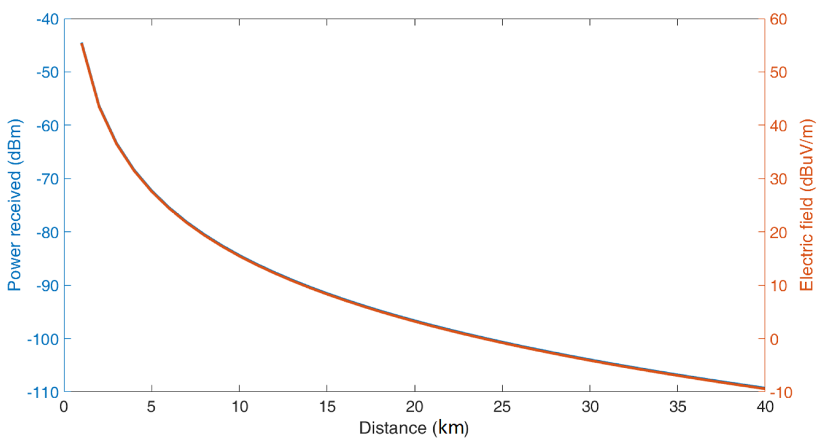
To decide the locations of each reception sounding system, the power reception of the groundwave have been studied depending on the distance. At Figure 2 we can see the groundwave electric field and power received depending on the distance from the Spanish Antarctic Base for a 24 W power transmission. As we can see, at Argentina Cove, the expected groundwave power received will be about −44.39 dBm, while at Rockie Glacier, it will be about −75.47 dBm. To avoid the reception of the groundwave at Rockie Glacier, the sensitivity of the sounding system has been set beyond −75.47 dBm.

The expected power and electric field have been calculated taking into account the ITU-R P.368 of groundwave propagation [29]. By the use of the software GRWAVE we simulated the received electric field from which we can calculate the antenna factor (1) assuming an antenna gain of −10 dB and a frequency of 4.3 MHz. Finally, we can calculate the voltage received at the antenna (2) and calculate the power received assuming 50 Ω.

$$\mathrm{K}\left(\mathrm{dB}/\mathrm{m}\right)=20\log \left(\mathrm{f}\right)-\mathrm{G}\left(\mathrm{dB}\right)-29.78$$

(1)

$$\mathrm{V}\left(\mathrm{dBuV}\right)=\mathrm{E}\left(\mathrm{dBuV}/\mathrm{m}\right)-\mathrm{K}\left(\mathrm{dB}/\mathrm{m}\right)$$

(2)

2.1. Overview of the System

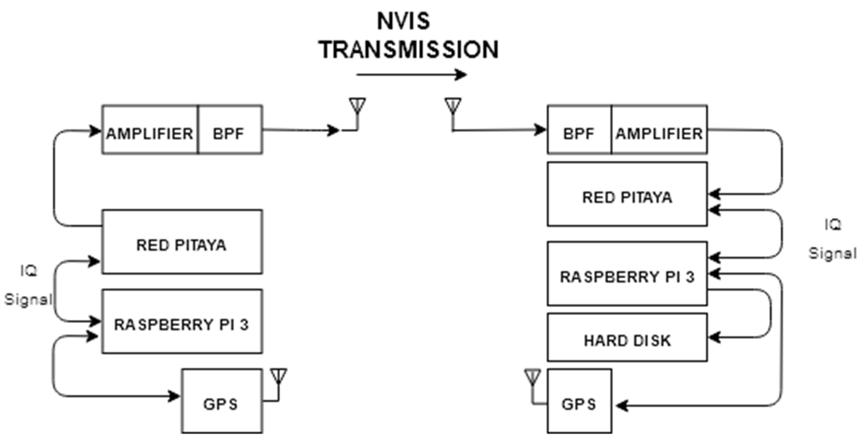
The block diagram of the sounding system can be seen in Figure 3. As it is a Software Defined Radio approach, you can select any carrier frequency, baseband data and bandwidth in a very easy way. The system is formed principally by a Red Pitaya platform [30] and a Raspberry Pi 3 with some peripherals.

The core of the system is the Red Pitaya platform which is in charge of the real-time processing signal tasks of up-converting and down-converting the data. The core of the Red Pitaya is a Zynq 7010 chip composed of an Advanced RISC Machine (ARM) processor and a field-programmable gate array (FPGA). Also, it is important to highlight that the board includes two analog-digital converter (ADC) and two digital-analog converter (DAC) of 14 bits and 125 MSPS. The internal structure of the programmed system on Red Pitaya is shown at [31].

The Raspberry Pi 3 is the microprocessor that controls all the peripherals. It is connected to Red Pitaya via ETHERNET and stores the received baseband in an external hard disk for further processing or sends to Red Pitaya the data which has to be transmitted. The output power of the amplifier can be selected from 1 W to 24 W. The system can also be programmed to transmit different patterns every minute, so you can perform a set of different tests every hour.

On the other hand, the GPS receiver is used to synchronize the transmitter and the receiver system to send and receive at the same time the NVIS transmission. The transmitter amplifier has 50 dB of gain and the Low Noise Amplifier (LNA) at the receiver has 30 dB of gain followed by a band pass filter (BPF) between 3 MHz and 7 MHz.

The NVIS antenna is an inverted-V as the best option as we can see at [13] with 2 dBi of gain. The carrier frequency was selected as a result of the analysis of the critical frequency of the F2 layer (foF2) of the previous months. The optimum transmission frequency is usually selected as the 85% of foF2 and it was finally set to 4.3 MHz. The inverted-V antenna was installed using a central mast 13 m high. This antenna has a similar behavior than the horizontal dipole, but it only needs one single mast, so it is much easier to deploy. On the other hand, the inverted-V has a higher vertical polarization component than the horizontal dipole. This is an important issue for the groundwave, which mainly propagates only the vertical component of the electric field.

Finally, for analyzing all the data, Matlab software [32] has been used for demodulating all the data received and perform all the post-processing analysis, as it will be explained in Section 3.1.

2.2. Frame Design

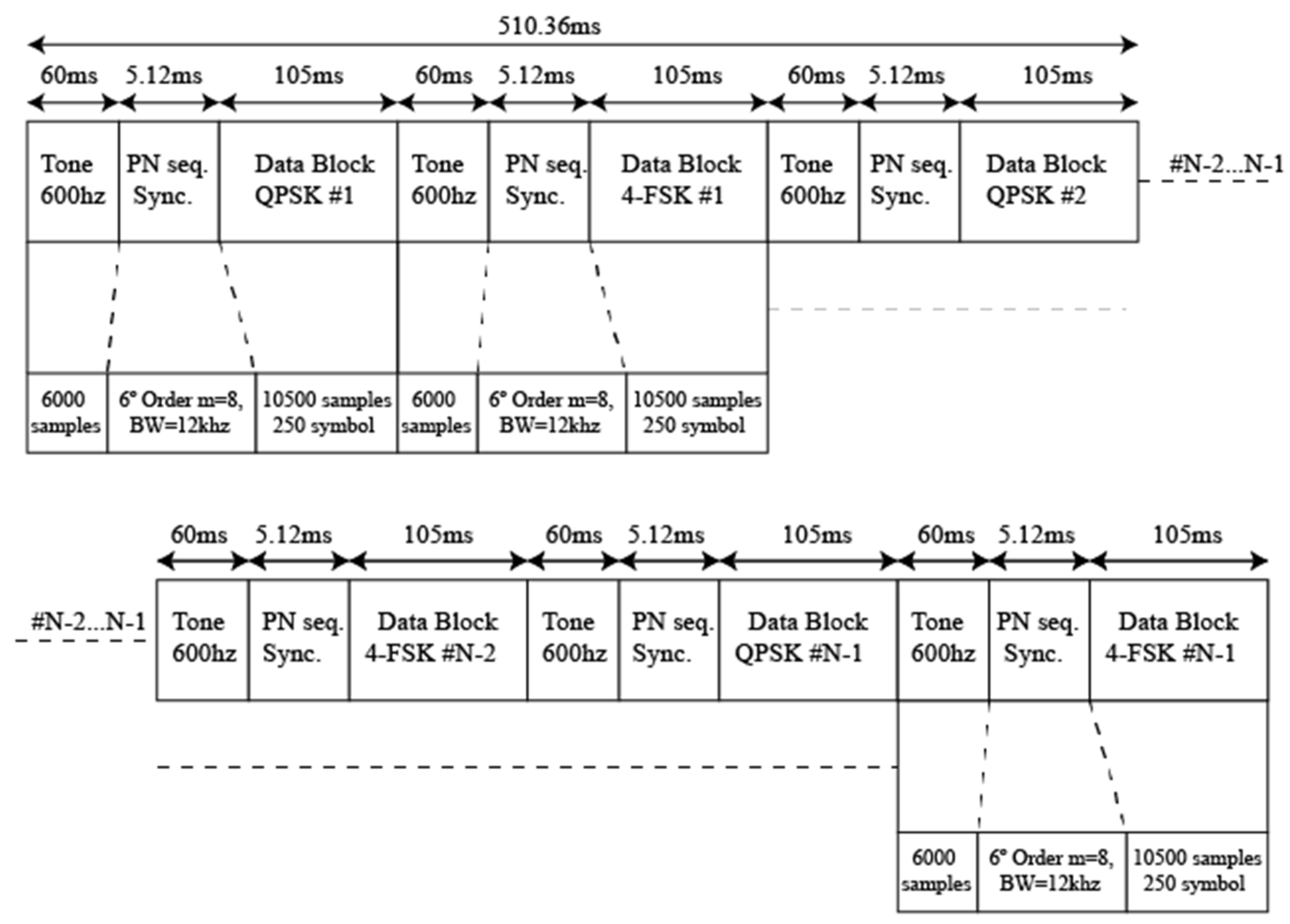
To measure the main channel characteristics, we transmit 150 packets made up of a 600 Hz tone, a 6th order PN sequence and a 250 symbols modulation of 4th order phase shift keying (PSK) and Frequency Shift Keying (FSK) as we can see in Figure 4. All the packets have to be carefully designed to be consistent with the Doppler spread and the delay spread of the channel. In particular, each 600 Hz tone has a time duration of 60 ms, the PN sequence a duration of 5 ms and the modulation a duration of 105 ms. All 150 packets in the transmitted frame have a duration of 25.5 s. To estimate the effects of the channel on the modulations, we transmit a different 4th order modulation in each packet. 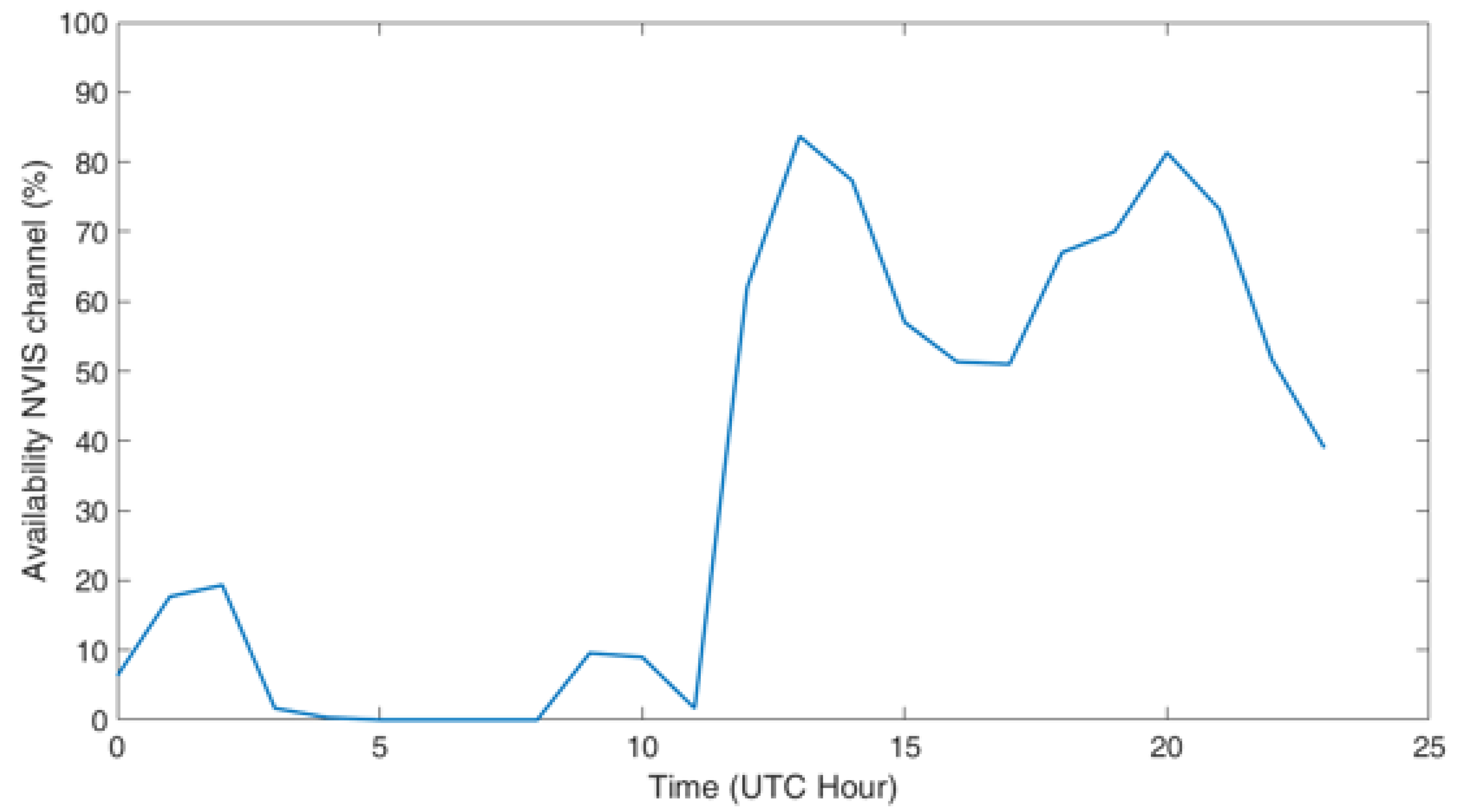The two packets have a total duration of 340 ms, which is less than the expected coherence time of the channel [23]. The tests were performed 24 h a day every 10 min between the 10 and 22 of February of 2019.

First of all, the 600 Hz tone is used for analyzing and correcting the Doppler shift effect on the received frame. This frequency shift is not mainly produced by the ionosphere, but it is caused by the low stability of the clocks of the Red Pitaya platform. This makes the estimation of the ionosphere Doppler shift effect not possible. The use of a 600 Hz tone for correcting the Doppler shift instead of a DC constant is because with a 600 Hz tone the measure of the Doppler shift frequency can be done with a shorter packet. In this case, the Doppler shift effect will variate the 600 Hz tone between 580 Hz and 620 Hz. For assuring the measure of the Doppler shift, we estimate that the Doppler shift can be in the worst case of 50 Hz. In this case estimating the frequency of 550 Hz tone, the measure could be done with 33 cycles (60 ms). The case of using a DC tone, for measuring 1 Hz of Doppler shift, the measure would consider only a 16th part of a cycle (60 ms), which is not enough for an accurate result.

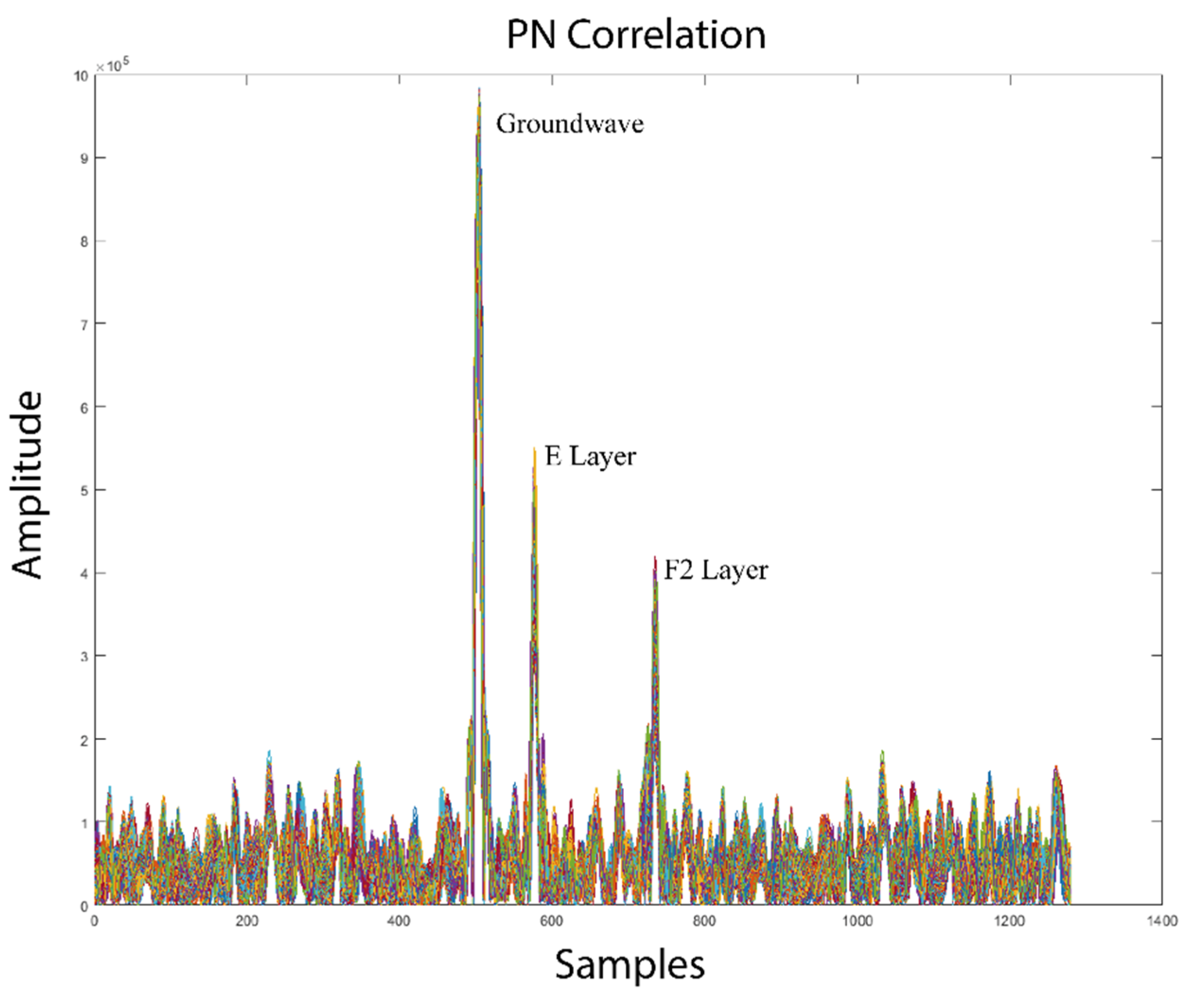
Then, a PN sequence is used for both estimating the channel response in terms of delay spread and Doppler spread and time synchronization. It is a 6th order PN sequence with a resampling of 8 that has been carefully designed in order not to be affected by the delay spread, the Doppler spread and Doppler shift. The nodes located at Rockie Glacier and Argentina Cove will receive the frame and correlate the received sequence with a local replica, so the output is an estimation of the channel response as a function of time.

Finally, the data blocks allow us to study the robustness of 4th order modulations under the NVIS channel. The test has been done with two different modulations: QPSK and 4FSK. The modulation QPSK shares the same features as the standards STANAG and MIL-STD 188 110C Appendix D in terms of bandwidth and bitrate. In this case, the QPSK has been equalized with a decision feedback equalizer (DFE) with a recursive least squares (RLS) algorithm to mitigate the effects of the intersymbolic interference (ISI). The ISI produced is caused by multiples reflections on the ionosphere and the terrain or by the presence of multiple ionospheric layers. According to previous studies [14], we selected a transmission power of 24 W to analyze the robustness of low power transmissions.

3. NVIS Channel Analysis

As stated before, we performed two simultaneous tests between Argentina Cove and the Antarctic Base Juan Carlos I and between Rockie Glacier and the base. These two locations allow us to distinguish the groundwave from the skywave, since the two locations have a similar behavior in terms of ionospheric reflection.

3.1. Postprocessing Analysis

To analyze all the parameters required to design a new frame protocol based on the NVIS channel we postprocess the received signal frame of Figure 4 in order to obtain key measured parameters. First of all, we obtain the Doppler shift by the 600 Hz tone and we locate the data block by the correlation of the PN sequences of all the frame. Once synchronized, we obtain the BER of each data block depending on its modulation. By the other way, the correlation of the PN sequence of one frame transmitted provides us a lot of information about the evolution of the skywave and groundwave channel impulse response. In Figure 5, we can see an example of a PN sequence correlation where we can see the received groundwave, the reflection at both the E layer and F2 layer.

The comparison between the correlation and the Livingston Island ionogram provided by Observatori de l′Ebre [33] provides us information about the origin of each path. As we can see in Figure 6, the ionogram shows us the height in the Y-axis for both the E layer and F2 layer for every frequency carrier transmitted in the X-axis. We can see that the E layer reflects a 4.3 MHz signal on a height of 120 km approximately and the F2 layer reflects a 4.3 MHz signal on a height of 310 km. If we analyze Figure 5 for the PN sequence correlation, we can note than the first peak is produced by the groundwave which is the first to be received. The second peak is produced by the ionospheric reflection of the E layer, received 800 microseconds later, equivalent to 240 km approximately. A half of this distance match with the height of the E layer as we can see on the ionogram. The third peak is produced by the ionospheric reflection of the F2 layer, received 2066 microseconds later, equivalent to 620 km approximately. Half of this distance match with the height of the F2 layer as we can see on the ionogram. Furthermore, a multipath of 33 microseconds is produced by the ordinary and extraordinary waves at the F2 layer with an effect produced on the received frame.

From the PN sequence correlation of Figure 5, we can obtain the delay spread (σ_τ) as the r.m.s. delay value of the signal as a density function S(τ):

$$\overline{\mathsf{\tau }}={{\displaystyle \int }}_{-\infty }^{+\infty }\mathsf{\tau }\mathrm{S}\left(\mathsf{\tau }\right)\mathrm{d}\mathsf{\tau },$$

(3)

$$\overline{{\mathsf{\tau }}^2}={{\displaystyle \int }}_{-\infty }^{+\infty }{\mathsf{\tau }}^2\mathrm{S}\left(\mathsf{\tau }\right)\mathrm{d}\mathsf{\tau },$$

(4)

$$\mathsf{\sigma }\mathsf{\tau }=\sqrt{{{\displaystyle \int }}_{-\infty }^{+\infty }{(\mathsf{\tau }-\overline{\mathsf{\tau }})}^2}\mathrm{S}\left(\mathsf{\tau }\right)\mathrm{d}\mathsf{\tau }=\sqrt{\overline{{\mathsf{\tau }}^2}-{(\overline{\mathsf{\tau }})}^2},$$

(5)

where $\mathsf{\tau }$ is the time sample and $\mathrm{S}\left(\mathsf{\tau }\right)$ the amplitude. For better comprehension, the delay spread of the groundwave by the dispersion of the first peak. Moreover, the delay spread of the skywave is obtained using the distance in time from the second peak (E layer) and the last peak (F2 layer).

To obtain the scattering function $\mathrm{S}\left(\mathsf{\tau };\lambda \right)$ [27] of the skywave:

$$\mathrm{S}\left(\mathsf{\tau };\mathsf{\lambda }\right)={{\displaystyle \int }}_{-\infty }^{+\infty }\mathrm{Rc}\left(\mathsf{\tau };\mathsf{\Delta }\mathrm{t}\right){\mathrm{e}}^{-\mathrm{j}2\mathsf{\pi }\mathsf{\lambda }\mathsf{\Delta }\mathrm{t}}\mathrm{d}\mathsf{\Delta }\mathrm{t},$$

(6)

where $\mathrm{Rc}\left(\mathsf{\tau };\mathsf{\Delta }\mathrm{t}\right)$ gives the average power output as a function of the time delay $\mathsf{\tau }$ and the difference $\mathsf{\Delta }\mathrm{t}$ in observation time We make use of 150 PN sequences of a frame without the groundwave. From the scattering function, we can measure the Doppler spread of the skywave channel. We proceed in the same way for the calculation of the Doppler spread of the groundwave.

3.2. Results Obtained

In this section are the detailed results obtained in terms of availability of the NVIS channel, height of layers, delay spread, Doppler spread, and bit error rate (BER) for both groundwave and skywave channels.

First of all, we evaluate the availability of the two implemented nodes. In Figure 7 we can see the percentage of packets detected and demodulated at 4.3 MHz with the node of Rockie Glacier. It is important to analyze this graphic for knowing the impact of the received frames in other graphics based on the time. As we can see the best availability of the channel is between 12 UTC and 21 UTC when the solar activity is higher. We have to consider that, for that time of year, the sunrise is at 8 UTC and the sunset at 1 UTC in Livingston Island. Furthermore, between 15 UTC and 19 UTC there is a reduction of the received packets. This is produced as we can see in Figure 8 by the presence of two layers which increase the delay spread.

The solar activity is highly related to the height of the ionospheric layers during the day for a 4.3 MHz transmission. In Figure 8 we can see between 11 UTC and 23 UTC the emergence of the E layer due to the major solar activity, which coincides with the sunrise at 8 UTC and the sunset at 1 UTC of Livingston Island. As we can see in Figure 8, the height of the F2 layer is around 400 km during the hours of low solar incidence (between 0 UTC and 7 UTC), while it decreases to 275 km during the hours of high solar incidence. During the hours of the emergence of the E layer, the skywave will be reflected at two layers physically separated 250 km approximately, increasing the multipath and directly the BER of the demodulated data due to the ISI. The delay spread will be even higher in the presence of the groundwave. It is also important to denote that during the major solar activity, a layer situated below the E layer, the D layer will appear. In Figure 8, we can see that the F2 layer disappears, due to the attenuation of the PN sequence signal at the D layer [26] making weak the signal reflected at the F2 layer and not being detectable by our system.

Once analyzed the channel availability and height of the ionosphere layers for different hours, in Figure 9 we analyze the total delay spread of the NVIS channel received at Rockie Glacier for different hours (see Figure 9). The delay spread is a very important parameter to determine the ISI effect on the transmitted frame. For an NVIS channel the maximum delay spread is 2.75 ms, so if we consider 0.42 ms the time of a symbol transmitted according to the standards STANAG and MIL-STD-188 110, the symbols transmitted will present ISI effect. This maximum delay spread calculated corresponds to a coherence bandwidth of 363.64 Hz. We can also observe that the minimum delay spread is 0.05 ms. In this case, the delay spread is less than the symbol time transmitted so there will not be ISI effect. Even so, the mean delay spread is a bit more than the symbol time, so the ISI effect will be present for most of the transmissions. In this case, the minimum delay spread corresponds to a coherence bandwidth of 20 kHz.

In Figure 10, we can analyze the total delay spread of both the NVIS channel and the groundwave channel at different hours for the node located at Argentina Cove. This is a key issue for designing the frame protocol frame since the presence of the groundwave which becomes the shorter path. This new path changes the skywave to a multipath making the delay spread highest than Rockie Glacier. In this case we can observe the maximum delay spread presented during the day, which will define how the frame protocol has to be prepared to avoid ISI for both skywave and groundwave. As we can see the highest delay spread is 5.5 ms which is equal to a coherence bandwidth of 181.8 Hz. If we consider a time symbol of 0.42 ms as the standards STANAG and MIL-STD-188 110, we can observe that the received frame will present strong ISI among symbols. On the other hand, the minimum delay spread for the groundwave when the reflection by NVIS channel is not available is approximately 0.05 ms, which corresponds to a coherence bandwidth of 20 kHz.

The Doppler spread gives us information about the variability of the channel and it has to be analyzed when designing a new communications frame protocol. In Figure 11 we can analyze the Doppler spread of the NVIS channel received at Rockie Glacier without the groundwave. The figure shown is a boxplot for the different hours during the day where the red line is the mean Doppler spread received, the blue square the 50% of the Doppler spread received, the black line is the 25% upper and down Doppler spread received and the red crosses are outliers of the percentages. As we can see, the maximum Doppler spread of the channel is about 0.1 Hz (10 s) and the minimum near 0.05 Hz (20 s). This value is a key issue to determine the maximum time of the data block. Despite the measured value, the data block set will be the same as the HF standards to allow for an easier comparison.

On the other hand, we can analyze the Doppler spread of the groundwave in Figure 12. In this case, the maximum Doppler spread is about 0.088 Hz (11.36 s) and the minimum near 0.062 Hz (16.12 s), so the channel can be considered quasi-stationary since the variations are only caused by the changes of the dielectric constant of the earth. These variations at Livingston Island are produced by the terrain snow and ice changes [29]. Furthermore, the groundwave of Argentina Cove can be received by the sea instead of the signal crossing the mountain as we can see in Figure 1. The Doppler spread variations can be also produced by the daily changes of the sea surges.

In Figure 13 we can analyze the Doppler shift produced by the clocks of the Red Pitaya platform. The Doppler shift in this case is directly related to the temperature of the platform, which will affect the stability of the clock. The Doppler shift caused by the ionosphere will be negligible compared to the variation of the clocks, especially in low cost platforms. As we can see, the maximum Doppler shift received is −17.5 Hz and the minimum −12.5 Hz.

Finally, we can study the probability to receive a BER value under the skywave channel effects for both nodes. For that purpose, we will analyze the Cumulative Distribution Function (CDF) of the BER demodulated for the transmitted modulations of order 4 at 24 W and 2.3 kHz of bandwidth. The CDF shows us the probability of achieving a BER lower than a given value. In Figure 14, the Y-axis shows us the probability of receiving a BER less or equal than a value Xo of X-axis in Rockie Glacier. As we can see, the probability of receiving a BER lower than 2 × 10⁻³ is about 84.2% for the QPSK and a 57.2% for the 4FSK. As we can see the QPSK is most robust in front of the NVIS channel effects. It is important to note that the QPSK modulation has been equalized, while the 4FSK was demodulated without equalization. The 4FSK do not need an equalization because the phase shift does not affect the received frequency.

Finally, we can analyze in Figure 15 the CDF of both groundwave and skywave received data at Argentina Cove. In this case, as we have seen, the delay spread is higher than the skywave delay spread received at Rockie Glacier. As we can see, the probability to achieve a BER lower than 2 × 10⁻³ is about 81.1% for the QPSK and a 53.8% for the 4FSK. Despite the fact that the received data present a delay spread higher than the skywave channel, the ISI effect is the same. This is why the results are similar to the skywave results.

To conclude this section, we can summarize all the results measured in

Table 1. Measured NVIS channel parameters.

Parameter	Skywave		Skywave + Groundwave
	Maximum	Minimum	Maximum	Minimum
Availability (12 UTC to 00 UTC)	84%	51%	100%	100%
Delay Spread	2.75 ms	0.05 ms	5.5 ms	0.05 ms
Doppler Spread	0.1 Hz	0.088 Hz	0.05 Hz	0.062 Hz
Doppler Shift	−17.5 Hz	−12.5 Hz	−17.5 Hz	−12.5 Hz
	QPSK	4FSK	QPSK	4FSK
Probability for BER < 2 × 10−4	84.2%	57.2%	81.1%	53.8%

.

4. Frame Protocol Definition

As we analyzed in the previous chapter, there are several parameters to consider for the definition of the signal frame according to the channel requirements depending on the distances to communicate. The current HF Frame Protocol Standards MIL-STD 188 110C Appendix D and STANAG are designed for both oblique and NVIS transmissions without considering the possibility of receiving the groundwave. These facts make not at all the most efficient way for short range NVIS transmissions, moreover with groundwave presence. As we have seen, the delay spread is a very important parameter to take into account, with very different values between an NVIS channel and an NVIS channel with groundwave presence. For that reason, it is advisable to design a signal frame different for each situation. The current standards make use of narrowband modulations for the transmission of data. These modulations are especially affected by the delay spread producing ISI on several contiguous transmitted symbols. The correction of this type of channel effect is hardware expensive to achieve low BER values. The equalization of narrowband modulations in time domain needs a long frame header of known symbols that decrease the efficiency of the frame, especially for high delay spread values.

To assure the correct transmission, we can make use of different techniques to avoid the different effects produced by the channel. First of all, spread spectrum (SS) techniques can be applied to increase the bandwidth of the signal. The use of these methods can make more secure and increase the robustness in front of interferences and noise. However, in this study, we want to maintain the HF standards signal bandwidth. For that purpose, we propose the use of OFDM modulation to ensure a robust communication without equalization in time domain to avoid ISI. The OFDM modulation is based on dividing a wideband modulation on several narrowband modulations. This makes each narrowband modulation to have a flat fading channel even if the channel is frequency selective, avoiding the use of complex equalizations. In our proposal, we use a simple and low cost Zero-Forcing equalizer instead of the standard decision feedback equalizer (DFE). Moreover, we can find different OFDM variations as single carrier-frequency division multiple access (SC-FDMA) or orthogonal frequency division multiple access (OFDMA). These OFDM variations are designed to assign different OFDM subcarriers to users as multiple access techniques. In addition, these variations have some advantages as a low Peak to Average Power Ratio (PAPR). In this study, the communication is based without differentiation of users and we wanted to base our design in the basis of the OFDM modulation to show the advantages of the cyclic prefix in front of the ISI as an alternative to narrowband modulations used on the HF Frame Protocol Standards. Even so, the modulation to be used will be a single carrier-frequency domain equalization (SC-FDE) as it is proposed at [34] by the addition of a DFT on the symbols to be transmitted and an IDFT after demodulating the symbols at reception.

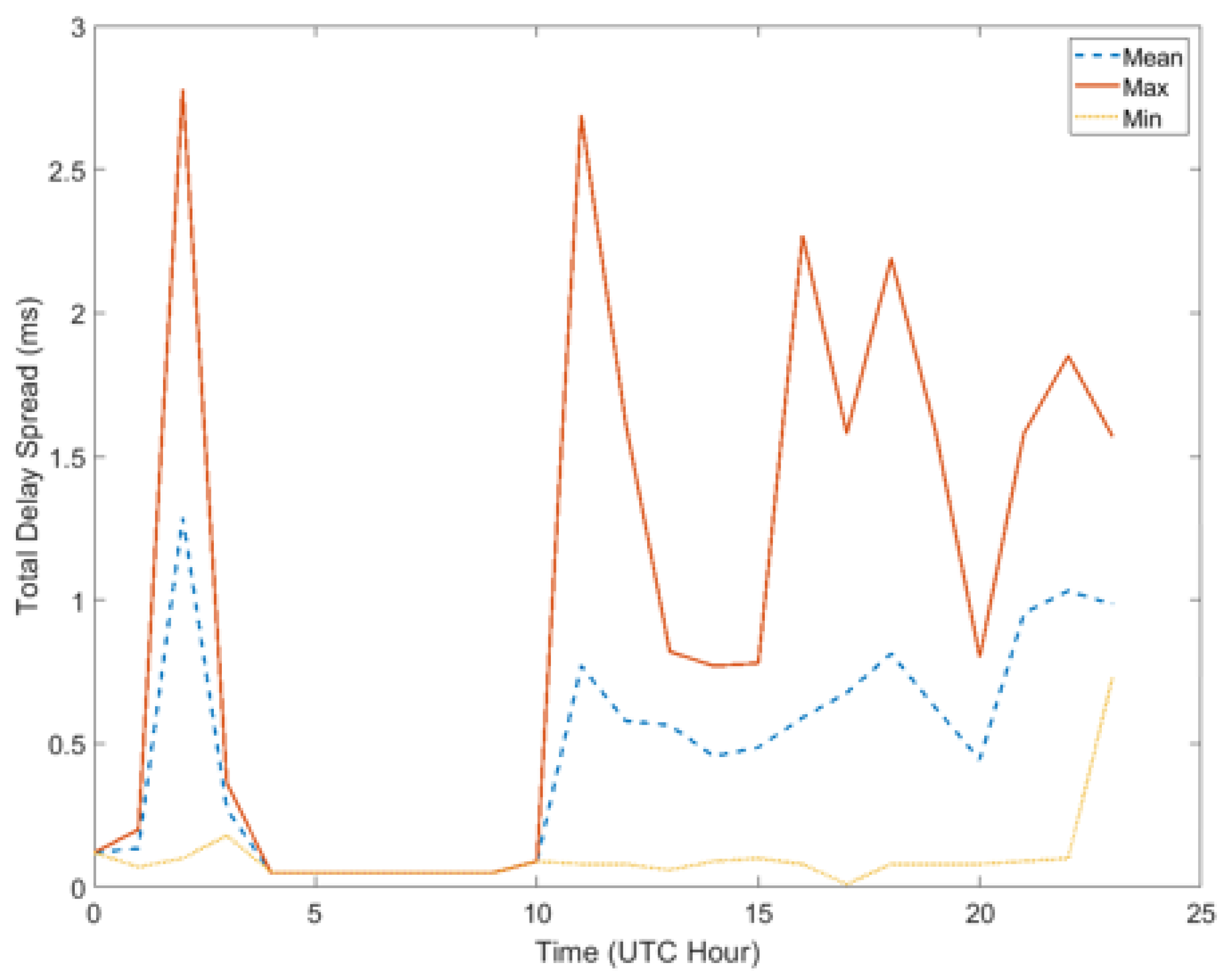
For the frame protocol design, there are two different scenarios, depending on the presence of the groundwave we propose two different cyclic prefix values to cancel the ISI [35]. In the case of an NVIS without groundwave communication, first of all, we took into account the maximum delay spread measured in Figure 9. This is the key parameter while designing the OFDM to avoid the ISI effects produced by multipath. For this configuration, we set the cyclic prefix to 2.75 ms leaving a margin of 0.25 ms to ensure the correct use of it. The duration of the useful symbol length is a key issue because it determines the number of subcarriers that will be allocated in a 3 kHz band. For a low power transmission, we cannot have too many multiples subcarriers because the energy per bit to the spectral noise (E_b/N₀) received of a single subcarrier will be very low. Moreover, the number of subcarriers has to be consistent with the number of equalization pilots to be positioned in the most efficient way. On the other hand, the minimum number of subcarriers is set to achieve the bitrate requirements. It is also important to obtain an OFDM symbol time nearly multiple to the time data block of the standards at 3 kHz of bandwidth. Bearing all that in mind, we set the useful symbol length to 9.33 ms to configure the OFDM with 28 subcarriers, 7 OFDM symbols and a total data block time of 86.31 ms. To allow a better comparison, the number of OFDM symbols has been set to obtain the most similar data block time with the HF data transmission frames. In addition, the minimum measured coherence time of the channel is 10 s, as we can see both frame structures accomplish the coherence time. According to the accomplishment of the coherence time measured in all the data block, only one OFDM symbol will be set as pilots to estimate the frequency variations. In the other side, the bandwidth of each subcarrier is about 107 Hz to assure the accomplishment of the 363.64 Hz coherence bandwidth of the measured channel and a total of 27 subcarriers will be used as data subcarriers. Finally, as shown in Figure 14, we tested the robustness between the QPSK and the 4FSK, and the results showed the QPSK as the best modulation for the data subcarriers of the OFDM. Also, we can contrast our results [14], where the QPSK shows to be a robust option for low power transmissions. Taking into account the DC null and the equalization pilots, the useful bitrate of the OFDM configuration is about 1.741 Kbps. In

Table 2. OFDM configuration for NVIS transmission.

Bandwidth	3 kHz
Useful symbol length	TS = 9.33 ms
Prefix cyclic length	TCP = 3 ms
Number of subcarriers	NSC = 28
Number of symbols OFDM	NSOFDM = 7
Number of pilot OFDM symbols	NSP = 1
Number of data OFDM symbols	NSD = 6
Number of subcarriers DC NULL	NDC = 1
Time duration of OFDM packet	NPT = 86.31 ms
Bits in packet	Bits = 324 bits
Modulation	QPSK
Equalization	Zero forcing
Bitrate of signal frame	2.139 Kbps

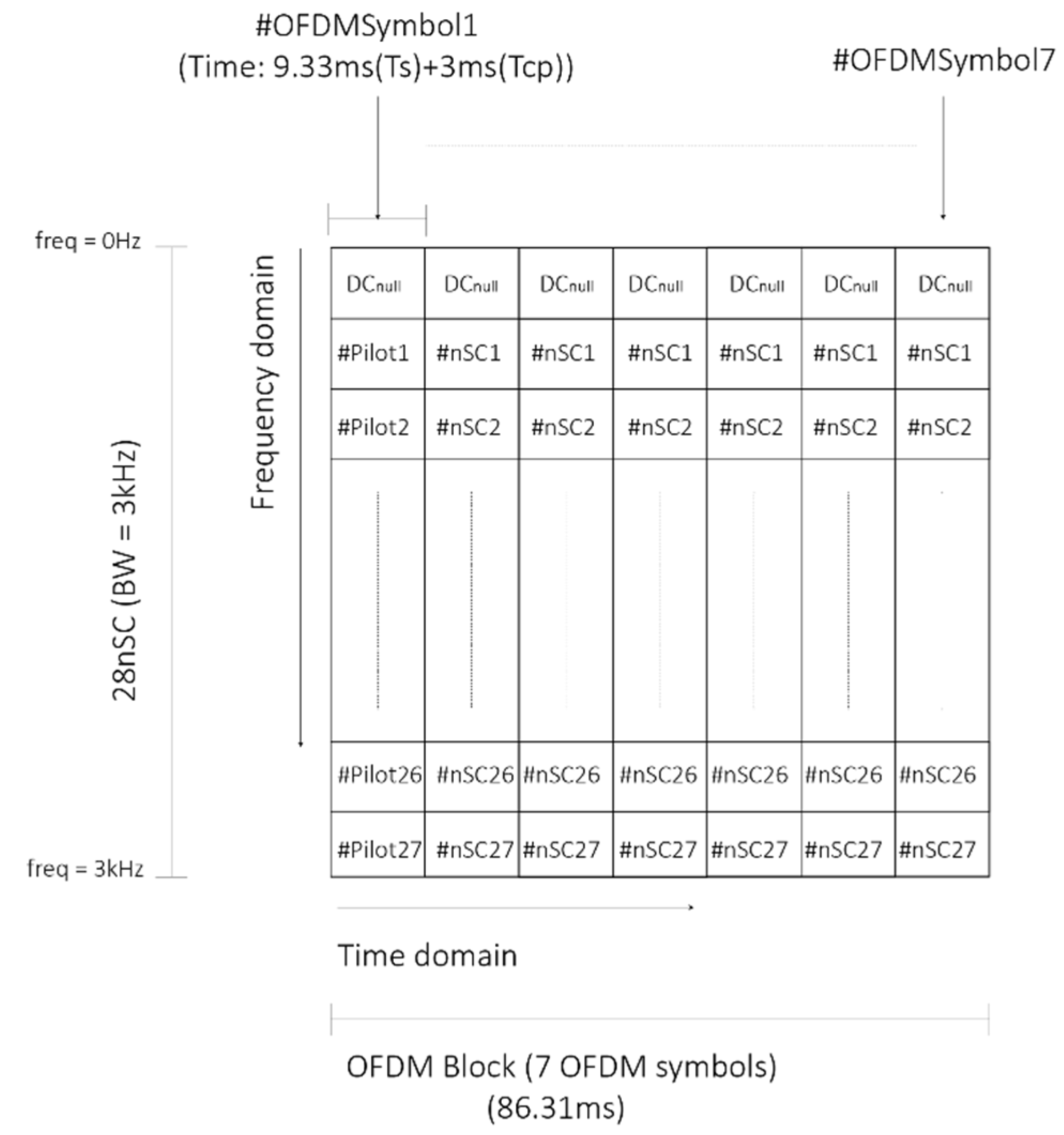
is summarized the OFDM configuration for an NVIS communication without groundwave. For a better comprehension of the designed data block, in Figure 16, we can observe the OFDM matrix in a time and frequency domain.

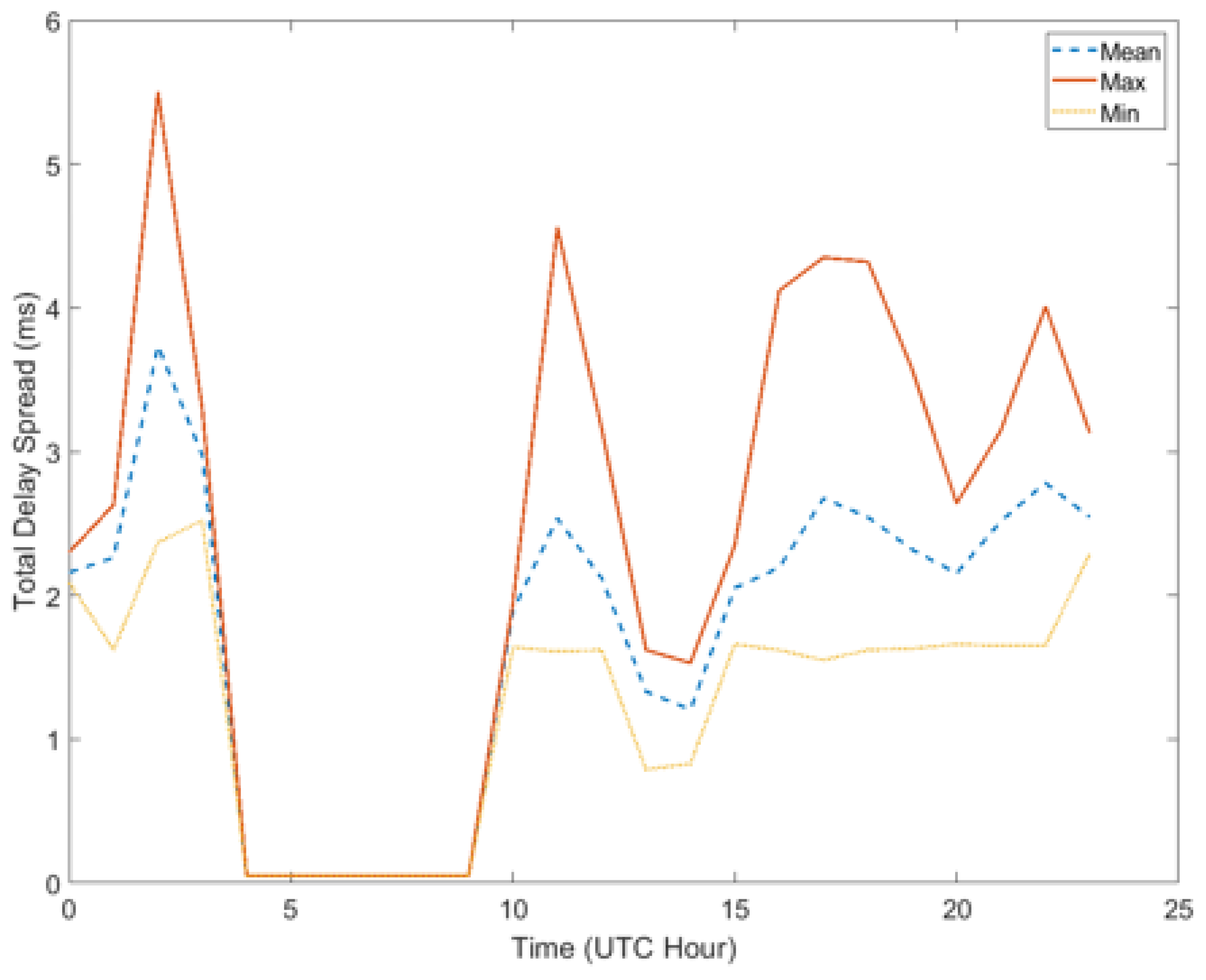
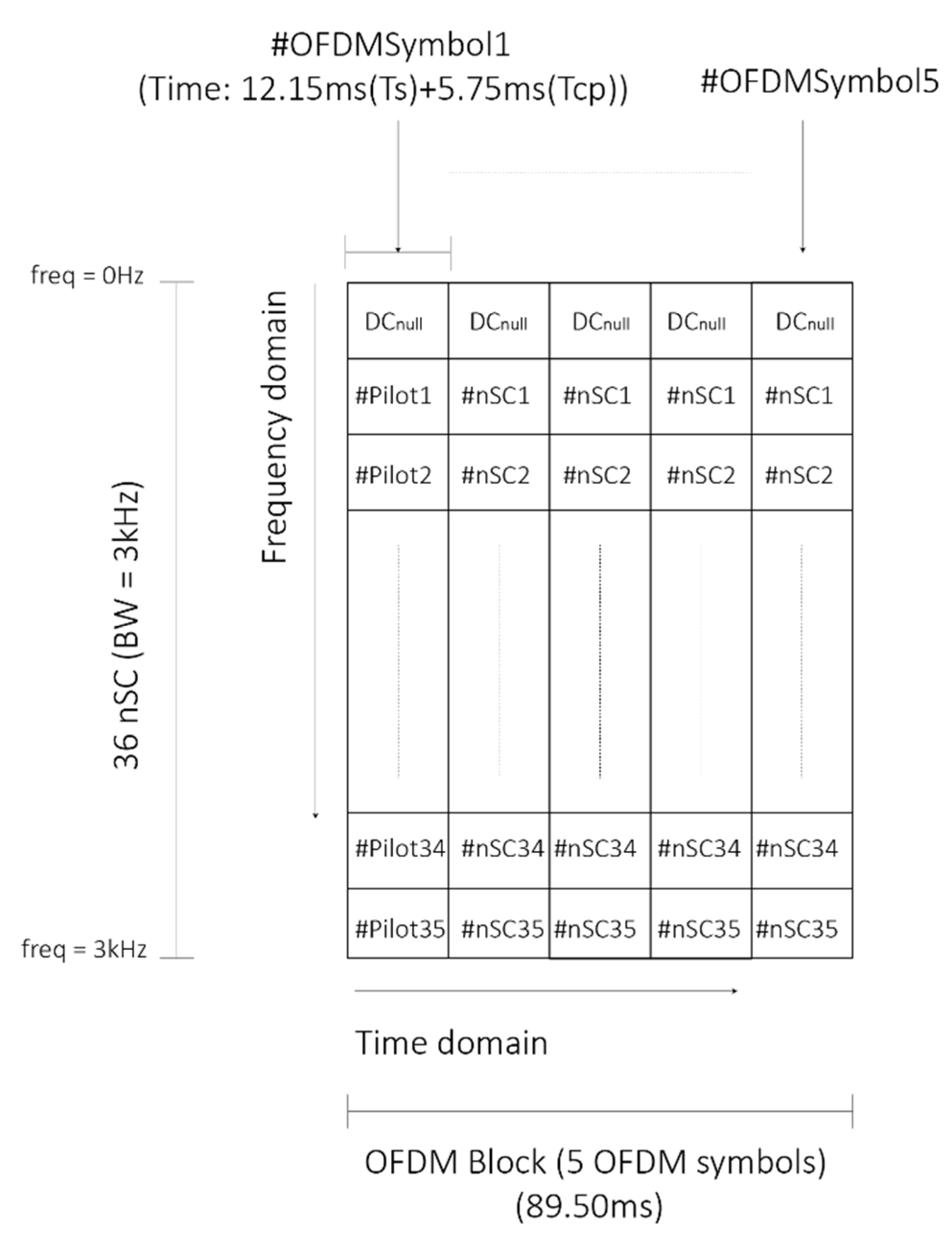
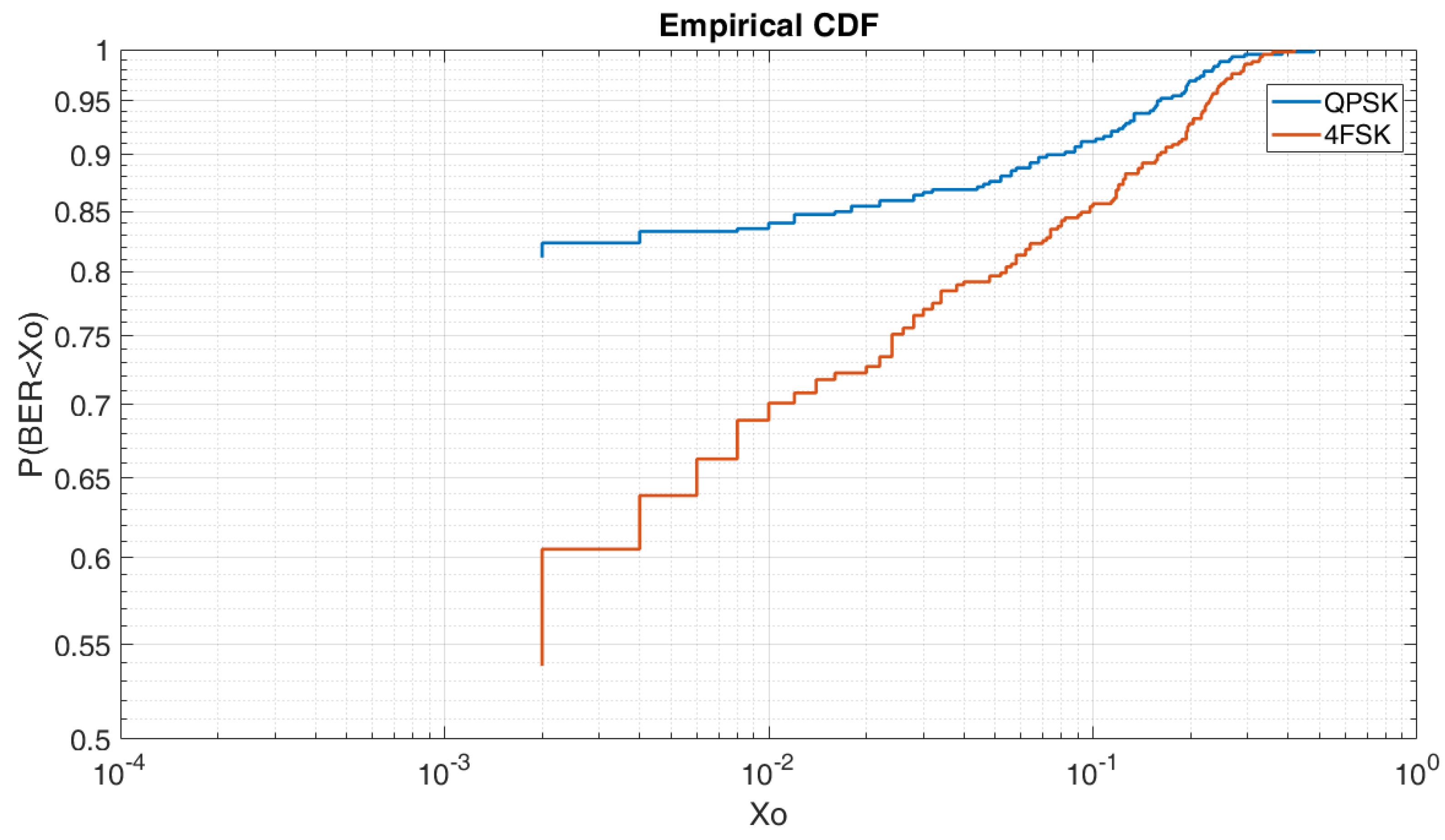
In the case of an NVIS with groundwave communication, as the previous configuration, we took into account the maximum delay spread measured in Figure 10 to avoid the ISI effects produced by the multipath. First of all, we configured the cyclic prefix to 5.75 ms leaving a margin of 0.25 ms to ensure the correct use of it. To maintain a similar block data time with the HF Frame Protocol Standards, we set the useful symbol length to 12.15 ms to configure the OFDM with 36 subcarriers, 5 OFDM symbols and a total data block time of 89.5 ms. According to the accomplishment of the coherence time measured in all the data blocks, only one OFDM symbol will be set as pilot to estimate the frequency variations. To be consistent with the coherence bandwidth measured of 181 Hz, the bandwidth of each subcarrier is set to 82.3 Hz increasing the number of subcarriers to 36. Finally, as we measured at Figure 15, the QPSK modulation is more robust in front of the 4FSK for this scenario. As the previous OFDM configuration, we modulate the data subcarriers with a QPSK due to its robustness for low power transmissions. Taking into account the DC null and the pilots to equalize, the useful bitrate of the OFDM configuration is about 1.130 Kbps. The bitrate for this configuration has decreased because of the increase of the cyclic prefix, the useful symbol length and the number of pilots. In

Table 3. OFDM configuration for NVIS with groundwave transmission.

Bandwidth	3 kHz
Useful symbol length	TS = 12.15 ms
Prefix cyclic length	TCP = 5.75 ms
Number of subcarriers	NSC = 36
Number of symbols OFDM	NSOFDM = 5
Number of pilot OFDM symbols	NSP = 1
Number of data OFDM symbols	NSD = 4
Number of subcarriers DC NULL	NDC = 1
Time duration of OFDM packet	NPT = 89.5 ms
Bits in packet	Bits = 280 bits
Equalization	Zero forcing
Modulation	QPSK
Bitrate of signal frame	1.810 Kbps

, the configuration is summarized to avoid the delay spread in an NVIS with groundwave communication. For a better comprehension of the designed data block, in Figure 17, we can observe the OFDM matrix in a time and frequency domain.

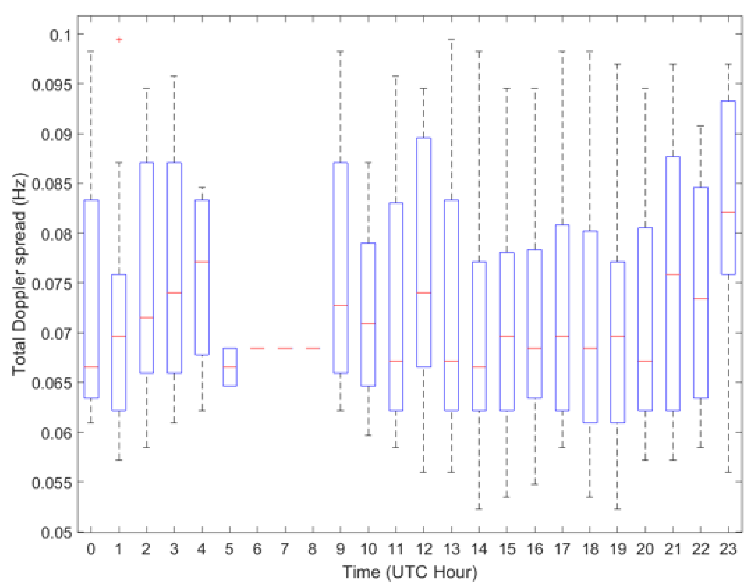
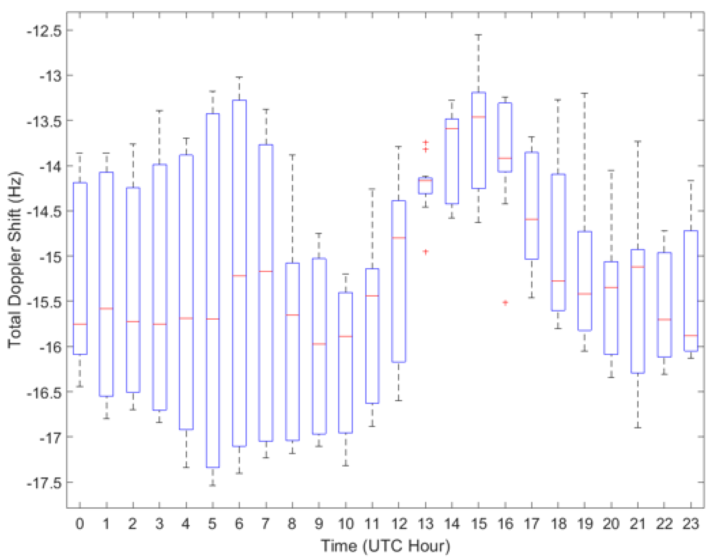
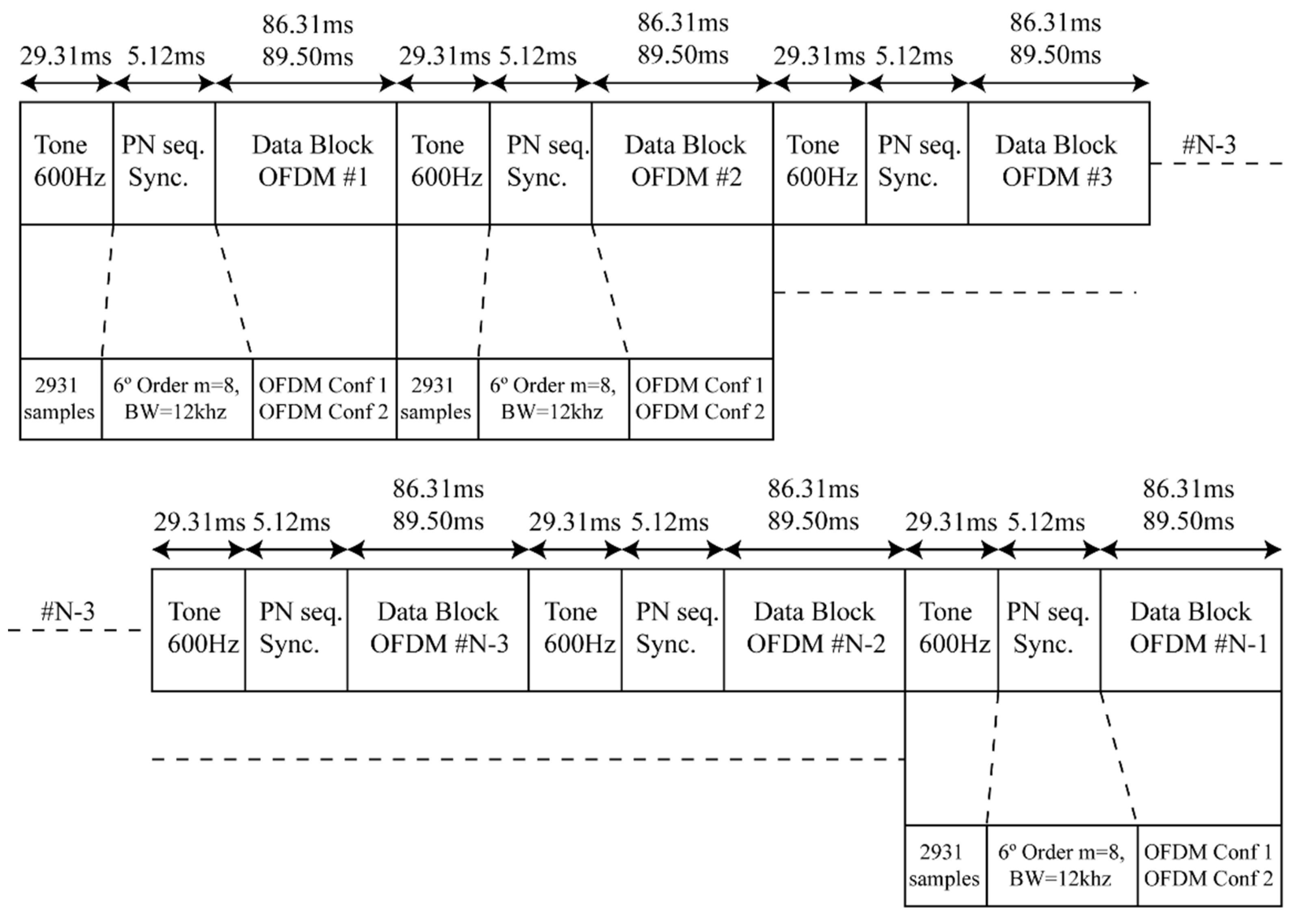
Once the OFDM data block of the new frame protocol is designed, it is important to take into account some preamble to avoid effects as Doppler shift and time synchronization. The preamble time required in the HF standards frames is about 34.33 ms. For a better comparison, we will take the same preamble time. First of all, the measured critical Doppler shift of Figure 13 is about −17.5 Hz. To avoid critical problems of frequency offset on the reception of the frame protocol and with the OFDM subcarriers, we will consider −20 Hz and we will introduce a 600 Hz tone at the preamble of all data blocks to measure the Doppler shift as we mentioned at Section 2.2. Taking 2.5 Hz of margin, in the worst case, we will receive a 580 Hz tone which can be correctly measured with 17 cycles being a total time of 29.31 ms. The estimation of the frequency offset can be corrected with an error of 0.01 Hz, being enough to assure the correct reception and demodulation of the OFDM subcarriers. Furthermore, to assure the time synchronization of the system with the data blocks received, the preamble will include 5.12 ms of a 6th order PN sequence with a resampling of 8 in order to not be affected by the delay spread, the Doppler spread and Doppler shift. Furthermore, every OFDM symbol takes 12.33 ms and 17.9 ms, with 1233 samples and 1790 samples respectively, which is enough to avoid time synchronization errors. Finally, it is important to take into account for the amplifier used to transmit the frame, the PAPR produced at the OFDM modulation. To avoid the PAPR, we can apply different techniques, such as clipping, coding, partial transmit sequence (PTS), and selected mapping (SLM). We have chosen the clipping technique, with a controlled input back-off (IBO) as it is the less complex method. The IBO is defined as the difference between the squared clipped power and the signal mean power without generating a non-linear distortion as we can see at [35]. In Figure 18, we can observe the designed frame protocol for USN NVIS systems. The OFDM data block can be adapted depending on the communication scenario.

5. Frame Protocol Defined and HF Frame Protocol Standards

Once designed, the new frame protocol taking into account most of the measurements done for an NVIS channel, we can compare the designed frame protocol with related works and the HF Frame Protocol Standards STANAG and MIL-STD-188-110D.

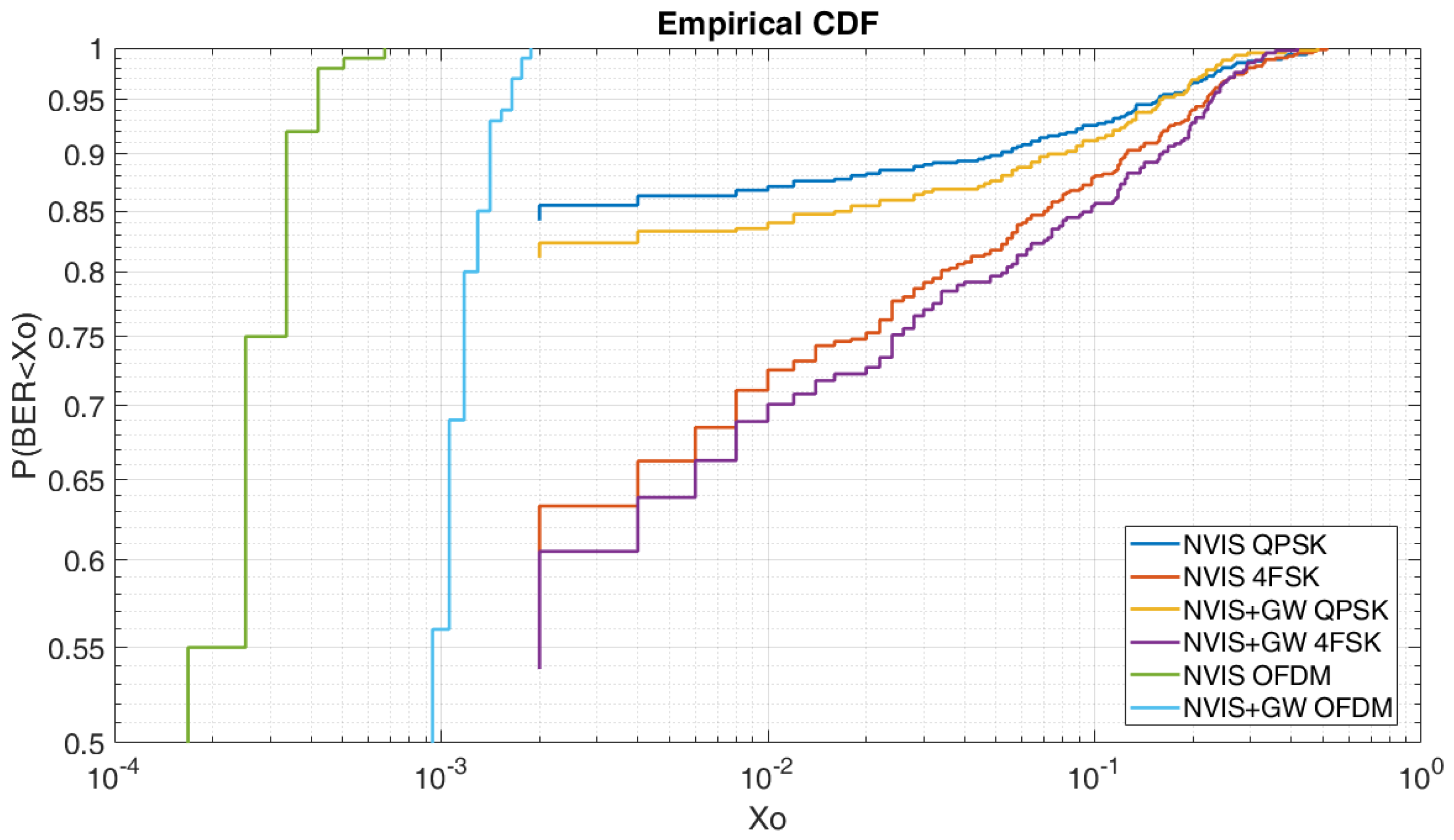
To evaluate the improvement, we run some simulations of our proposed frame protocol to compare it with real measured frame protocols based on the HF Frame Protocol Standards. The main focus of this comparison is the performance of the data block in front of the NVIS channel effects by the use of the preambles and modulation proposed. The NVIS channel simulation used for both multicarrier modulations is based on a Watterson channel model [36], which is obtained by adding two independent Rayleigh channels, each one with a frequency-shifted Gaussian Doppler spectrum to simulate the ordinary and extraordinary received waves as a bi-Gaussian Doppler spectrum. In Figure 19 we can see the results for both scenario cases of OFDM configurations in comparison with the real tested modulations used on the HF Frame Protocol Standards. Both OFDM simulations has been done with a total amount of 12 Mb. The channel simulation for the OFDM configuration of Table 1 has been set with two Rayleigh distributions, with a delay spread of 2.75 ms, an SNR of 6 dB and a Doppler shift of −17.5 Hz. The result shows us 84% of probability to receive a packet with a BER less than 3 × 10⁻⁴ in comparison of a BER less than 2 × 10⁻³ for the 4PSK and a BER less than 6 × 10⁻² for the 4FSK. The channel simulation for the OFDM configuration of Table 2 has been set with two Rayleigh distributions, with a delay spread of 5.5 ms, an SNR of 6 dB and a Doppler shift of −17.5 Hz. The result shows us an 81% of probability to receive a packet with a BER less than 10⁻³ in comparison of a BER less than 2 × 10⁻³ for the 4PSK and a BER less than 6 × 10⁻² for the 4FSK. As we can see, referring the simulation, we can realize that the new frame protocol configuration is more robust in front of the channel effects than the QPSK and 4FSK of Figure 14 and Figure 15 used on the HF standards. As we can see, the OFDM configuration of Table 2 is less robust than the OFDM of Table 1 because, for the same probability, it has a lower BER.

If we compare the obtained results with related works, Erhel at [20] study polarization techniques based on MIMO to make increase robustness and the bitrate of ionospheric communications. Even so, the use of polarization techniques requires two antennas for the transmission and reception and still not avoid the ISI effects in contrast to the frame protocol designed. Despite this, according to Erhel [20], MIMO polarization techniques can increase the bitrate of the HF Standards to 8.52 Kbps in the best channel conditions without ISI effect in comparison of 2.139 Kbps and 1.81 Kbps of the frame protocol designed for skywave and groundwave respectively. Despite this, in the case of high ISI effects produced by the presence of groundwave or by the NVIS channel, polarization techniques will not have any effect, it being impossible to establish the communication. In the case of using the frame protocol designed in this article, the ISI effect will be avoided. To improve the communication, MIMO techniques can be used on the frame protocol designed, assuring the communication with a bitrate of 4.28 Kbps and 3.62 Kbps respectively for skywave and groundwave. By the other way, Bergada at [22] studied OFDM and direct sequence spread spectrum (DSSS) transmission techniques for an HF communication of 12,700 km and it compares with the HF Standards for a slow fading multipath long-haul HF channel. For similar OFDM configurations (T_S = 10 ms, N_SC = 32, BW = 3.2 kHz, Modulation = QPSK, Bitrate = 4.102 Kbps) is achieved 50% probabilities to obtain a BER lower than 0.46 in comparison of both skywave and groundwave frame protocols designed where we have 50% probabilities to obtain a BER lower than 10⁻⁴ and 10⁻³ as we can see at Figure 19.

In addition to the comparison of Figure 19, in

Table 4. Main frame protocol differences.

Parameter	HF Standards	OFDM Skywave	OFDM Skywave + Groundwave
Preamble time	34.33 ms	34.43 ms	34.43 ms
Data block time	85.33 ms	86.31 ms	89.5 ms
Modulation	QPSK	OFDM QPSK	OFDM QPSK
Bitrate	4.26 Kbps	2.139 Kbps	1.81 Kbps
ISI effect robustness	No	Yes, from 10 km	Yes, from 0 km

, we compare the main characteristics of the frame protocol designed with the HF Frames Standards STANAG and MIL-STD−188-110D. As we can see, the preamble total time and data block time designed is very similar to the HF standards frames preamble and data block time. Nonetheless, the bitrate is lower for the designed frame protocol because of the modulations used for each frame protocol. Despite the low bitrate, it remains enough for most USNs and the use of this frame structure improves the robustness to ensure the data link.

6. Conclusions

In this article, we present a robust frame protocol for NVIS USN communications that performs better than the standards STANAG and MIL-STD-188-110D for distances between 0 and 250 km. To achieve these conclusions, we have taken measurement of an NVIS channel in two different scenarios: a single NVIS communication and an NVIS communication with the presence of groundwave. First, we analyzed the most critical values of the delay spread and Doppler spread scenarios. Then, we tested the robustness of QPSK and 4FSK in terms of BER. Finally, we measured the Doppler shift caused by the use of low stability clocks on a low-cost system.

Thereafter, we designed the NVIS signal frame protocol based on an OFDM. The use of an OFDM has two benefits: first, it is more robust in front of multipath signals due to the addition of a cyclic prefix. Second, the equalization in the frequency domain is much simpler. Also, the absence of ISI and the use of pilot subcarriers in the OFDM make the equalization of the signal easier. The simulations show a great improvement in comparison to the QPSK and 4FSK modulations for both NVIS channel scenarios.

The main drawback is that the use of an OFDM on the signal frame protocol decreases the bitrate in comparison to the standards STANAG and MIL-STD-188-110D. This is not critical for most USN requirements, especially for low bit rate remote sensors that do not have any other way to communicate.