Epidemic Source Detection over Dynamic Networks

Abstract

Epidemic source detection is one of the most crucial problems in statistical inference. For example, currently, the debate continues to reveal when and where the first spread of COVID-19 occured. For this problem, most of the works have assumed a static network topology, that is, the connections between nodes do not change over time. This is impractical because many nodes have some mobility in the network, or the connections can be changed. In this paper, we focus on the dynamic network, in the sense that the node connectivity varies over time. We first introduce a simple dynamic model, named k-flip dynamic such that $k>0$ connections in the network may be changed with some probability at each time. Next, we design a proper estimation algorithm using some investigation for the contact information between infected nodes, named dynamic network source estimation (DNSE)(k) for the dynamic model. We perform various simulations for the algorithm compared to several existing source estimation methods. Our results show that the proposed algorithm outperforms and is efficient for finding the epidemic source compared to other methods. Further, we see that the detection probability for our proposed algorithm can be above 45% when we use budget to investigate the contact information from the infected nodes under some practical setting of k.

1. Introduction

Epidemic diffusion processes in complex networks are ubiquitous in natural and technological systems. Examples include disease or epidemic spreading in the human society, virus invasion in computer and mobile phone networks, behavior propagation in online social networks [1]. Epidemic source detection is the problem that identifies the initial seed node of the diffused information (We use the terms “information” and “epidemic” interchangeably through the paper.) in the network. This is clearly of practical importance, because harmful diffusion can be mitigated or even blocked, e.g., by vaccinating humans or installing security updates. In the prior work, Shah and Zaman [2] showed that in the regular tree topologies, the detection probability cannot be above 31% under the Maximum Likelihood Estimator (MLE), and even worse, in other realistic topologies such as Facebook graphs, scale-free graphs and Internet Autonomous System (AS) graphs, the detection probability is less than 5% under a MLE-based heuristic due to a complex structure of networks. After this, extensive research attention for this problem has been focused on various network topologies and diffusion models [2,3,4,5,6,7,8,9], whose major interests lie in constructing an efficient estimator and providing theoretical analysis of its detection performance. Prior works revealed that finding the information source turns out to be a challenging task unless sufficient side information is provided. There have been several research efforts that use multiple snapshots [7] or side information about a restricted suspect which set the true source belongs [8], thereby the detection performance is significantly improved. Another type of side information is the one obtained from querying, i.e., asking questions to a subset of infected nodes and gathering more hints about who would be the true information source [10,11]. However, most of the works have assumed the static network topology, that is the connections between nodes do not change over time. This is impractical because many nodes have some mobility in the network, or the connections can be changed over time [12]. For example, users frequently changed their social contacts via meetings, emails, phone, and several online software. Hence, in this paper, we focus on the dynamic network, where the connections between node pairs are changed over time as in Figure 1. In this case, the information source may lose a graphical centrality of the snapshot from the frequent changes of connections. Under this consideration, we design a proper estimator, which is reflected in the dynamics of connection changes. This is not an easy task because it is no longer possible to estimate the location of the source of information through a snapshot of diffusion were most estimators are designed using this fact in static networks. To overcome this, we use some investigation process to obtain the contact information between nodes which propagating the information. Different to existing work [13], which assumed the infected node has side information of exact parent node of the spreading (i.e., who gives the information) over the time varying network, in our work, we focus on only the contact information for the diffusion without knowing the exact parent (This is a more practical scenario than that of [13] because we may not have the information about who spread it to me under some probabilistic diffusion process).

Our main contributions are summarized in what follows.

(1)

First, we consider a dynamic scenario for the source finding problem. To do that, we design a network dynamic model, named by k-flip dynamic, where the connectivity between node pair changes with some probability at each time among the k selected node pairs from the Erdös-Rényi (ER) random graph. This model covers various cases of changing the connections by varying the parameter $k.$ For example, a large k indicates a large portion of connections will changes, that captures more dynamical scenario of the connections whereas small k indicates a scenario where only a few changes occur in the network.

(2)

Second, we propose a source estimation algorithm. Based on frequent changes of connections in the network, we design the algorithm by two parts: (i) reconstruct contact graph and (ii) estimation of the source. In the first part, we rebuild the contact graph by some investigation process among selected nodes with the assumption that the investigator has budget $B>0.$ In the second part, we use a Short-Fat Tree (SFT) algorithm in [14] as a greedy estimator for the true source in reconstructed contact graph, which uses the node’s degree information for the ER random graph.

(3)

Third, we run various simulations using the proposed estimator. As comparison estimation algorithms, we use Jordan Center (JC) [5], Rumor Center (RC) [3], NETSLEUTH (NE) [15], Dynamic Importance (DI) [16] and Distance Center (DC) [2]. As a result, we see that our proposed method outperforms to others and the detection probability for our proposed algorithm can be above 45% when we use budgets to investigate the contact information between infected nodes under some practical setting of k whereas the fact that it is hard to beyond 50% even for static networks.

The remainder of this paper is organized as follows. Section 2 discusses related literature. In Section 3, we will introduce the network dynamic model, epidemic diffusion model, and investigation approach. Next, we propose a source estimation algorithm with its computational complexity. In Section 4, we depict the simulation results and some future works with a limitation of the paper, and we conclude the paper in Section 5.

2. Related Work

In this section, we summarize related studies by dividing them into the following two categories: (i) static networks, (ii) random and dynamic networks as describe in

Table 1. Taxonomy of epidemic source detection problems.

	Single Source	Multiple Sources
Static network	Rumor center [2,3,4], Jordan center [5,6], Multi-snapshots [7], Prior set [8], Decaying diffusion rate [9], Querying [10,11], Set estimator [17,18], Limit observation [19]	Minimum description length [20], Jordan Cover [21], Different diffusion time [22]
Random and dynamic network	Random growing graph [23], ER random network [14], Time varying network [13], this paper	Time varying network with sparse observation [1]

.

(i) Static Networks. As a first study with a static network, Shah et al. considered this problem [2,3,4] based on the rumor spreading over the network and introduced the metric called rumor centrality, a simple graphical metric for a given diffusion snapshot. They called a node that has maximum rumor centrality by rumor center the MLE. They proved that the rumor centrality implies the likelihood function when the underlying network is a regular tree, and the diffusion follows the Susceptible–Infected (SI) model, which is extended to a random graph network in [3]. Zhu et al. [5] solved the source detection problem under the Susceptible-Infected-Removed (SIR) diffusion model and considered a sample path approach to solve the problem, where the Jordan center was used, being extended to the case of limited observations [6].

In addition to this, there were several approaches to boost the detection probability using some side information. Wang et al. [7] showed that multiple different epidemic instances can significantly increase the detection probability. Dong et al. [8] assumed that there exist a prior set of source candidates, where they showed the increased detection probability based on the Maximum a Posterior Estimator (MAPE). Choi et al. [9] showed that the anti-rumor spreading under some distance distribution of rumor and anti-rumor sources helps to find the rumor source by using the MAPE. Choi et al. [10,11] studied the effects of querying to find the source and showed how many queries are sufficient to achieve a target detection probability. The authors in [17,18] introduced the notion of set estimation and provided the analytical results on the detection performance. Luo et al. [19] considered the problem of estimating an infection source for the SI model, in which not all infected nodes can be observed.

Several studies tried to solve the problem of finding multiple source problems by appropriate set estimation methods. Prakash et al. [20] proposed to employ the Minimum Description Length (MDL) principle to identify the best set of sources and virus propagation ripple, which describes the infected graph most succinctly. They proposed an efficient algorithm to identify likely sets of source nodes given a snapshot and showed that it can optimize the virus propagation ripple in a principled way by maximizing the likelihood. Zhu et al. [21] proposed a new source localization algorithm, named Optimal Jordan Cover (OJC). The algorithm first extracts a subgraph using a candidate selection algorithm that selects source candidates based on the number of observed infected nodes in their neighborhoods. Then, in the extracted subgraph, OJC finds a set of nodes that cover all observed infected nodes with the minimum radius. Considering the heterogeneous SIR diffusion in the ER random graph, they proved that OJC can locate all sources with unit probability asymptotically with partial observations. Ji et al. [22] developed a theoretical framework to estimate rumor sources, given an observation of the infection graph and the number of rumor sources.

(ii) Random and Dynamic Networks. For the dynamic and random increasing network, Fuchs et al. [23] considered the rumor spreading over several random growing graphs such as binary search trees, recursive trees, and plane-oriented recursive trees. They derived asymptotic formulas for the detection probability of grown such simple families of random increasing trees using the rumor centrality. Further, they discussed a brief discussion of the rumor center for unordered trees. Zhu et al. [14] considered the source detection problem on the ER random graph. They presented a new source localization algorithm, called the SFT algorithm for the independent cascade (IC) diffusion model. The algorithm selects the node such that the breadth-first search (BFS) tree from the node has the minimum depth but the maximum number of leaf nodes. Performance guarantees of SFT. They obtained the analysis of fundamental limits by considering the infection duration.

Jiang et al. [13] considered the time-varying topology to infer the rumor source. To do this, they reduced the time-varying networks to a series of static networks by introducing a time-integrating window. Then, instead of inspecting every individual in traditional techniques, they adopted a reverse dissemination strategy to specify a set of suspects of the real rumor source. This process addressed the scalability issue of source identification problems, and therefore dramatically promoted the efficiency of rumor source identification. To determine the real source from the suspects, they employed a novel microscopic rumor spreading model to calculate the maximum likelihood for each suspect. The one who can provide the largest MLE was considered as the real source. However, they assumed that all infected node saves the parent node information i.e., who gives the information to him. In practice, knowing the exact parent node may be difficult for the contact diffusion process due to multiple candidate parent nodes among infected neighbors. Hu et al. [1] considered the problem of locating multiple diffusion sources in time-varying networks. They developed a general framework to locate diffusion sources in time-varying networks based solely on sparse data from a small set of messenger nodes. They found that large degree nodes produced more valuable information than small degree nodes, which contrasts static networks. Choosing large degree nodes as the messengers, they also found that sparse observations from a few such nodes are often sufficient for any number of diffusion sources to be located for a variety of models and empirical networks.

To the best of our knowledge, our paper is the first to design the reconstruction of the contact graph, which is more practical than the existing one [13] from the perspective of using only contact information rather than knowing the exact parent. This is because we may not know the true parent among infected neighbors in the situation that the diffusion proceeds probabilistic. Further, our proposed method performs well in the simple flip dynamic model, where each connection can be changed with some probability in the network.

3. Model and Estimator

3.1. Network Model

We consider an undirected graph $G=(V,E),$ where V is a set of nodes with $\left|V\right|=n$ and E is the set of edges of the form $(i,j)$ for $i,j\in V$. Each node represents an individual in human social networks or a computer host in the Internet, and each edge corresponds to a social relationship between two individuals or a physical connection between two Internet hosts [10]. As a network dynamic model, we may consider many sophisticated and practical models, but as an initial approach, we consider the simple flip dynamic as follows. Before defining our interesting model, we denote the state of node pair (or state of connection) by “on” and “off”. The state “on” means there is a connection (edge) between the nodes, and the state “off” means there is no connection for the pair of nodes. Based on this, we define a simple dynamic model as follows.

Definition 1.

(k-flip dynamic) Initially, at time $t=0$, each edge between arbitrary two nodes is generated with probability $p_0>0.$ At any time step $t>0$, arbitrary $k>0$ pair of nodes are selected and flip each state with probability p.

We will call k as a dynamic parameter and p as a flipping parameter through the paper. Now, we see that the k-flip dynamic model becomes an ER random graph if $p=0$. The dynamic at each time depends on two parameters k and p. The parameter k describes which connection will be changed, and the parameter p describes the willingness to change the state of pair. For example, if $p=1$, all connection in the selected set of k pairs will be changed in the network at each time. Hence, the reason why we consider this simple dynamic model is that it captures various connection-changing scenarios based on the willingness to change among the selected connections.

3.2. Diffusion Model

As the information spreading model, we consider a well-known Independent Cascade (IC) model for both information spreadings where the description is as follows. In this model, nodes have three possible states, susceptible (S), active (A) and inactive (I). At the susceptible state, a node is allowed to be activated. An active state is the one which is activated at the previous time slot, being able to activate other susceptible child nodes, while an inactive state denotes a state which is once activated earlier, but unable to activate other susceptible nodes anymore. The activated nodes are active for only one time slot, and they become inactive at the next time slot. Once a node becomes inactive, it maintains the state until the end of the cascade process. More precisely, if a node i received one information (we call this by “Infection”) at time t from one of its infected nodes, it tries to spread its own information to its neighbor j with probability $q_{ij}$ at the next time $t+1$. Under the above network model, we assume that the diffusion occurs after the connection is made between two nodes at time t. In other words, if the connection is generated at time t, the node who has the information tries to spread to other nodes using the connected edge at the same time t. (This can be interpreted by introducing an arbitrary small number $ϵ>0$ such that the diffusion is performed after $t+ϵ<t+1.$) Further, if there is no connection from a node i to j at time $t+1$, the node i does not try to spread the information to node j any more. This assumption makes sense for the case that the power of information of spread decays as the time goes on [24], so the diffusion does not happen later even when the connection is generated. We denote $v^{*}\in V$ by the information source, which acts as a node that initiates diffusion and denote $V_t\subset V$ of infected nodes and the observed snapshot $G_t$ at time t. Further, we denote $I_t$ by the infection subgraph, which is consists of infected nodes and edges at time t.

3.3. Contact Investigation

Since the network dynamic hides the information of source location, in this paper, we assume that the network adversary (the person who wants to find the source) investigates the history of connection (or contact) between some pair of nodes to track the information flow over the connection. For example, by asking the question, “did you contact him before?” or by checking the log of the internet connection. Different to the setting in [1,10], which assumes that a node knows who is the parent node of the information among the neighbors, we assume that a node only remembers the contact event. In other words, it has information of whether it contacted the other node or not (In some practical cases, a node cannot check whether the contacted node spread the information or not). In other words, at the observation step t, the adversary can obtain the information whether the infected node contact a specific node or not. For the investigation, we assume that the investigator has a budget $B>0$. Hence, using this investigation, we reconstruct the contact graph, which has a possibility for information flow and infer the true source as following the estimation algorithm in the next subsection.

3.4. Estimation Algorithm

As an estimator of the epidemic source, we may consider a MLE for the observed graph (snapshot) $G_t$ at time t by:

$$\begin{array}{cc}\hfill {\widehat{v}}_{\mathtt{ml}}& =arg\underset{v\in V_t}{\max }P\left(G_t\right|v),\hfill \end{array}$$

(1)

i.e., the MLE is the node that maximizes the likelihood $P\left(G_t\right|v)$ of the diffusion snapshot $G_t$. Computing the likelihood is quite difficult due to the dynamic network, which requires an infection time tracking of all infected nodes. To see this, consider that the diffusion process under the dynamic model is a Markov chain. Let ${\Omega }_t$ be the set of all possible diffusion snapshots at time t under the dynamic connectivity model, the likelihood is given by

$$\begin{array}{c}\hfill P\left(G_t\right|v)=\sum _{G_{t-1}\in {\Omega }_{t-1}}\sum _{G_{t-2}\in {\Omega }_{t-2}}\cdots \sum _{G_2\in {\Omega }_2}\sum _{G_1\in {\Omega }_1}P\left(G_t\right|G_{t-1})P\left(G_{t-1}\right|G_{t-2})\cdots P\left(G_2\right|G_1)P\left(G_1\right|v).\end{array}$$

(2)

This is a NP-hard problem because there are exponentially many number of possible snapshots in ${\Omega }_t$ for each t due to the connection dynamics. Hence, we propose a heuristic approach to estimate the source for such a dynamic scenario by reconstructing the contact graph (possible paths of the information flow).

We now describe our source estimation algorithm, named DNSE(k), where k is the dynamic parameter in the algorithm in Algorithm 1 for the dynamic model. The algorithm consists of two parts: (i) Reconstruction the connection graph and (ii) Estimation of the source.

3.4.1. Reconstruction the Contact Graph (Phase 1)

In this step, our objective is to rebuild the contact graph of nodes for tracking the information flow. To do this, we use the network dynamic model until the current connection. The reconstruction step will be performed over the infected nodes set because we need to know the actual diffusion snapshot among the infected nodes to infer the information flow from the true source. Since the k-flip dynamic considers the connection changes by choosing k node pairs over the total $n(n-1)/2$ node pairs in the network, we first compute the ratio $k_t$, which is the portion of connection changes only among the infected nodes by:

$$\begin{array}{c}\hfill k_t=⌈\frac{k{n}_t(n_t-1)}{n(n-1)}⌉,\end{array}$$

(3)

which is from the relation $n(n-1):k=n_t(n_t-1):k_t$ where $n_t=\left|V_t\right|.$ If $p=1$, the algorithm skips phase 1 because it remains as the initial ER random graph. Hence, our interesting part is for the case $p<1$. In this phase, we set $\widehat{C_t}:=C_t\backslash E_t$ as a candidate possible edge set, where $C_t$ is set of edges of complete graph for $V_t$ and we set $E_{new}$ and $\widehat{E_t}$ by empty sets. Then, the algorithm works as the following five steps:

• At the first step, the algorithm checks whether $k_t>\left|\widehat{C_t}\right|$ or not. If $k_t>\left|\widehat{C_t}\right|,$ it sets $k_t=\left|\widehat{C_t}\right|.$
• At the second step, it selects $k_t$ infected nodes pairs uniformly at random from $\widehat{C_t}$.
• At the third step, it reconstructs new edges among all the $k_t$ node pairs with probability $pq$ and put them into the set $\widehat{E_t}$. The reason why we consider this probability is described as follows. First, we need to find the contact probability between nodes pair for spreading the information. To obtain this, we let $A_{\tau }$ be the event that an infected node’s state is active at time $\tau \le t-1$ and let $C_{\tau +1}$ be the event of connection between node pairs at time $\tau +1$.

  Algorithm 1 Dynamic Network Source Estimation (DNSE(k))

  Input: Number of nodes n, diffusion snapshot $G_t$, investigation budget B, dynamic parameter k,  flip parameter p, diffusion rate q.  Output: Estimated node ${\widehat{v}}_{\mathtt{dns}}$

  Phase 1. (Contact Graph Reconstruction)  Set $n_t=\left|V_t\right|$ and a candidate edge set $\widehat{C_t}=C_t\backslash E_t$, where $C_t$ is set of edges of complete graph for $V_t$;  Compute the ratio $k_t$ by: $$\begin{array}{c}\hfill k_t=⌈\frac{k{n}_t(n_t-1)}{n(n-1)}⌉.\end{array}$$ (4) If $p=1$, go to phase 2 (Source Estimation phase);  Set $E_{new}\leftarrow \varnothing$ and $\widehat{E_t}\leftarrow \varnothing$;  while $B>0$ and $|\widehat{C_t}|>0$ do (a) If $k_t>\left|\widehat{C_t}\right|$ then set $k_t=\left|\widehat{C_t}\right|$; (b) Select $k_t$ infected nodes pairs uniformly at random from $\widehat{C_t}$; (c) Reconstruct new edges among all the $k_t$ node pairs with probability $pq$ and put into the set $\widehat{E_t}$. Set $B_t=\left|\widehat{E_t}\right|$; (d) Investigate whether each connection e is true (i.e., contacted) or not on $\widehat{E_t}$. If it is true, insert a connection set $E_{new}\leftarrow E_{new}\cup \left\{e\right\}$ and otherwise, remove the connection. Set $\widehat{C_t}\leftarrow \widehat{C_t}\backslash \widehat{E_t}$; (e) $B\leftarrow B-B_t$ and $\widehat{E_t}\leftarrow \varnothing$;  end while  Set $G_t^{reb}=(V,E_t\cup E_{new})$;  Phase 2. (Source Estimation)  for each $v\in I_t^{reb}$ do   Step1: Set the boundary nodes of BFS tree $T_v$, $B(v,V_t)$, on the infection graph $I_t^{reb}$;   Step2: Compute the weighted boundary node degree $W\left(v\right)$ in [14] by $$\begin{array}{c}\hfill W\left(v\right)=\left(\sum _{u\in B(v,V_t)}d\left(v\right)-\left|B(v,V_t)\right|\right)|log(1-q)|,\end{array}$$ (5)    where $d\left(v\right)$ is degree of node v in $G_t^{reb}$;  end for  Return ${\widehat{v}}_{\mathtt{dns}}=arg{\max }_{v\in V_t}W\left(v\right)$;

  Then, the probability that the actual information flow can occur over the connected edge is $P(A_{\tau }\cap C_{\tau +1})$. Hence, to approximate this probability, consider that

  $$\begin{array}{c}\hfill P(A_{\tau }\cap C_{\tau +1})\stackrel{\left(a\right)}{=}\sum _{\tau =1}^{n_t}P\left(C_{\tau +1}\right)P\left(A_{\tau }\right)\stackrel{\left(b\right)}{\simeq }\sum _{\tau =1}^{n_t}p\frac{1}{n_t}=p,\end{array}$$

  (6)

  where the inequality $\left(a\right)$ comes from the fact that the connection and activation (diffused from the previous parent) events are independent. In $\left(b\right)$, we simply approximate the activation probability at each time by $1/n_t$, i.e., uniformly distributed over the spread time $n_t>0$. Note that there is at least one connection with probability p because the current state is not connected. Second, the active node during the connection spreads the information with probability q by the IC-diffusion model. Hence, in our approach, we set the connection probability for the true diffusion by $qp$ as the possibility of actual diffusion. Next, we set $B_t=\left|\widehat{E_t}\right|$ and investigate whether each connection e is true (i.e., contacted) or not on $\widehat{E_t}$.
• At the forth step, it inserts the edge e to a connection set $E_{new}\leftarrow E_{new}\cup \left\{e\right\}$ if it is true and otherwise, it removes the connection. Then, it omits the constructed edge set $\widehat{E_t}$ from the candidate edge set $\widehat{C_t}$ by setting $\widehat{C_t}\leftarrow \widehat{C_t}\backslash \widehat{E_t}$ to repeat the same procedure.
• At the fifth step, it initializes the set $\widehat{E_t}$ by an empty set and removes the used budget $B_t$ for the investigation in the remained budget $B.$ We repeat this procedure until finishing to confirm the connection of every infected node.

Finally, we obtain the contact graph which is set to $G_t^{reb}=(V,E_t\cup E_{new})$ as shown in Figure 2.

3.4.2. Estimation of the Source (Phase 2)

As a source estimator, we will adapt the SFT algorithm, which was first introduced in [14]. This uses the node’s degree information to track the source on the ER random graph. In our case, we also considere the degree information by the contact between nodes, which means more contacted nodes have more chances to diffuse the information. To formally describe this, we let $I_t^{reb}$ be the infection graph after reconstruction from Phase 1. We then introduce an infection eccentricity of an infected node $v\in V_t$, by the maximum distance (Here, the distance means the shortest number of hops between two nodes.) from the node to all infected nodes on the $I_t^{reb}$ (Line 18). Under this setting, we consider a Breath First Search (BFS) tree $T_v$ rooted at a node v on the infection subgraph $I_t^{reb}$ in step 1. We define a boundary nodes of $T_v$, denoted by $B(v,V_t)$, as the set of nodes that the distance from the node v is the infection eccentricity on the infection graph $I_t^{reb}$, which is the set of infected nodes furthest away from the node v in the infection subgraph. Next, in step 2, we set $W\left(v\right)=\left({\sum }_{u\in B(v,V_t)}d\left(v\right)-\left|B(v,V_t)\right|\right)|log(1-q)|$ by the weighted boundary node degree with respect to the node v (Line 19), where $d\left(v\right)$ is the degree of the node v and q is the diffusion probability. This measurement guarantees the minimum infection eccentricity ($-\left|B\right(v,V_t\left)\right|$ term in (5)), which implies the Jordan center over the infection graph $I_t^{reb}$, with the degree information ($\sum d\left(v\right)$ in (5)). Finally, the algorithm finds the maximum $W\left(v\right)$ among the infected nodes by (Line 20):

$$\begin{array}{c}\hfill {\widehat{v}}_{\mathtt{dns}}=arg\underset{v\in V_t}{\max }W\left(v\right).\end{array}$$

(7)

Using this estimator, we will obtain various simulation results in the next section. Before that, we first depict the algorithm complexity of DNSE(k) in the following theorem.

Theorem 1.

The computational complexity of the algorithm DNSE(k) is $O\left(\max \right\{B,|V_t|deg\left(V_t\right)\left\}\right)$ where $deg\left(V_t\right)$ is the total degree of nodes in $V_t$ over the infection graph $I_t$.

Proof. 

First, the actual computational complexity of the phase 1 in DNSE(k) was $\min \{B,|\widehat{C_t}\left|\right\}$. This implies $O\left(B\right)$ since $\min \{B,|\widehat{C_t}\left|\right\}\le B$. Next, from the result in [14], the computational complexity for the phase 2 in DNSE(k) is $O\left(\right|V_t\left|deg\left(V_t\right)\right)$, where $deg\left(V_t\right)$ is the total degree of nodes in $V_t$ over the infection graph $I_t$. Hence, the total complexity is $O\left(\max \right\{B,|V_t|deg\left(V_t\right)\left\}\right)$ and this completes the proof of Theorem 1. □

4. Numerical and Simulation Results

In this section, we will provide various simulation results for the detection probabilities as varying: (i) model dynamic parameter k, (ii) flipping parameter p, and (iii) diffusion parameter q, respectively. We set $n=$ 1000 and the wiring probability $p_0=0.01$ to generate the initial ER random graph. This indicates that the average number of degrees is 10. Next, we propagate the information from a randomly chosen source. We run the diffusion until time step $t=100$ with 500 iterations. As detection evaluation measures, we consider the following two metrics:

(1)

Detection rate: the probability that the estimated node by the algorithm is the actual source. This is computed by counting the ratio for detecting events over the total number of diffusion iterations.

(2)

$\gamma$%-accuracy: the probability that the source is ranked among top $\gamma$% as used in [14]. This may be useful when the detection rate is law by comparing it as a high $\gamma$%-accuracy guarantee.

4.1. Comparison Algorithms

Considering the dynamic scenario, the network can be divided by some sub-networks without any connection to some of them. Hence, the existing source inference algorithms may not perform well in our setting. To deal with this, we apply other estimation algorithms after finishing the contact graph reconstruction phase in our algorithm. For the comparison results, we consider the following five additional source inference algorithms:

• Jordan Center (JC): algorithm [5] chooses a node that has a minimum infection eccentricity with tie breaking rule. This is called a Jordan center, where it is shown that the optimal sample path estimator on a tree under SIR diffusion model.
• Rumor Center (RC): algorithm [3] chooses a node that has a maximum rumor centrality with tie breaking rule. The RC was proved to be a MLE on regular trees for a homogeneous SI diffusion model.
• NETSLEUTH (NE): algorithm [15] chooses a node with a maximum value of eigenvector corresponding to the largest eigenvalue of a submatrix constructed from the infected nodes based on the graph Laplacian matrix.
• Dynamic Importance (DI): algorithm [16] chooses an infected node that has a maximal reduction of the largest eigenvalue of the adjacent matrix after it is removed from the network.
• Distance Center (DC): algorithm selects an infected node which has a minimal distance centrality as an estimator. DC is a sum of the shortest distance from a node to others, as in [2].

With these existing methods for inferring the epidemic source, we will obtain various simulation results for our dynamic scenario in the following subsections.

4.2. Effects of Model K

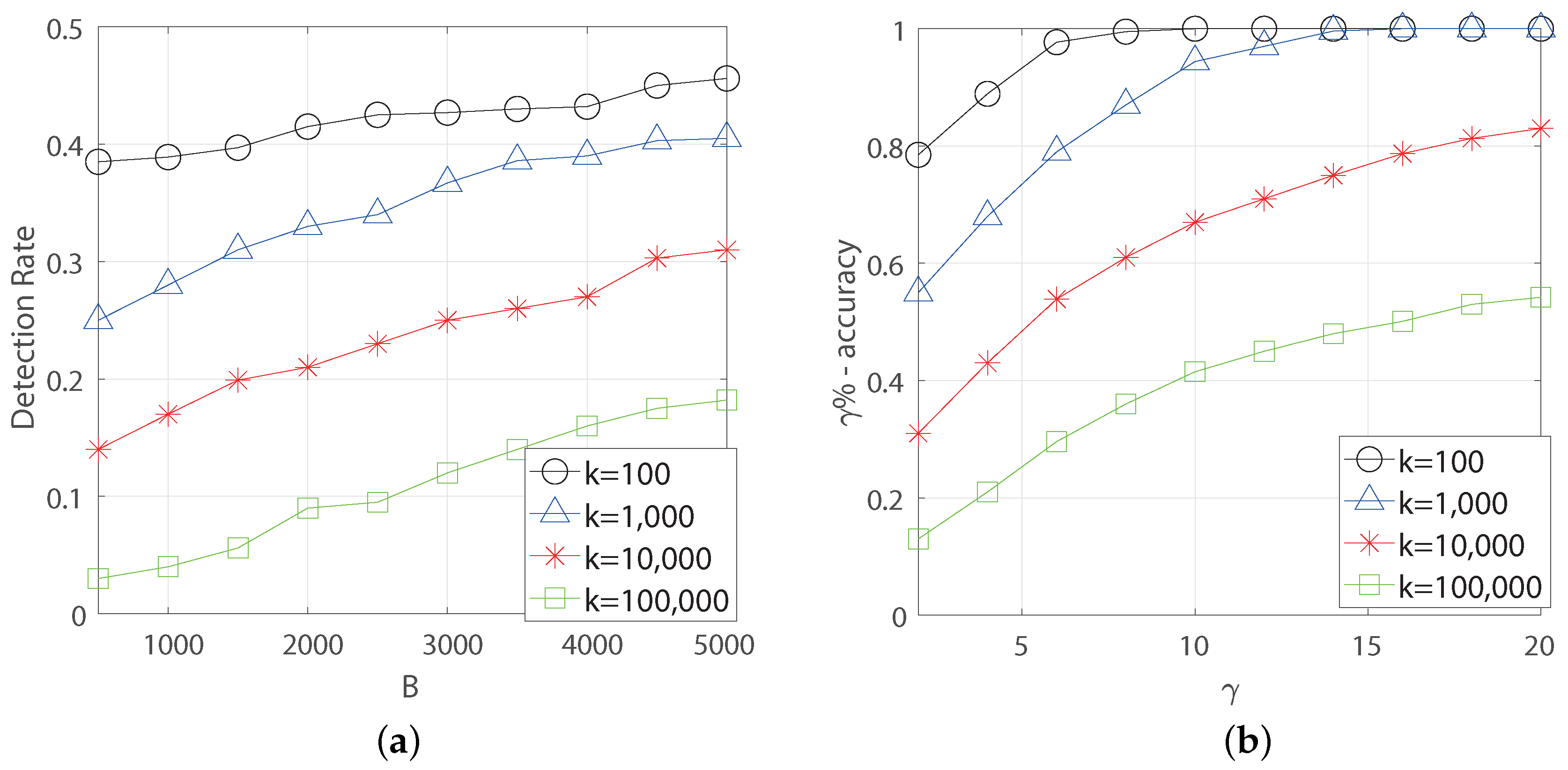
In Figure 3, we first obtain the detection performance for various values $k.$ To do this, we set the flipping parameter $p=0.3$ and diffusion parameter $q=0.4$. In Figure 3a, we obtain the detection probability for $k={10}^2,{10}^3,{10}^4,{10}^5$ by increasing the budget of investigation $B=[500,5000].$ For example, if $k=$ 100,000, about 20% of connections are selected and flip their state with probability p in the network simultaneously at each time step. As a result, we see that for $k=100$, the detection probability increases up to 0.5 when we use the budget $B=5000$. This is because of the portion of selected connection pairs quite low, which means the network remains as an initial ER random graph with high probability. The used source estimator ${\widehat{v}}_{\mathtt{dns}}$ is known that it has a good performance for ER random graph in [14]. For large $k,$ the overall detection performance degraded due to high changes of connections. However, we see that if we use the investigation budget up to 5000, the detection probability increases up to 0.2 even for $k=$ 100,000. This is due to the reconstruction of the contact network by considering the dynamic model with diffusion flow in the network in our algorithm. In Figure 3b, we obtain the $\gamma$%-accuracy for $\gamma \in [2,20]$ using the investigation budget $B=5000$. We see that for $k=100,$ the source is at least top 10% with probability one among the infected nodes whereas it is included in the top 10% with probability 0.4 for $k=$ 100,000. For $k=1000$, the probability that the source is in the top 10% was above 0.9. This comes from the effect of reconstruction of the contact graph using the budget as well as the proper estimator for the source in the algorithm. Finally, we obtain the detection probabilities for various estimation algorithm as described in the earlier subsection in

Table 2. Detection probability of DNSE(k) compared to other methods by varying k. We use the flipping parameter $p=0.3$ and investigation budget $B=2500$.

k	DNSE	JC	RC	NE	DI	DC
${10}^1$	0.49	0.21	0.22	0.31	0.33	0.17
${10}^2$	0.41	0.17	0.19	0.27	0.31	0.14
${10}^3$	0.35	0.14	0.16	0.21	0.27	0.09
${10}^4$	0.21	0.11	0.12	0.18	0.23	0.06
${10}^5$	0.12	0.06	0.09	0.14	0.18	0.03

by increasing $k.$ We use the dynamic parameter $p=0.3$ and investigation budget $B=2500$. We see that our proposed algorithm outperforms others even though all estimators are used after the contact graph reconstruction step in our algorithm. This is because the reconstructed contact graph is good for the estimator in the DNSE(k), which uses the node degree information, i.e., high contact makes a large degree of the node and this promote the flow of information or virus with high probability.

4.3. Effects of Connection Parameter P

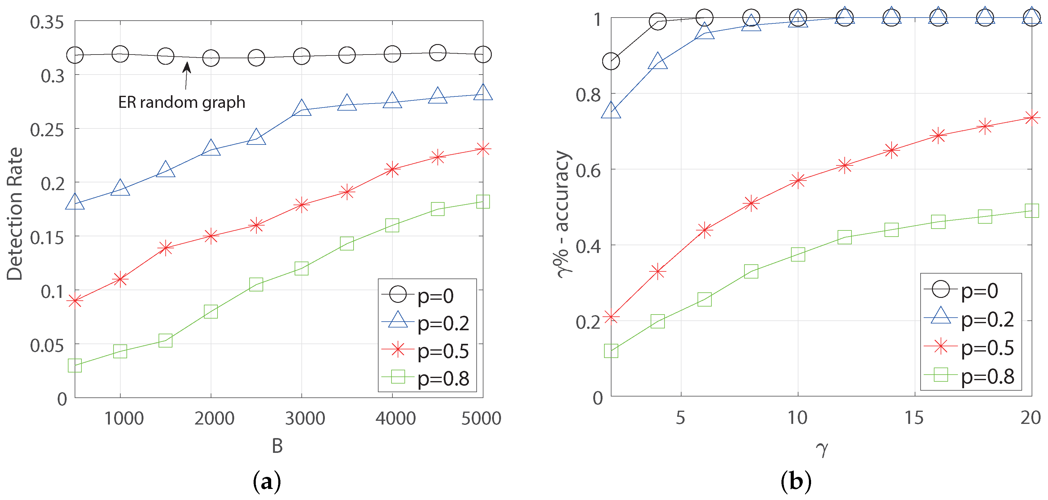
In Figure 4, we obtain the detection performance for various flipping probability $p.$ For the simulation, we set the dynamic parameter $k=5000$ and diffusion parameter $q=0.4$. In Figure 4a, we obtain the detection probability for $p=0,0.2,0.5,0.8$ by increasing the budget of investigation $B=[500,5000].$ If $p=0$, there is no change of connections in the network regardless of the dynamic parameter k. Hence, it remains as an ER random graph, which is initially generated. In this case, we see that the detection probability is about 0.32 regardless of the budget B due to using the source estimator ${\widehat{v}}_{\mathtt{dns}}$, which was designed for ER random graph in [14]. As increasing $p,$ the overall detection performance degraded due to frequent changes in current connections. However, we see that if we use the investigation budget up to 5000, the detection probability also increases up to 0.2 even for $p=0.8$ by reconstruction of the contact graph. In Figure 4b, we also obtain the $\gamma$%-accuracy. We also check that for the cases $p=0,0.2,$ the source is at least in the top 10% with probability 0.99 among the infected nodes whereas it is included in top 10% with probability 0.38 for $p=0.8.$ Finally, we obtain the detection probabilities for various estimation algorithm as described in the earlier subsection in

Table 3. Detection probability of DNSE(k) compared to other methods by varying p. We use the dynamic parameter $k=5000$, diffusion parameter $q=0.4$, and investigation budget $B=2500$.

p	DNSE	JC	RC	NE	DI	DC
0	0.32	0.17	0.21	0.25	0.23	0.15
0.2	0.26	0.15	0.18	0.22	0.21	0.11
0.4	0.18	0.11	0.14	0.18	0.17	0.08
0.6	0.15	0.09	0.11	0.16	0.13	0.05
0.8	0.12	0.08	0.09	0.11	0.09	0.04

by increasing $p.$ We use the dynamic parameter $k=5000$ and investigation budget $B=2500$ and we see that our proposed algorithm DNSE(k) also outperforms to others.

4.4. Effects of Diffusion Rate Q

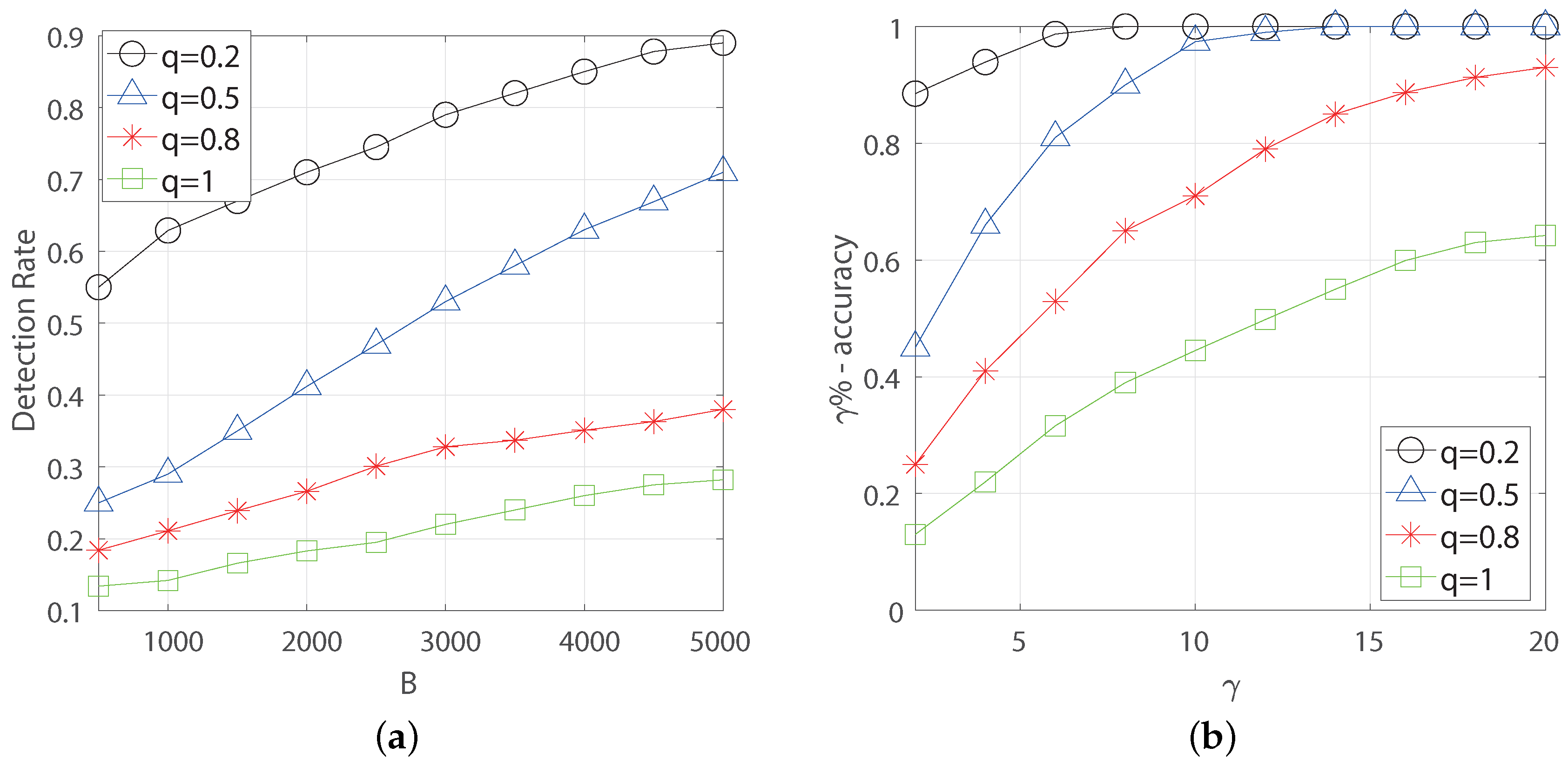
In Figure 5, we obtain the detection performance for various infection probability $q(q=0.2,0.5,0.8,1).$ To do this, we set the flipping parameter $p=0.3$ and dynamic parameter $k=5000$. In Figure 5a, we obtain the detection probabilities by increasing the budget of investigation $B=[500,5000]$ for different q. As a result, we see that for $q=0.2,$ the detection probability increases up to 0.9 when we use the budget $B=5000.$ This is because the number of infected nodes is small by terminating the diffusion process with high probability. For large $q,$ the overall detection performance degraded due to the increasing number of infected nodes in the network. However, if we use the investigation budget up to 5000, the detection probability increases up to 0.3 even for $q=1.$ In Figure 5b, we obtain the $\gamma$%-accuracy for $B=3000$. We also check that for $q=0.2,$ the source is at least in the top 10% with probability one among the infected nodes whereas it is included in top 10% with probability 0.43 for $q=1.$ Finally, we obtain the detection probabilities for various estimation algorithms as described in the earlier subsection in

Table 4. Detection probability of DNSE(k) compared to other methods by varying q. We use the dynamic parameter $p=0.3$ and investigation budget $B=2500$.

q	DNSE	JC	RC	NE	DI	DC
1	0.22	0.06	0.07	0.15	0.13	0.15
0.8	0.31	0.19	0.20	0.27	0.21	0.21
0.6	0.45	0.33	0.32	0.38	0.37	0.28
0.4	0.56	0.45	0.49	0.46	0.53	0.35
0.2	0.81	0.56	0.61	0.51	0.71	0.44

by increasing $q.$ We use the dynamic parameter $k=5000$, flipping parameter $p=0.3$, and investigation budget $B=2500$. The result shows that our proposed algorithm DNSE(k) outperforms to others even though all estimators are used after the contact graph reconstruction step in our algorithm.

4.5. Limitation and Future Works

Most works [2,5,7,8,10,15,25] for static networks design some efficient inference algorithms for detecting the source using the current diffusion snapshot information. Unlike the static network, it is hard to find the diffusion source under the dynamic network due to the loss of information of diffusion history from changing the connections. Hence, tracking or reconstructing the past connection is a fundamental issue in the source estimation problem over the dynamic network. However, if the infected nodes have some side information of the diffusion such as id of the parent node (the node who spreads the information to her) as in [13] or contact node information (our work), a proper query process or some investigation enables us to improve the detection performance by using this information properly.

As future works, some theoretical results of our proposed algorithm can be concerned such that how many investigations will be sufficient to reconstruct the contact graph and study the effects on the performance guarantee for finding the source using the algorithm. Further, it also remains to find a more efficient or an optimal algorithm for reconstructing the contact information for estimation the source in a more practical dynamic setting. For example, from the fact that a single contact does not completely guarantee the flow of information, the graph is recovered from multiple times of contacts. However, as in the example of COVID-19, tracking the contact information requires many resources, so an appropriate trade-off analysis also will be one of the important work in future research. Finally, some of hidden information scenarios should be studied because some of the contact information is hard to obtain by the investigation, which includes the cases that the nodes may not reveal the true information or some nodes cannot be investigated (hidden contact information).

5. Conclusions

In this paper, we consider an epidemic source detection problem under the dynamic network where the connections are changed over time. We design a proper estimation algorithm using some investigation for the true contact information between infected nodes, named by DNSE(k), where the k connections can be changed with some probability at each time. To do that, we use some investigation process to obtain the contact graph between nodes which has a possibility of propagation of the information, and we perform various simulation using this algorithm compared to exciting several source estimation methods. As a result, we see that our proposed algorithm’s detection probability can be above 45% when we use the budget to investigate the contact information between infected nodes under some practical setting of k. Further, our results show that the proposed algorithm outperforms and efficient for finding the epidemic source under the considered dynamic network.

References

1. Hu, Z.; Shen, Z.; Cao, S.; Podobnik, B.; Yang, H.; Wang, W. Locating multiple diffusion sources in time varying networks from sparse observations. Nat. Sci. Rep. 2018, 8, 2685. [Google Scholar] [CrossRef] [PubMed]
2. Shah, D.; Zaman, T. Detecting Sources of Computer Viruses in Networks: Theory and Experiment. In Proceedings of the ACM SIGMETRICS International Conference on Measurement and Modeling of Computer Systems, New York, NY, USA, 14–18 June 2010. [Google Scholar]
3. Shah, D.; Zaman, T. Rumor Centrality: A Universal Source Detector. In Proceedings of the 12th ACM SIGMETRICS/PERFORMANCE Joint International Conference on Measurement and Modeling of Computer Systems, London, UK, 12–14 June 2012. [Google Scholar]
4. Shah, D.; Zaman, T. Rumors in a Network: Who’s the Culprit? IEEE Trans. Inf. Theory 2011, 57, 5163–5181. [Google Scholar] [CrossRef] [Green Version]
5. Zhu, K.; Ying, L. Information Source Detection in the SIR Model: A Sample Path Based Approach. In Proceedings of the IEEE Information Theory and Applications Workshop (ITA), San Diego, CA, USA, 10–15 February 2013. [Google Scholar]
6. Zhu, K.; Ying, L. A robust information source estimator with sparse observations. In Proceedings of the IEEE INFOCOM, Toronto, ON, Canada, 27 April–2 May 2014. [Google Scholar]
7. Wang, Z.; Dong, W.; Zhang, W.; Tan, C.W. Rumor source detection with multiple observations: Fundamental limits and algorithms. In Proceedings of the ACM SIGMETRICS, Austin, TX, USA, 16–20 June 2014. [Google Scholar]
8. Dong, W.; Zhang, W.; Tan, C.W. Rooting Out the Rumor Culprit from Suspects. In Proceedings of the IEEE International Symposium on Information Theory (ISIT), Istanbul, Turkey, 7–12 July 2013. [Google Scholar]
9. Choi, J.; Shin, J.; Yi, Y. Information Source Localization with Protector Diffusion in Networks. IEEE/KICS J. Commun. Netw. 2017, 21, 136–147. [Google Scholar] [CrossRef]
10. Choi, J.; Moon, S.; Woo, J.; Son, K.; Shin, J.; Yi, Y. Rumor Source Detection under Querying with Untruthful Answers. In Proceedings of the IEEE INFOCOM, Atlanta, GA, USA, 1–4 May 2017. [Google Scholar]
11. Choi, J.; Yi, Y. Necessary and Sufficient Budgets in Information Source Finding with Querying: Adaptivity Gap. In Proceedings of the ISIT, Vail, CO, USA, 17–22 June 2018. [Google Scholar]
12. Karsai, M.; Perra, N.; Vespignani, A. Time varying networks and the weakness of strong ties. Sci. Rep. 2014, 4, 4001. [Google Scholar] [CrossRef] [PubMed]
13. Jiang, J.; Wen, S.; Yu, S.; Xiang, Y.; Zhou, W. Rumor Source Identification in Social Networks with Time-Varying Topology. IEEE Trans. Dependable Secur. Comput. 2018, 15, 166–179. [Google Scholar] [CrossRef]
14. Zhu, K.; Ying, L. Information Source Detection in Networks: Possibility and Impossible Results. In Proceedings of the IEEE INFOCOM, San Francisco, CA, USA, 10–15 April 2016. [Google Scholar]
15. Prakash, B.A.; Vreeken, J.; Faloutsos, C. Spotting Culprits in Epidemics: How Many and Which Ones? In Proceedings of the IEEE International Conference on Data Mining, Brussels, Belgium, 10–13 December 2012. [Google Scholar]
16. Fioriti, V.; Chinnici, M.; Palomo, J. Predicting the Sources of an Outbreak with a Spectral Technique. Appl. Math. Sci. 2014, 8, 6775–6782. [Google Scholar] [CrossRef] [Green Version]
17. Bubeck, S.; Devroye, L.; Lugosi, G. Finding Adam in random growing trees. Random Struct. Algorithms 2017, 50, 158–172. [Google Scholar] [CrossRef] [Green Version]
18. Khim, J.; Loh, P.-L. Confidence Sets for Source of a Diffusion in Regular Trees. IEEE Trans. Netw. Sci. Eng. 2015, 4, 27–40. [Google Scholar] [CrossRef] [Green Version]
19. Luo, W.; Tay, W.P.; Leng, M. How to Identify an Infection Source With Limited Observations. IEEE J. Sel. Top. Signal Process. 2014, 8, 586–597. [Google Scholar] [CrossRef] [Green Version]
20. Prakash, B.A.; Vreeken, J.; Faloutsos, C. Efficiently Spotting the Starting Points of an Epidemic in a Large Graph. In Proceedings of the ICDM, New Orleans, LA, USA, 18–21 November 2017. [Google Scholar]
21. Zhu, K.; Chen, Z.; Ying, L. Catch’Em All: Locating Multiple Diffusion Sources in Networks with Partial Observations. In Proceedings of the AAAI, San Francisco, CA, USA, 4–9 February 2017. [Google Scholar]
22. Ji, F.; Tay, W.P. An Algorithmic Framework for Estimating Rumor Sources with Different Start Times. IEEE Trans. Signal Process. 2017, 65, 2517–2530. [Google Scholar] [CrossRef]
23. Michael, F.; Yu, P.-D. Rumor source detection for rumor spreading on random increasing trees. Electron. Commun. Probab. 2015, 20, 2. [Google Scholar]
24. Woo, J.; Choi, J. Estimating the Information Source under Decaying Diffusion Rates. Electronics 2019, 8, 1384. [Google Scholar] [CrossRef] [Green Version]
25. Chang, B.; Zhu, F.; Chen, E.; Liu, Q. Information source detection via Maximum A postreia Estimation. In Proceedings of the IEEE ICDM, Atlantic City, NJ, USA, 14–17 November 2015. [Google Scholar]
Figure 1. Example of movement of information source over dynamic network. (Red: infected node, S: Source).
Electronics 09 01018 g001
Figure 2. Illustration of the algorithm Dynamic Network Source Estimation (DNSE)(k). (In the initial step, the network consists of three disconnected subnetworks. Choose k t = 3 to investigate of contact and, if true, connect an edge between node pairs. Repeat this procedure until finishing the investigation and finally estimate the source in the final step.)
Electronics 09 01018 g002
Figure 3. Detection rate and γ %-accuracy of DNSE(k) for various dynamic parameter k . (we set the flipping parameter p = 0.3 and diffusion parameter q = 0.4 , respectively.) (a) Detection rate vs. Budget B. (b) γ %-accuracy.
Electronics 09 01018 g003
Figure 4. Detection rate and γ %-accuracy of DNSE(k) for various flipping parameter p . (we set the dynamic parameter k = 5000 and diffusion parameter q = 0.4 , respectively.) (a) Detection rate vs. Budget B. (b) γ %-accuracy.
Electronics 09 01018 g004
Figure 5. Detection rate and γ %-accuracy of DNSE(k) for various diffusion parameter q . (we set the flipping parameter p = 0.3 and dynamic parameter k = 5000 .) (a) Detection rate vs. Budget B. (b) γ %-accuracy.
Electronics 09 01018 g005