Article

Multiband SHEPWM Control Technology Based on Walsh Functions

College of Electrical and Automation Engineering, East China Jiaotong University, Nanchang 330013, China
*
Author to whom correspondence should be addressed.
Electronics 2020, 9(6), 1000; https://doi.org/10.3390/electronics9061000
Submission received: 7 May 2020 / Revised: 4 June 2020 / Accepted: 10 June 2020 / Published: 15 June 2020
(This article belongs to the Section Systems & Control Engineering)

Abstract

:
The drawback of modulation ratio limitation in selective harmonic elimination pulse width modulation (SHEPWM) technology based on Walsh function transformation. In order to solve this problem, a multiband SHEPWM control technology method for a multilevel inverter based on Walsh functions is proposed. By analyzing multiband SHEPWM for multilevel inverter voltage waveforms under a Fourier series transform, the unified nonlinear multiband SHEPWM equations for a multilevel inverter with a modulation index varying from 0 to 1 can be generalized. The equations can be solved by Walsh function transform. In this way, the difficulties faced in expanding the modulation index, online calculation, and real-time control are resolved simultaneously. A seven-level inverter is taken as the example, for which the piecewise linear equations of Walsh functions under different bands and the trajectories of switching angles are given. Meanwhile, the conditions for multiple sets of solutions at such a point where the modulation index is switched over are also taken into account. The feasibility of the proposed method is verified by simulation based on MATLAB and SIMULINK. Finally, the feasibility of the practical application is proved by the experiment based on Digital Signal Processor (DSP).

1. Introduction

The cascaded H-bridge (CHB) multilevel inverter is one of the popular converter topologies used in high-power medium-voltage (MV) drives [1]. It has many advantages, such as its high voltage level, low voltage change rate, and its easy modularization [2]. The pulse width modulation schemes for multilevel inverters can be generally classified into carrier-modulated sine pulse width modulation (SPWM) [3], voltage space vector pulse width modulation (SVPWM) [4], and selected harmonics elimination pulse width modulation (SHEPWM) [5,6,7]. The SHEPWM scheme has several distinct advantages, such as having a low switching frequency, high output quality, low switching losses, and high inverter efficiency. The core issue of the SHEPWM control is the solution of nonlinear equations of the multilevel inverter, including the selection of initial values and the selection of iterative algorithms. In addition, the traditional trapezoid wave modulation SHEPWM for multilevel inverter control technology is limited by the modulation index, which generally cannot randomly change from 0 to 1. When the modulation index is relatively low, the SHEPWM nonlinear equations may have no solutions.
At present, most papers use the Newtonian iterative method to solve nonlinear equations, but this needs to find the initial value, which is relatively close to the accurate value, in order to make the algorithm converge, otherwise the iterative algorithm is be convergent. The polynomial synthesis method and the power method are proposed to solve nonlinear equations in [4,5]. However. these methods are too complicated and need to be derived for different levels, which makes it hard for them to be widely used. The homotopic algorithm is applied to solve the SHEPWM nonlinear equations in [7], which raises the rate of convergence of the iterative process to a certain extent. However, the dependence on the initial value of the iterative process is still strong and there is no guarantee that the iteration can be convergent. A SHEPWM function is proposed based on the Walsh functional transform in [8] by analyzing the relationship between the Walsh domain and the Fourier domain, and by transforming the nonlinear transcendental equations of the Fourier domain into the Walsh function under the domain of the piecewise linear system of equations. The calculation steps of the conversion process are improved and the recursive methods used between the harmonic elimination angles and the fundamental wave voltage section amplitude are proposed in [9,10,11,12].
To obtain the initial value, the trial and error method is used in [8]. If there is a lack of evidence when selecting the initial value, the efficiency of the iteration is low. Sometimes equations may also be divergent. The triangular carrier SPWM method is used to get the initial solution in [9]. In fact, this is the method used to solve the reference sine function and a series of piecewise linear functions. However, the calculation process is very troublesome. The approach of Wu is introduced to find the solutions for the initial values of the SHEPWM nonlinear equations in [10], which is complex and hard to achieve.
To expand the modulation index of SHEPWM for a multilevel inverter, the method of reducing a pulse to extend the modulation index to 0.2 is used in [11]. However, the freedom degrees and the number of harmonics eliminated will be reduced at the same time. The polarity reverse method is proposed to expand the modulation index in [12], however the energy consumption control of the DC link needs to be increased to solve the problem of the energy feedback caused by its structure. The six sections of the ladder-type wave switching model are proposed in [13], but the problem of the energy feedback also exists and the working frequency of the switch cannot stay the same.
As it is easy to solve nonlinear equations by using Walsh functions and they have a low dependence on the initial solution, a kind of transformation method is proposed, for which the multilevel inverter modulation index of the multiband SHEPWM modulation scheme [14] can be broadened and combined with Walsh functions. The SHEPWM voltage waveforms of the multilevel inverter in different waveform band modes are analyzed and the multiband SHEPWM solution model with modulation indexes ranging from high to low is established. Finally, the unity SHEPWM equations of the piecewise linear system of equations can be solved using the Walsh function transformation.
This paper is organized as follows: The harmonic elimination model of the multiband SHEPWM is presented in Section 2. Section 3 introduces the Walsh function. The Walsh function transform is proposed to solve the angle of the multiband equation in Section 4. Simulations and experimental results are presented in Section 5 and Section 6, respectively, to validate the performance of the proposed method. Finally, the conclusions are summarized in Section 7.

2. Harmonic Elimination Model for Multiband SHEPWM

The topology structure of the H-bridge cascaded seven-level inverters is shown in Figure 1. It is composed of a series connection of three H-bridge cells. Each H-bridge unit is powered by a separate DC power supply. Assuming that the input voltages of the three H-bridge cells are Vdc1 = Vdc2 = Vdc3 = E, the corresponding output voltages of each cell are VH1, VH2, VH3. The generated output voltage of each cell is composed of the three voltage levels +E, −E, and 0, using a different combination of the four switches.
Table 1 shows the output voltage of the inverter under different output functions. Where S1, S2 and S3 are the output level function of H1, H2 and H2 respectively. It can be seen from the table that the phase voltage VAN of the three-element CHB inverter canh1 have a total of seven levels of ±3E, ±2E, ±E, and 0. In order to avoid energy circulation, the output states of the opposite polarity of the output voltage of each unit are removed in Table 1. It can be seen from the table that when the output levels of the phase voltage VAN are ±2E and ±E, each unit has a redundant output state function.
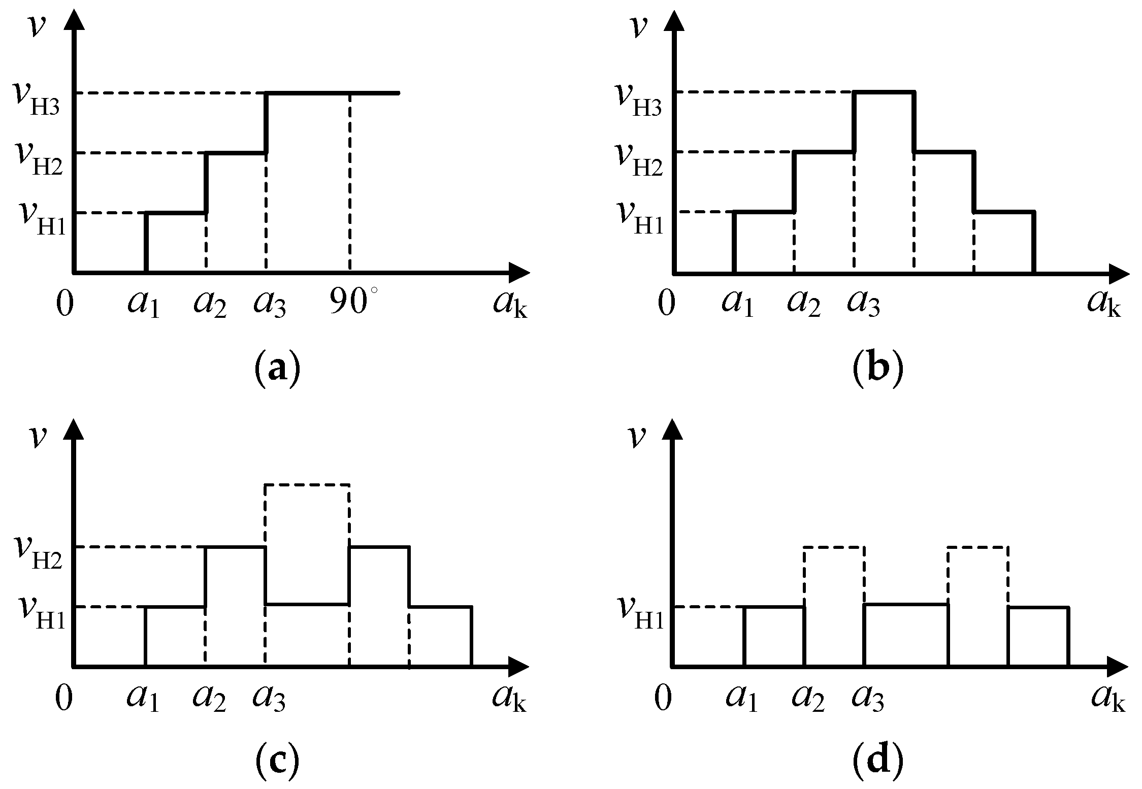
The multiband SHEPWM multilevel inverter waveform is shown in Figure 2.
The graph of the seven−level phase voltage is shown in Figure 2a, which is transformed by a Fourier transform as follows:
u ( t ) = c 0 + n = 1 ( c n cos ( n ω t ) + b n sin ( n ω t ) )
where
{ c 0 = 1 T 0 T u ( t )   d t c n = 2 T 0 T u ( t ) cos ( n ω t )   d t , n = 1 , 2 , 3
Expanding and analyzing bn in Equation (1) we get:
u ( ω t ) = { b n = 0 ,          n is even b n = 4 E n π k = 1 N p k cos ( n θ k ) , n i s o d d
The switching angles denoted by θ k (in radians) are 0 0 θ 1 < θ 2 < < θ N 90 0 . Here, E is the voltage value for each unit of dc; bn is the harmonic coefficient; pk is marked + 1 when it rises at the point of θ k and −1 when it decline. The graph of the half-wave symmetry waveform of the seven-level ladder-type modulation is shown in Figure 2b, in which the output voltages of each unit H-bridge are VH1, VH2, and VH3. According to Equation (3), a harmonic elimination of nonlinear equations can be established. There are no solutions when the modulation index is lower than 0.4, as the five- and seven-fold harmonics are eliminated by the numerical algorithm. According to the above situation, a multiband modulation scheme is proposed in this paper by broadening the index of modulation. The modulation index can be broadened as shown in Figure 2c,d.
By observing the staircase waveform, it is easy to find that the waveform transformation rules between different wavebands are used to fold down the waveform with the dotted line at the top. The applicable modulation indexes shown in Figure 2b to Figure 2d for modulation modes A, B, and C are [0.4, 1], [0.3, 0.3], and [0, 0.3], respectively. The modulation index can be broadened to 0–1 according to the above multiband modulation method. The correct switch angles under different modulation indexes can be obtained by establishing SHEPWM nonlinear equations in accordance with the waveforms of different wavebands, for which the modulation index has different ranges.

3. Walsh Functions

The Walsh function is a standard orthogonal function system. It has only two values, 0 and 1, but the value of the function changes between 0 and 1, so the theoretical analysis is more complex than the trigonometric function. In recent years, due to the rapid development of new disciplines and technologies, Walsh function theory has been widely used in radar, communication, medicine, imaging, and other fields. The introduction of the Walsh function into the electrical field is of great significance.
The Walsh functions are a set of complete orthogonal function systems that can be expressed as Wal(n,t), where n is usually the zero crossing point (ZCP) number under time T of a certain order for the definition of Walsh functions, where t is the normalized time spacing of T.
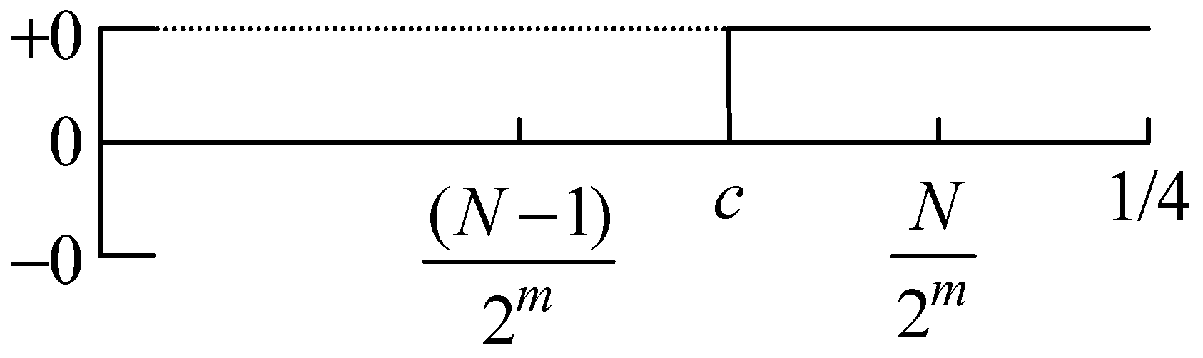
The quarter-cycle waveform normalized by Figure 2a is shown in Figure 3, where T (0–1) is divided into 2m uniform areas, c is the normalized value of θ1, and the interval number of the rising edge is marked with N. Similar to Fourier expressions, the Walsh functions are obtained using the waveform transformed by the Walsh function, which are shown below:
f ( t ) = a 0 + W a 1 ( 0 , t ) + i = 1 N 1 a i W a 1 ( i , t )
{ a 0 = 2 T 0 T f ( t ) W a 1 ( 0 , t ) d t ,   i = 1 , 2 , 3 , a 1 = 1 T 0 T f ( t ) W a 1 ( i , t ) d t ,   i = 1 , 2 , 3 ,
Equation (4) is simplified according to the symmetry as follows:
f ( t ) = i = 1 N / 2 W 4 i 3 W a 1 ( 4 i 3 , t )
In Equation (6), W 4 i 3 = F w ( 4 i 3 ) is the coefficient of W a 1 ( 4 i 3 , t ) , meaning that the corresponding waveform of the Walsh functions is f(t). A quarter cycle of the normalized three-level PWM waveform is shown in Figure 2. According to Figure 2, Equation (7) can be deduced as follows:
F w ( 4 i 3 ) = 0 1 f ( t ) W a 1 ( 4 i 3 , t ) d t = 1 2 m 2 n = N + 1 2 m / 4 W a 1 ( 4 i 3 , n ) + ( N 2 m 2 4 c ) W a 1 ( 4 i 3 , N ) ,   i = 1 , 2 , 3 ,
As seen in Equations (1) and (4), some transformations can be taken to convert the transcendental equations under the domain of the Fourier transform into piecewise linear equations under the domain of the Walsh function. According to the Equation (3), we can get:
u ( w t ) = f ( w t ) = n = 1 b 2 n 1 sin [ ( 2 n 1 ) w t ]
b 2 n 1 = 8 π 0 π / 4 f ( w t ) sin [ ( 2 n 1 ) w t ] d ( w t ) , n = 1 , 2 , 3 ,
Under the same angular frequency, Equation (6) can be developed under the domain of the Walsh function to infinity, Equation (8) can be made equivalent with it under the Fourier transform, then Equation (6) can be brought into Equation (9), and we can get:
b 2 n 1 = 8 π 0 π / 4 i = 1 W 4 i 3 W a 1 ( 4 i 3 , w t ) sin [ ( 2 n 1 ) w t ] d ( w t ) , n = 0 , 1 , 2 , 3 ,
Assuming that:
B 2 n 1 ( W a 1 ( 4 i 3 , w t ) ) = 8 π 0 π / 4 W a 1 ( 4 i 3 , w t ) sin [ ( 2 n 1 ) w t ] d ( w t )
Equation (11) is the Fourier coefficient of the (2n−1) harmonic for the Walsh function W a 1 ( 4 i 3 , w t ) , then we plug in Equation (10) into the deformation:
b 2 n 1 = i = 1 W 4 i 3 B 2 n 1 [ W a 1 ( 4 i 3 , w t ) ]
Equation (11) is complex to solve, while a nonrecursive formula of the Walsh function Fourier transformation is given in [15,16]. For k = 2i−1, i = 1,2,3,…, m = 4n−3, n = 1,2,3,…:
B k ( W a 1 ( m , w t ) ) = 2 ( 1 ) g 0 ( j ) d × [ x = 0 M 1 cos ( π k 2 x + 1 π g x 2 ) ] sin ( π k / 2 M ) π k / 2 M
In which j = (−1)1/2 records only plus or minus of (−j)d when calculating, while the variable instructions of Equation (13) are as follows:
  • Record the order of the Walsh function as m, making its expressions for e binary;
  • Convert e as gray code g, the record the x bite of the gray code for gx;
  • M is the total number of g, while d is the total number of 1 contained in g.

4. Solving Equations

Summarizing Equation (11):
[b] = [U] = [B][F]
In this process, [b] is the harmonic coefficient matrix, which is replaced by [U] for simplification. The matrixes [B] and [F] are the Walsh transform matrix and Walsh coefficient matrix.
We assume that the harmonic coefficient Uk of the k time eliminated harmonic component is zero, which satisfies the fundamental current amplitude at the same time. We then establish a harmonic elimination system for linear equations and solve the switch angle, the calculation steps for which are shown as follows:
  • Determine the total interval number N according to the precision of the harmonic elimination, give a set of relatively accurate initial values, determine the interval after normalization, and serve the initial conditions;
  • According to interval number N and the harmonic number k, calculate the Walsh transform matrix [B];
  • According to interval number N and the determined initial conditions, calculate the Walsh coefficient matrix [F];
  • According to Equation (14), establish the piecewise linear system of equations;
  • Solve the piecewise linear system of equations and get the corresponding number of switch angles.
Taking the seven-level waveband A as an example, the accuracy of the interval number N is shown as 64 [16], the initial switch angles for a1, a2, and a3 are 11.52°, 28.728°, and 57.096°. The interval numbers of the switch angles are 3, 6, and 11, respectively. The scope of the initial angles is shown as:
2 × 360/64 ≤ a1 ≤ 3 × 360/64, 5 × 360/64 ≤ a2 ≤ 6 × 360/64, 10 × 360/64 ≤ a3 ≤ 11 × 360/64
For the seven-level inverter’s three-phase system, five and seven-fold harmonics are generally eliminated. The Walsh coefficient matrix [F] can be obtained by the selection of the initial conditions and by using Equation (7), as shown in Table 2. The corresponding coefficient of the Walsh function is Fw(4i3), where i = 1,2,3…, and using the interval number N and the eliminated harmonic number k, the Walsh transform matrix [B] can be obtained, as shown in Table 3. As space is limited, only some of the data are shown.
Combined with Equation (14):
U1 = 4.5327 − 1.9431a1 − 4.1112a2 − 6.8591a3, U5 = − 0.6268 − 7.4570a1 − 3.3862a2 + 7.1595a3,
U7 = 0.8745 − 7.7586a1 + 4.6724a2 − 6.3000a3
Assuming that the harmonic coefficients U5 and U7 are zero, according to Equation (16):
a1 = −0.0140U1 + 0.0748, a2 = −0.1186U1 + 0.4422, a3 = −0.0707U1 + 0.3746
According to Equations (15) and (17), we get 1.4172 ≤ U1 ≤ 1.4523, which meets the fundamental current amplitude conditions. Thus, the first set of solutions can be obtained. Then, the limit value, which met Equation (17), should be substituted into Equation (16), and the other set of switch angles can be obtained. After determining the range, the process above can be repeated and another set of solutions can be obtained. All switch angles can also be obtained.
Taking the seven-level inverter multiband ladder-type modulation as an example, the switching angles for SHEPWM can be solved using Walsh transforms. The selected interval number N is 64 and the eliminated 5th and 7th harmonic are calculated in accordance with the above example. Along with the multiband modulation mode, as shown in Figure 2, the harmonic elimination switch angles of A, B, and C mode can be obtained, as shown in Table 4, Table 5 and Table 6.
The linear equations transformed by Walsh functions cannot be solved when the seven-level inverter modulation index of 64 under the C band mode is below 0.170, as shown in Table 5. To solve this problem, the solution involving expanding the interval number is adopted, so that the interval number N is taken as 128 and the C band mode switch angles can be evaluated, as shown in Table 7.
As is known, after the interval number N changes from 64 to 128, the number of modulation segments increases dramatically. To get a lower modulation index for the switch angles, the precision of the switch angles is improved as well, but the calculation is increased with the corresponding computation.

5. Simulation Result

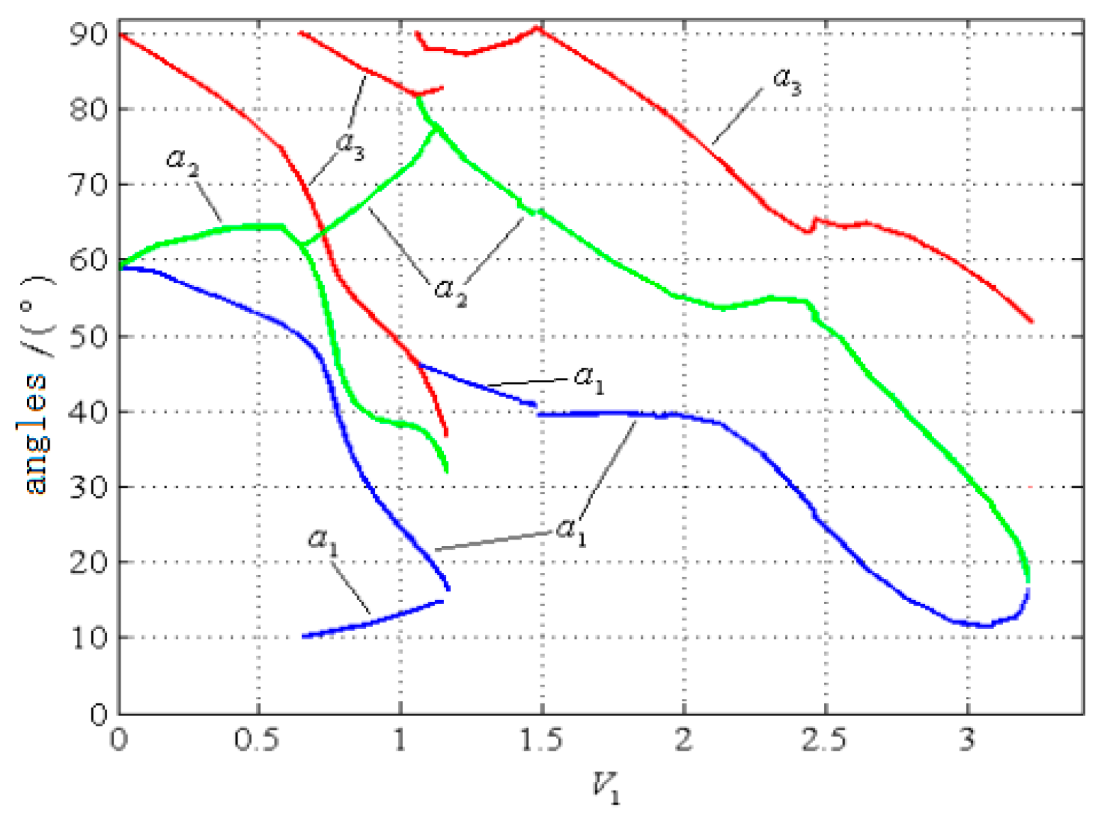
Based on the data in the above tables, this paper draws the change track of the angle of the harmonic elimination switch with the amplitude of the fundamental voltage, as shown in Figure 4.
It can be seen from Figure 4 that the correct switching angle can be obtained for each band of the modulation index in the range of 0–1. Moreover, it can be found that there are multiple sets of switch angle trajectories in each cell near each switch band. These redundant switch angles can increase the flexibility of the switch angle selection and improve the control performance in the actual control.
To test and verify the correctness of the above theoretical analysis and the solving solution, MATLAB and SIMULINK software were used for the seven-level inverter of the multiband SHEPWM based on the Walsh function transform to build the model and do the experiment. The simulation parameters were as follows: the independent dc voltage source was 50; A, B, and C bands took fundamental voltage amplitude U1 as 3.15, 1.32, and 1.0, respectively, when choosing the switch angles. The output voltage waveforms and spectrum distribution are shown in Figure 5, Figure 6 and Figure 7.
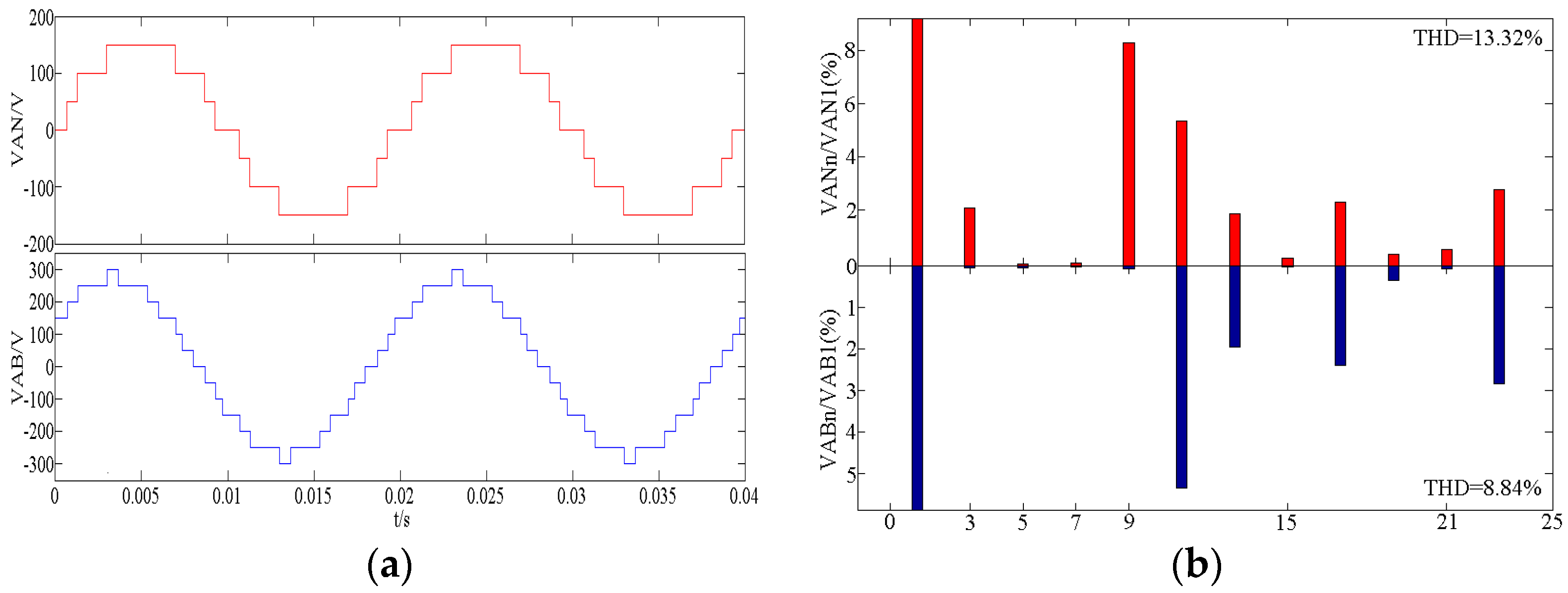
Figure 5 shows the waveform of the output phase voltage VAN and line voltage VAB in the A band when the fundamental voltage amplitude is 3.15, along with the Fast Fourier Transform (FFT) analysis.
Here, VAN is the A phase voltage, VAB is the line voltage, VANi is the A phase voltage harmonic, VABi is the A phase line voltage harmonic, VAN1 is the fundamental wave of the A phase, and VABi is the fundamental wave of the line voltage between phase A and phase B.
According to Figure 5a, it can be seen that the phase voltage VAN is 7 levels and the line voltage VAB is 13 levels, which conforms to the design of the A band. From Figure 5b, it can be seen that the Total Harmonic Distortion (THD) of the phase voltage VAN is 13.32%, in which the 5th and 7th harmonics are eliminated. The THD of the line voltage VAB is 8.84%, in which the 3rd, 5th, and 7th harmonics are eliminated, which proves the correctness of the switch angle calculation. At the same time, a high-quality voltage waveform can be obtained under the SHEPWM modulation.
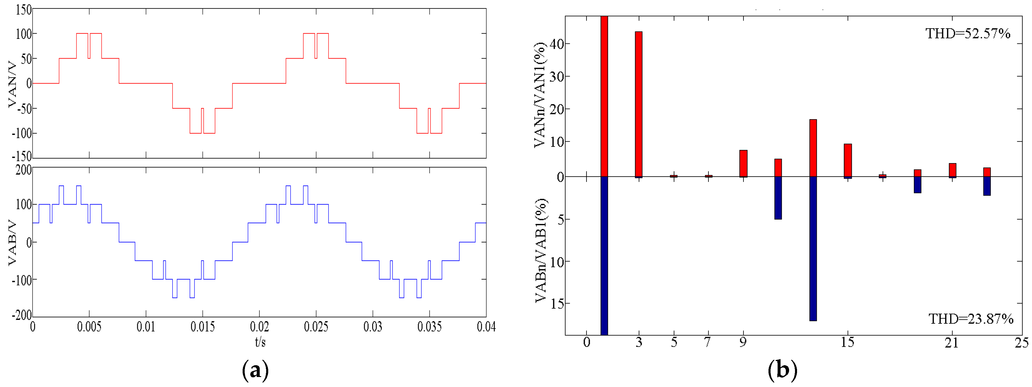
Figure 6 shows the waveform of the output phase voltage VAN and the line voltage VAB in the B band when the fundamental voltage amplitude is 1.32, along with the FFT analysis.
According to Figure 6a, it can be seen that the phase voltage VAN is 5 levels, while the line voltage VAB is 7 levels, which conforms to the design of the B band. From Figure 6b, it can be seen that the THD of the phase voltage VAN is 52.57%, in which the 5th and 7th harmonics are eliminated. The THD of line voltage VAB is 23.87%, in which the 3rd, 5th, and 7th harmonics are eliminated, which proves the correctness of the switch angle calculation.
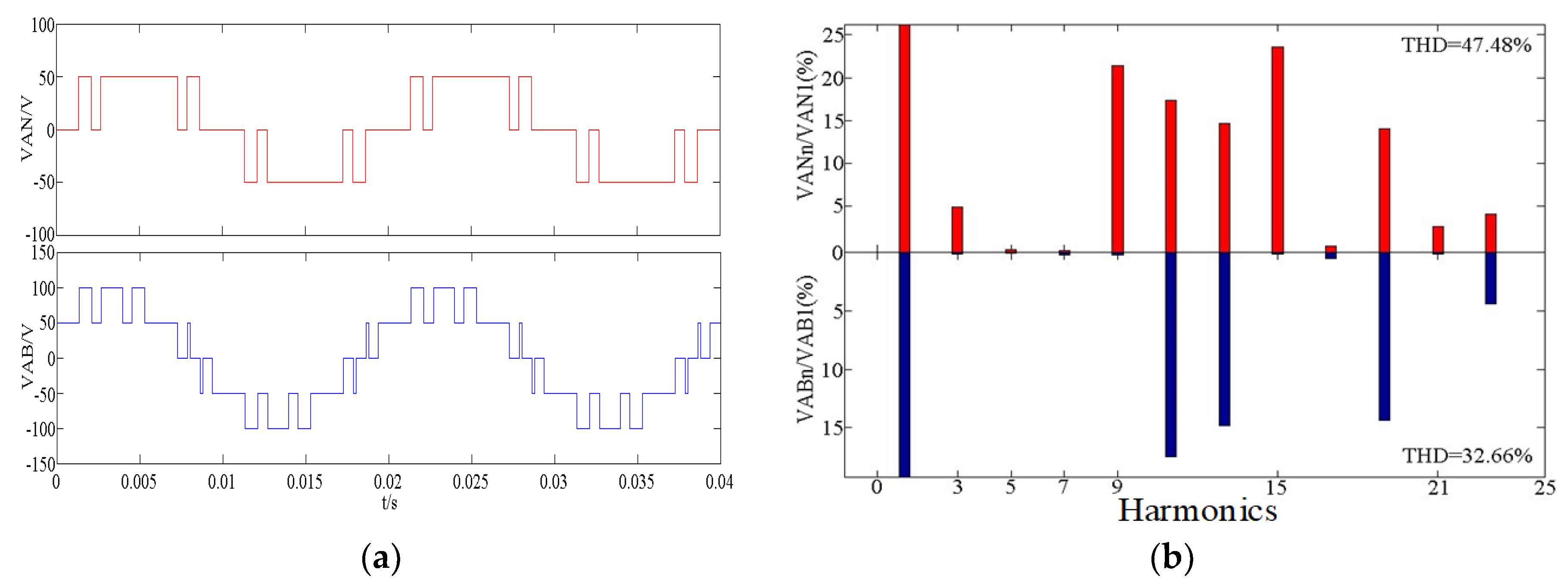
Figure 7 shows the waveform of the output phase voltage VAN and the line voltage VAB in the C band when the fundamental voltage amplitude is 1.0, along with the FFT analysis.
As shown in the Figure 7a, the phase voltage VAN is 3 levels, while the line voltage VAB is 5 levels, which conforms to the design of the C band. From Figure 7b, it can be seen that the THD of phase voltage VAN is 47.48%, in which the 5th and 7thharmonics are eliminated. The THD of line voltage VAB is 32.66%, in which the 3rd, 5th, and 7th times harmonics are eliminated, which proves the correctness of the switch angle calculation.
As shown in Figure 5, Figure 6 and Figure 7, the 5th and 7th harmonics have basically been eliminated, which can be proved using the control technology of the SHEPWM multilevel inverter based on the Walsh transform, combined with multiband modulation, which is feasible in this paper. Because of the limitation of the calculation accuracy and the precision of the numerical algorithm needed to solve the switch angles, the harmonic cannot be completely eliminated. Usually it will have a small amount of deviation, and the calculation of the accuracy of the switch angles under different modulation indexes is not the same.
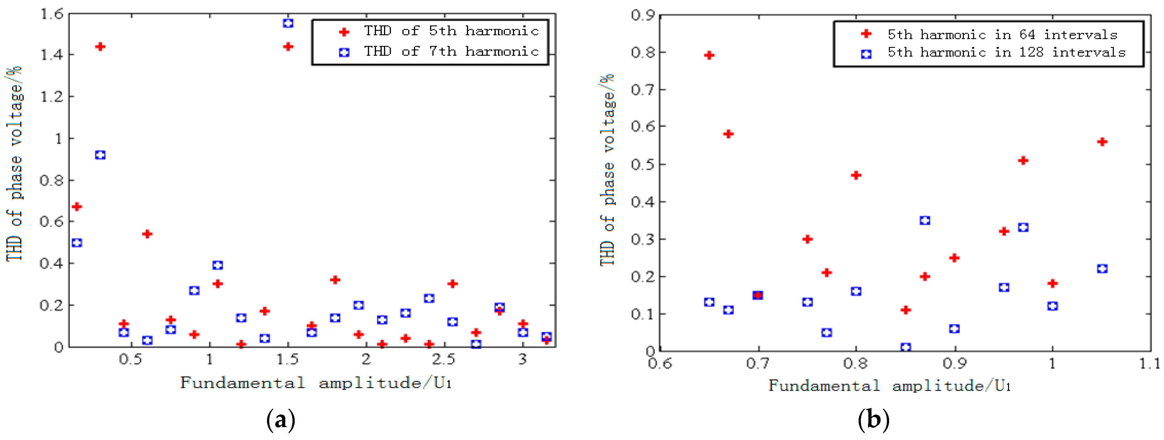
In this paper, the effects on harmonic elimination under various modulations based on multilevel inverters have been studied, and 5th and 7th harmonic indexes have been listed. The amplitudes of 5th and 7th harmonics, which have been completely eliminated, theoretically are actually not zero, as shown in Figure 8a. The 5th harmonic indexes based on 64 and 128 phase voltage interval schemes under the C band model are given in Figure 8b.
As shown in the Figure 8a, although the 5th and 7th harmonics have not been completely eliminated, there is a very small amount of error. The values are different under various modulation indexes. The errors indicate that the switch angles of the SHEPWM are not accurate, but they can be completely ignored in actual engineering control. From Figure 8b, the harmonic indexes in the 128-interval scheme are lower than the 64-interval scheme overall. This proves that the larger the interval scheme that is selected, the more precise the switch angels are and the better harmonic elimination effect it has.

6. Experiment Verification

In order to prove the feasibility of the algorithm proposed above and the harmonic elimination effect in the practical engineering, an inverter experiment platform is set up, whose parameters are reported in Table 8. An interface board is designed to do the isolated signal conditioning required for Analog to Digital Converter (ADC) module of a Digital Signal Processor(DSP)controller. The utilized processor is a TMS320F2812(Texas Instruments, Texas, USA) controller used to perform all necessary functions in the discrete time domain.
The output phase voltage VAN of the inverter under the SHEPWM modulation when the modulation index is 0.75 and its spectrum are shown in Figure 9a,b, respectively. Figure 9c,d show the output phase voltage VAN of the inverter when the modulation is 0.46 and its spectrum, respectively. 
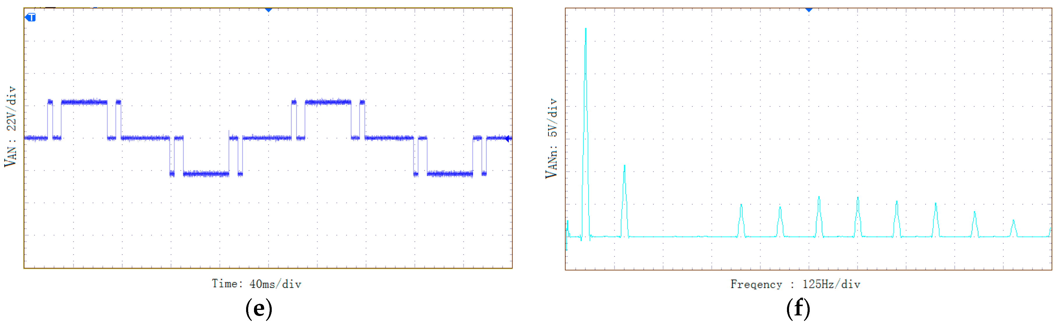
Figure 9e,f show the output phase voltage VAN of the inverter when the modulation is 0.27 and its spectrum, respectively.
When the modulation index is 0.75, it corresponds to the SHEPWM modulation in the A band. Figure 9a shows that the output phase voltage is 7 levels. In addition, Figure 9b shows that the 5th and 7th harmonics are basically eliminated and the THD of the phase voltage VAN is 34.9%.
When the modulation index is 0.46, it corresponds to the SHEPWM modulation in the B band. Figure 9b shows that the output phase voltage is 5 levels. In addition, Figure 9e shows that the 5thand 7th harmonics are basically eliminated and the THD of the phase voltage VAN is 43.1%.
When the modulation index is 0.27, it corresponds to the SHEPWM modulation in the C band. Figure 9c shows the output phase voltage is 3 levels. In addition, Figure 9f shows that the 5th and 7th harmonics are basically eliminated and the THD of the phase voltage VAN is 63.2%.
Overall, the correctness of the switch angle obtained by the multilevel inverter for the multiband SHEPWM control technology based on the Walsh function is proven. In addition, the multiband SHEPWM control technology of the multilevel inverter based on the Walsh function proposed in this paper can solve the problem of the limited modulation index in the specific harmonic elimination PWM technology effectively.

7. Conclusions

The following conclusions can be summarized from the analysis and research for the multiband SHEPWM control method based on the Walsh function transform for the multilevel inverter.
  • By combining the Walsh function transformation with the multiband SHEPWM control method for the multilevel inverter, the regulation operation range of the inverter can be expanded to 0–1. At the same time, the traditional SHEPWM nonlinear equations are transformed into piecewise linear equations, and the online calculation of the switching angle of the SHEPWM multilevel inverter is obtained, which makes real-time harmonic elimination control possible.
  • The switch angles cannot be solved with the fundamental current amplitude, which is below 0.656, by using 64-interval accuracy for the Walsh function transformation, but the switch angles under the lower precision modulation index can be solved by using the 128-interval Walsh function transformation.
  • The simulation results show that the 5th and 7th harmonics of each band modulation mode are nearly eliminated, which proves that the method based on the Walsh function is correct and feasible.

Author Contributions

Project management, M.Y.; conceptualization, G.S.; methodology, G.S. and S.L.; analysis, G.S.; software writing, Q.W.; validation, G.S., W.R., and S.L.; writing—original draft preparation, G.S.; writing—review and editing, M.Y. All authors have read and agreed to the published version of the manuscript.

Funding

This research was funded by National Natural Science Foundation of China, grant number 51767007; Jiangxi Provincial Industrial Science and Technology Support Project, grant number 20192BBEL50011; Jiangxi Natural Science Foundation Project, grant number 20192BAB206036; Jiangxi Provincial Youth Science Foundation of China, grant number GJJ190312.

Conflicts of Interest

There are no conflicts of interest regarding the publication of this paper.

References

  1. Venkataramanaiah, J.; Suresh, Y.; Anup, K.P. Development of a New Hybrid Multilevel Inverter Using Modified Carrier SPWM Switching Strategy. IEEE Trans. Ind. Electron. 2018, 33, 8192–8197. [Google Scholar]
  2. Ye, M.Y.; Nie, Y. Research on photovoltaic grid connected control of three-phase cascade H-bridge. J. East China Jiaotong Univ. 2019, 36, 99–104. [Google Scholar]
  3. Saroj, K.S.; Tanmoy, B. Phase-Shifted carrier-based synchronized sinusoidal PWM techniques for a cascaded H-bridge multilevel inverter. IEEE Trans. Power Electron. 2018, 33, 513–524. [Google Scholar]
  4. Edpuganti, A.; Rathore, A.K. Fundamental switching frequency optimal pulse width modulation of medium-voltage cascaded seven-level inverter. IEEE Trans. Ind. Appl. 2015, 51, 3485–3492. [Google Scholar] [CrossRef]
  5. Sanjiba, K.B.; Nirmal, K.A. SHE-PWM technique for three phase three level voltage source inverter. In Proceedings of the 2017 IEEE International Conference on Power, Control, Signals and Instrumentation Engineering (ICPCSI), Chennai, India, 21–22 September 2017. [Google Scholar]
  6. Ahmed, M.O.G.M. Implementation of SHE-PWM Technique for Parallel Voltage Source Inverters Employed in Uninterruptible Power Supplies. In Proceedings of the 2018 IEEE International Telecommunications Energy Conference (INTELEC), Turin, Italy, 7–11 October 2018. [Google Scholar]
  7. Akshaya, D.B.; Prafullachandra, M.; Bedekar, P.P. Application of quarter-wave symmetry selective harmonic elimination PWM (SHE-PWM) to nested neutral point clamped (NNPC) converter. In Proceedings of the 2017 Innovations in Power and Advanced Computing Technologies (I-PACT), Vellore, India, 21–22 April 2017. [Google Scholar]
  8. Yang, K.H.; Lu, D.Y.; Kuang, X.Q. Harmonic elimination for multilevel converters with unequal DC levels by using the polynomial homotopy continuation algorithm. In Proceedings of the 2016 35th Chinese Control Conference (CCC), Chengdu, China, 27–29 July 2016. [Google Scholar]
  9. Jesus, V.; Rafael, P.; Inmaculada, M. Design guidelines using selective harmonic elimination advanced method for DC-AC PWM with the Walsh transform. In Proceedings of the 2011 7th International Conference-Workshop Compatibility and Power Electronics (CPE), Tallinn, Estonia, 1–3 June 2011. [Google Scholar]
  10. Zulfikar; Shuja, A.; Abbasi, A.R.M. A Novel Complete Set of Walsh and Inverse Walsh Transforms for Signal Processing. In Proceedings of the 2011 International Conference on Communication Systems and Network Technologies, Katra, India, 3–5 June 2011; IEEE Computer Society: Washington, DC, USA, 2011. [Google Scholar] [CrossRef]
  11. Zhao, Y.L.; He, B.; Tong, J.Z. Application of selective harmonic elimination PWM technique based on walsh transform in DVR. Power Syst. Technol. 2006, 30, 45–49. [Google Scholar]
  12. Zheng, C.F.; Zhang, B.; Qiu, D.Y. Solving switching angles for the inverter’s selected harmonic elimination technique with Walsh function. In Proceedings of the 2005 International Conference on Electrical Machines and Systems, Nanjing, China, 27–29 September 2005. [Google Scholar]
  13. Guan, E.Y.; Song, P.G.; Ye, M.Y. Selective harmonic elimination techniques for multilevel cascaded H-bridge inverters. In Proceedings of the 2005 International Conference on Power Electronics and Drives Systems, Kuala Lumpur, Malaysia, 28 November–1 December 2005. [Google Scholar]
  14. Chiasson, J.N.; Tolbert, L.M.; McKenzie, K.J. A unified approach to solving the harmonic elimination equations in multilevel converters. IEEE Trans. Power Electron. 2004, 19, 478–490. [Google Scholar] [CrossRef]
  15. Sai, L.; Liu, C.; Lu, F. A Reconstructing Method of PSWF Pulse Based on Three-valued Walsh Interpolation Functions. In Proceedings of the 2019 IEEE 3rd Information Technology, Networking, Electronic and Automation Control Conference (ITNEC), Chengdu, China, 15–17 March 2019. [Google Scholar]
  16. Rosu, S.G.; Radoi, C.; Florescu, A.; Stocklosa, O. Microcontroller-based Walsh function PWM modulation with harmonic injection technique. In Proceedings of the 2010 IEEE International Conference on Automation, Quality and Testing, Robotics (AQTR), Cluj-Napoca, Romania, 28–30 May 2010. [Google Scholar]
Figure 1. Topology of a cascaded H-bridge (CHB) inverter.
Electronics 09 01000 g001
Figure 2. Multiband SHEPWM waveform for a multilevel inverter: (a) schematic diagram of a seven-level phase voltage; (b) waveform of a seven-level inverter under model A; (c) waveform of a seven-level inverter under model B; (d) waveform of a seven-level inverter under model C.
Electronics 09 01000 g002
Figure 3. A quarter cycle of a normalized three-level Pulse width modulation (PWM) waveform.
Electronics 09 01000 g003
Figure 4. The trajectories of switch angles for each waveband.
Electronics 09 01000 g004
Figure 5. Simulation waveform based on A waveband when U1 = 3.15. (a) Simulation waveforms of phase and line voltages. (b) Spectrum distribution of phase and line voltages.
Electronics 09 01000 g005
Figure 6. Simulation waveform based on the B waveband when U1 = 1.32. (a) Simulation waveforms of phase and line voltages, (b) Spectrum distribution of phase and line voltages.
Electronics 09 01000 g006
Figure 7. Simulation waveform based on the C waveband when U1 = 1.0. (a) Simulation waveforms of phase and line voltages. (b) Spectrum distribution of phase and line voltages.
Electronics 09 01000 g007
Figure 8. Harmonic percentage with fundamental amplitude in the phase voltage. (a) Percentage of harmonic with fundamental amplitude for 5th, 7th harmonic in phase voltage. (b) Percentage of harmonic with fundamental amplitude for 5th harmonic based on C waveband.
Electronics 09 01000 g008
Figure 9. The phase voltage experiment waveforms and spectrums for A, B, and C patterns. (a) Phase voltage waveform for the A band. (b) Phase voltage spectrum for the A band. (c) Phase voltage waveform for the B band. (d) Phase voltage spectrum for the B band. (e) Phase voltage waveform for the C band. (f) Phase voltage spectrum for the C band.
Electronics 09 01000 g009aElectronics 09 01000 g009b
Table 1. The outputs corresponding to different output state functions.
S1S2S3VH1VH2VH3VAN
111EEE3E
110EE02E
101E0E
0110EE
100E00E
0100E0
00100E
0000000
−100−E00−E
0−100−E0
00−100−E
−1−10−E−E0−2E
−10−1−E0−E
0−1−10−E−E
−1−1−1−E−E−E−3E
Table 2. Walsh coefficient matrix [F].
Fw(1)−4a1 − 4a2 − 4a3 + 3Fw(5)−4a1 − 4a2 + 4a3 − 1
Fw(9)−4a1 + 4a2 + 4a3 − 1Fw(13)−4a1 + 4a2 − 4a3
Fw(17)4a1 + 4a2 + 4a3 − 5/4Fw(21)4a1 + 4a2 − 4a3 + 1/4
Fw(25)4a1 − 4a2 − 4a3 + 3/4Fw(29)4a1 − 4a2 + 4a3 − 3/4
Fw(33)4a1 + 4a2 + 4a2 − 9/8Fw(37)4a1 + 4a2 − 4a3 + 1/8
Fw(41)4a1 − 4a2 − 4a3 + 7/8Fw(45)4a1 − 4a2 + 4a3 − 3/8
Fw(49)−4a1 − 4a2 − 4a3 + 9/8Fw(53)−4a1 − 4a2 + 4a3 − 1/8
Fw(57)−4a1 + 4a2 + 4a3 − 7/8Fw(61)−4a1 + 4a2 − 4a3 + 3/8
Table 3. Walsh coefficient matrix [B].
kWal(1,t)Wal(5,t)Wal(9,t)Wal(13,t)Wal(17,t)Wal(21,t)Wal(25,t)Wal(29,t)Wal(33,t)Wal(37,t)Wal(41,t)Wal(45,t)Wal(49,t)Wal(53,t)Wal(57,t)Wal(61,t)
11.2732−0.5274−0.1049−0.2533−0.02490.0103−0.0519−0.1254−0.00620.00260.00050.0012−0.01240.0052−0.0259−0.0626
50.25460.61480.9201−0.3811−0.2037−0.49180.3286−0.1361−0.0341−0.0823−0.12320.0510−0.0955−0.23050.1540−0.0638
70.1819−0.07530.37880.9144−0.75050.31080.06180.1493−0.05340.0221−0.1112−0.2685−0.32720.13550.02700.0651
110.11570.27940.4182−0.17320.32410.7824−0.52280.2166−0.1298−0.3134−0.46900.19430.10380.2507−0.16750.0694
130.09790.2365−0.15800.06540.21570.52080.7795−0.3229−0.2395−0.57810.3863−0.16000.04850.11720.1754−0.0726
Table 4. Results of A waveband switching angles.
Range of Fundamental Amplitude(U1)Switch Angels (a1,a2,a3) after NormalizationRange of Fundamental Amplitude (U1)Switch Angels (a1,a2,a3) after Normalization
3.2202–3.1742a1 = 0.2442U1 − 0.73952.4257–2.2879a1 = −0.1134U1 + 0.3532
a2 = −0.3261U1 + 1.0976a2 = −0.0096U1 + 0.1747
a3 = −0.0928U1 + 0.4430a3 = −0.0653U1 + 0.3352
3.1738–3.0868a1 = 0.0288U1 − 0.05572.2870–2.2762a1 = −0.1197U1 + 0.3675
a2 = −0.1433U1 + 0.5173a2 = 0.0880U1 − 0.0484
a3 = −0.0881U1 + 0.4282a3 = −0.1376U1 + 0.5007
3.0839–3.0736a1 = 0.0731U1 − 0.19332.2769–2.1240a1 = −0.0734U1 + 0.2623
a2 = −0.1749U1 + 0.6157a2 = 0.0186U1 + 0.1093
a3 = −0.0793U1 + 0.4008a3 = −0.1022U1 + 0.4202
3.0698–2.9380a1 = −0.0140U1 + 0.07482.1236–1.9870a1 = −0.0212U1 + 0.1515
a2 = −0.1186U1 + 0.4422a2 = −0.0297U1 + 0.2120
a3 = −0.0707U1 + 0.3746a3 = −0.0912U1 + 0.3968
2.9363–2.8491a1 = −0.0588U1 + 0.20641.9825–1.9538a1 = −0.0214U1 + 0.1518
a2 = −0.1060U1 + 0.4050a2 = −0.0215U1 + 0.1956
a3 = −0.0555U1 + 0.3300a3 = −0.0963U1 + 0.4069
2.8485–2.7871a1 = −0.0425U1 + 0.15991.9526–1.9324a1 = 0.0270U1 + 0.0572
a2 = −0.1037U1 + 0.3984a2 = −0.0757U1 + 0.3015
a3 = −0.0586U1 + 0.3388a3 = −0.0833U1 + 0.3814
2.7887–2.7219a1 = −0.0826U1 + 0.27171.9270–1.9169a1 = 0.0305U1 + 0.0506
a2 = −0.1201U1 + 0.4443a2 = −0.0680U1 + 0.2866
a3 = −0.0269U1 + 0.2504a3 = −0.0898U1 + 0.3936
2.7212–2.6417a1 = −0.0738U1 + 0.24771.9172–1.8738a1 = −0.0101U1 + 0.1283
a2 = −0.0974U1 + 0.3823a2 = −0.0574U1 + 0.2663
a3 = −0.0385U1 + 0.2820a3 = −0.0706U1 + 0.3572
2.6424–2.5541a1 = −0.1099U1 + 0.34321.8994–1.7432a1 = −0.0077U1 + 0.1240
a2 = −0.1373U1 + 0.4878a2 = −0.0555U1 + 0.2627
a3 = 0.0151U1 + 0.1402a3 = −0.0731U1 + 0.3618
2.5545–2.4011a1 = −0.1019U1 + 0.32281.7439–1.5053a1 = 0.0038U1 + 0.1038
a2 = −0.0762U1 + 0.3320a2 = −0.0725U1 + 0.2924
a3 = −0.0276U1 + 0.2494a3 = −0.0655U1 + 0.3486
2.5096–2.4252a1 = −0.1314U1 + 0.3968--
a2 = −0.1281U1 + 0.4621-
a3 = 0.0376U1 + 0.0856-
Table 5. Results of B waveband switching angles.
Range of Fundamental Amplitude (U1)Switch Angels (a1,a2,a3) after Normalization
1.4410–1.4066a1 = −0.0201U1 + 0.1430, a2 = −0.0669U1 + 0.2816, a3 = 0.0517U1 + 0.1755
1.4288–1.2282a1 = −0.0332U1 + 0.1623, a2 = −0.0779U1 + 0.2988, a3 = 0.0294U1 + 0.2062
1.2268–1.1439a1 = −0.0410U1 + 0.1719, a2 = −0.1216U1 + 0.3523, a3 = −0.0205U1 + 0.2674
1.1417–1.0902a1 = −0.0381U1 + 0.1685, a2 = −0.1014U1 + 0.3293, a3 = −0.0015U1 + 0.2458
1.0904–1.0538a1 = −0.0415U1 + 0.1722, a2 = −0.2549U1 + 0.4967, a3 = −0.1580U1 + 0.4165
Table 6. Results of C waveband switching angles when N = 64.
Range of Fundamental Amplitude (U1)Switch Angels (a1,a2,a3) after Normalization
1.1416–1.0473a1 = 0.0384U1 − 0.0022, a2 = 0.1656U1 + 0.0297, a3 = 0.0265U1 + 0.1995
1.0481–0.9226a1 = 0.0318U1 + 0.0047, a2 = 0.0816U1 + 0.1176, a3 = −0.0565U1 + 0.2865
0.9219–0.8648a1 = 0.0298U1 + 0.0065, a2 = 0.0947U1 + 0.1056, a3 = −0.0432U1 + 0.2742
0.8658–0.8030a1 = 0.0165U1 + 0.0180, a2 = 0.0745U1 + 0.1230, a3 = −0.0618U1 + 0.2902
0.8062–0.6579a1 = 0.0209U1 + 0.0144, a2 = 0.0749U1 + 0.1226, a3 = −0.060 5U1 + 0.2893
0.6560–0.6484a1 = −0.0035U1 + 0.0304, a2 = 0.0710U1 + 0.1253, a3 = −0.0637U1 + 0.2913
Table 7. Results of C waveband switching angles when N = 128.
Range of Fundamental Amplitude(U1)Switch Angels (a1,a2,a3) after NormalizationRange of Fundamental Amplitude (U1)Switch Angels (a1,a2,a3) after Normalization
1.1869–1.1867a1 = −41.3455U1 + 49.07350.8708–0.8319a1 = −0.2008U1 + 0.2608
a2 = −7.4786U1 + 8.9118a2 = −0.1062U1 + 0.2033
a3 = −1.8609U1 + 2.2777a3 = −0.1063U1 + 0.2415
1.1867–1.1865a1 = −15.2520U1 + 18.10810.8319–0.8234a1 = −0.3251U1 + 0.3642
a2 = −7.9191U1 + 9.4347a2 = −0.2547U1 + 0.3269
a3 = −1.8210U1 + 2.2305a3 = −0.1275U1 + 0.2591
1.1864–1.1862a1 = −9.4425U1 + 11.21510.8234–0.8094a1 = −0.2590U1 + 0.3098
a2 = −5.3968U1 + 6.4420a2 = −0.2145U1 + 0.2938
a3 = −2.1462U1 + 2.6162a3 = −0.1514U1 + 0.2788
1.1862–1.1860a1 = −6.7262U1 + 7.99300.8090–0.8033a1 = −0.2296U1 + 0.2860
a2 = −3.3420U1 + 4.0046a2 = −0.1563U1 + 0.2467
a3 = −1.1600U1 + 1.4463a3 = −0.1191U1 + 0.2526
1.1860–1.1845a1 = −5.0229U1 + 5.97300.8033–0.7915a1 = −0.3709U1 + 0.3995
a2 = −3.8515U1 + 4.6089a2 = −0.3290U1 + 0.3854
a3 = −1.1952U1 + 1.4882a3 = −0.1464U1 + 0.2745
1.1844–1.1822a1 = −3.0451U1 + 3.63020.7794–0.7616a1 = −0.2836U1 + 0.3304
a2 = −3.3748U1 + 4.0443a2 = −0.2769U1 + 0.3442
a3 = −1.4747U1 + 1.8192a3 = −0.1789U1 + 0.3003
1.1821–1.1818a1 = −1.9737U1 + 2.36370.7795–0.7706a1 = −0.4671U1 + 0.4735
a2 = −3.0006U1 + 3.6017a2 = −0.5118U1 + 0.5272
a3 = −1.9294U1 + 2.3566a3 = −0.2255U1 + 0.3366
1.1818–1.1811a1 = −2.1677U1 + 2.59300.7707–0.7666a1 = −0.3392U1 + 0.3749
a2 = −3.5741U1 + 4.2796a2 = −0.4585U1 + 0.4862
a3 = −2.0826U1 + 2.5378a3 = −0.2967U1 + 0.3915
1.1810–1.1789a1 = −1.4996U1 + 1.80380.7666–0.7582a1 = −0.2816U1 + 0.3307
a2 = −1.9516U1 + 2.3632a2 = −0.3179U1 + 0.3784
a3 = −1.0120U1 + 1.2733a3 = −0.2089U1 + 0.3242
1.1790–1.1757a1 = −0.9903U1 + 1.20340.7582–0.7522a1 = −0.4541U1 + 0.4615
a2 = −1.8240U1 + 2.2130a2 = −0.5405U1 + 0.5472
a3 = −1.3131U1 + 1.6283a3 = −0.2542U1 + 0.3586
1.1756–1.1748a1 = −1.1810U1 + 1.42750.7521–0.7385a1 = −0.3132U1 + 0.3555
a2 = −2.1990U1 + 2.6537a2 = −0.4749U1 + 0.4978
a3 = −1.4225U1 + 1.7569a3 = −0.3257U1 + 0.4124
1.1749–1.1748a1 = −0.7821U1 + 0.95900.7383–0.7357a1 = −0.2448U1 + 0.3051
a2 = −2.8460U1 + 3.4141a2 = −0.3101U1 + 0.3761
a3 = −2.4265U1 + 2.9366a3 = −0.2246U1 + 0.3377
1.1747–1.1681a1 = −0.5533U1 + 0.69010.7356–0.7350a1 = −0.3861U1 + 0.4090
a2 = −1.1432U1 + 1.4135a2 = −0.4911U1 + 0.5094
a3 = −0.9186U1 + 1.1650a3 = −0.2604U1 + 0.3640
1.1682–1.1670a1 = −0.3997U1 + 0.51070.7350–0.7165a1 = −0.2548U1 + 0.3126
a2 = −1.6291U1 + 1.9812a2 = −0.4231U1 + 0.4594
a3 = −1.5353U1 + 1.8855a3 = −0.3206U1 + 0.4083
1.1671–1.1586a1 = −0.2959U1 + 0.38970.7163–0.7136a1 = −0.1849U1 + 0.2625
a2 = −0.6242U1 + 0.8085a2 = −0.4672U1 + 0.4909
a3 = −0.6143U1 + 0.8107a3 = −0.4319U1 + 0.4879
1.1581–1.1577a1 = −0.3442U1 + 0.44550.7139–0.6966a1 = −0.1378U1 + 0.2288
a2 = −0.7335U1 + 0.9351a2 = −0.2474U1 + 0.3341
a3 = −0.6575U1 + 0.8607a3 = −0.2562U1 + 0.3626
1.1575–1.1558a1 = −0.2594U1 + 0.34730.6967–0.6895a1 = −0.1893U1 + 0.2647
a2 = −1.0795U1 + 1.3355a2 = −0.3303U1 + 0.3918
a3 = −1.0788U1 + 1.3484a3 = −0.2852U1 + 0.3828
1.1558–1.1411a1 = −0.1997U1 + 0.27850.6896–0.6860a1 = −0.1361U1 + 0.2280
a2 = −0.3944U1 + 0.5438a2 = −0.3626U1 + 0.4141
a3 = −0.4443U1 + 0.6151a3 = −0.3691U1 + 0.4407
1.1411–1. 1393a1 = −0.1654U1 + 0.23930.6858–0.6499a1 = −0.0994U1 + 0.2028
a2 = −0.6211U1 + 0.8025a2 = −0.1763U1 + 0.2863
a3 = −0.7001U1 + 0.9070a3 = −0.2177U1 + 0.3368
1.1392–1.1133a1 = −0.1371U1 + 0.20700.6501–0.6486a1 = −0.0714U1 + 0.1847
a2 = −0.2000U1 + 0.3228a2 = −0.0816U1 + 0.2248
a3 = −0.3019U1 + 0.4533a3 = −0.1495U1 + 0.2925
1.1133–1.1101a1 = −0.1155U1 + 0.18290.6487–0.6109a1 = −0.0602U1 + 0.1774
a2 = −0.0616U1 + 0.1687a2 = −0.0856U1 + 0.2274
a3 = −0.1802U1 + 0.3178a3 = −0.1642U1 + 0.3020
1.1109–1.0968a1 = −0.1309U1 + 0.20010.6112–0.6028a1 = −0.0762U1 + 0.1872
a2 = −0.0965U1 + 0.2074a2 = −0.1152U1 + 0.2455
a3 = −0.1935U1 + 0.3326a3 = −0.1768U1 + 0.3097
1.0964–1.0759a1 = −0.1214U1 + 0.18970.5390–0.4566a1 = −0.0435U1 + 0.1683
a2 = −0.1176U1 + 0.2305a2 = −8.9980e−4U1 + 0.1792
a3 = −0.2228U1 + 0.3647a3 = −0.0938U1 + 0.2615
1.0761–1.0435a1 = −0.1081U1 + 0.17530.4573–0.4563a1 = −0.0594U1 + 0.1756
a2 = −0.0209U1 + 0.1265a2 = −0.0218U1 + 0.1888
a3 = −0.1367U1 + 0.2721a3 = −0.0983U1 + 0.2636
1.0442–1.0215a1 = −0.1268U1 + 0.19490.4562–0.3584a1 = −0.0450U1 + 0.1690
a2 = −0.0605U1 + 0.1679a2 = 0.0106U1 + 0.1740
a3 = −0.1531U1 + 0.2892a3 = −0.0799U1 + 0.2552
1.0212–0.9777a1 = −0.1128U1 + 0.18060.3585–0.2635a1 = −0.0351U1 + 0.1655
a2 = −0.0041U1 + 0.1103a2 = 0.0311U1 + 0.1667
a3 = −0.1081U1 + 0.2432a3 = −0.0690U1 + 0.2513
0.9780–0.9529a1 = −0.1416U1 + 0.20880.2641–0.2458a1 = −0.0551U1 + 0.1708
a2 = −0.0499U1 + 0.1550a2 = 0.0086U1 + 0.1726
a3 = −0.1215U1 + 0.2564a3 = −0.0713U1 + 0.2519
0.9517–0.9185a1 = −0.1254U1 + 0.19330.2453–0.1334a1 = −0.0451U1 + 0.1683
a2 = −0.0085U1 + 0.1156a2 = 0.0253U1 + 0.1685
a3 = −0.0937U1 + 0.2298a3 = −0.0645U1 + 0.2502
0.9185–0.8943a1 = −0.1720U1 + 0.23610.1347–0.1254a1 = −0.0242U1 + 0.1655
a2 = −0.0698U1 + 0.1718a2 = 0.0451U1 + 0.1658
a3 = −0.1055U1 + 0.2407a3 = −0.0655U1 + 0.2504
0.8952–0.8762a1 = −0.1592U1 + 0.22460.1246–0.0029a1 = −0.0128U1 + 0.1641
a2 = −0.0656U1 + 0.1681a2 = 0.0593U1 + 0.1641
a3 = −0.1134U1 + 0.2478a3 = −0.0627U1 + 0.2500
0.8757–0.8709a1 = −0.1444U1 + 0.2117--
a2 = −0.0297U1 + 0.1367-
a3 = −0.0896U1 + 0.2269-
Table 8. Key parameters of the experiment.
ParemeterValue
Number of H-bridges3
DC bus voltage22 V
Load40 Ω
Output voltage frequency50 Hz

