Author Contributions
Conceptualization, O.C., N.K. and M.C.L.; methodology, O.C. and J.C.; software, O.C.; validation, O.C., J.C. and M.C.L.; formal analysis, O.C.; investigation, O.C., J.C. and M.C.L.; data curation, J.C., N.K. and M.C.L.; writing—original draft preparation, O.C., J.C. and M.C.L.; writing—review and editing, M.C.L.; visualization, O.C., J.C. and M.C.L.; supervision, M.C.L.; project administration, M.C.L.; funding acquisition, O.C., N.K. and M.C.L. All authors have read and agreed to the published version of the manuscript.
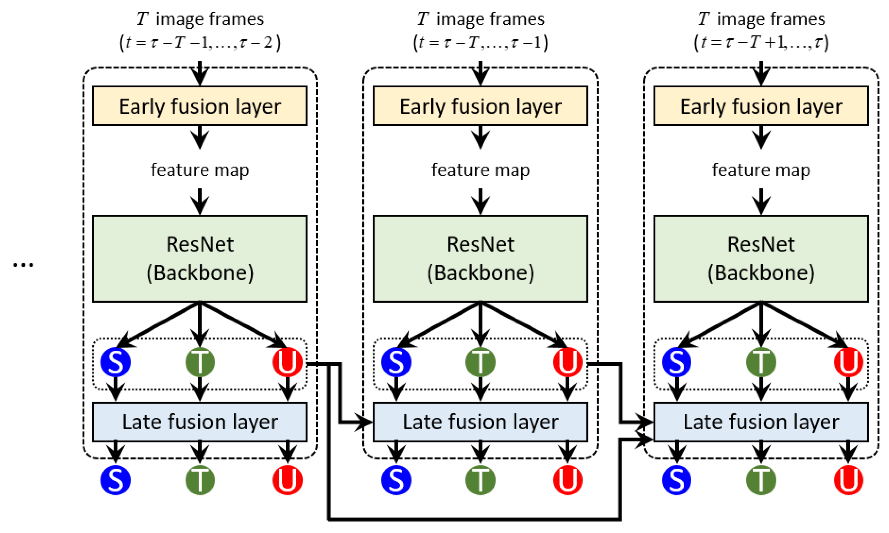
Figure 1.
Proposed model architecture. The colored circles represent probabilities corresponding to three different combustion states: stable, transient, and unstable states colored in blue, green, and red, respectively. Please refer to the text for more detail. Best viewed in color.
Figure 1.
Proposed model architecture. The colored circles represent probabilities corresponding to three different combustion states: stable, transient, and unstable states colored in blue, green, and red, respectively. Please refer to the text for more detail. Best viewed in color.
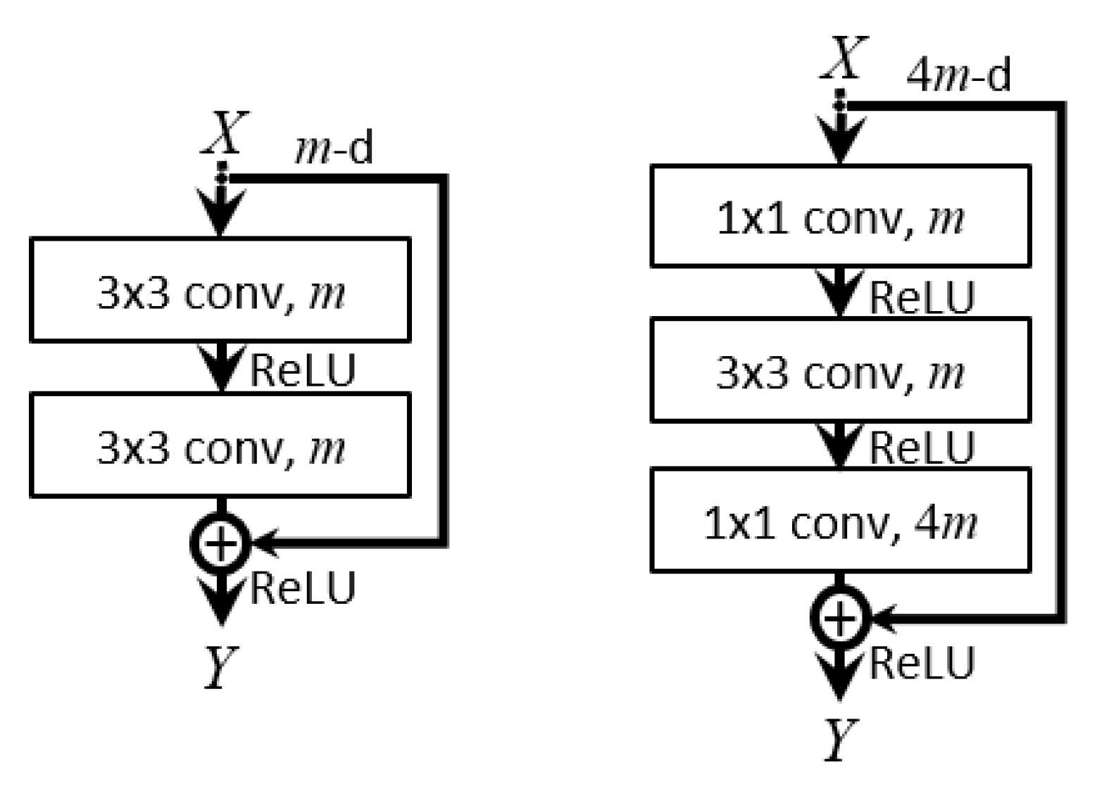
Figure 2.
Examples of convolution blocks with shortcut connections [
24]. (
Left): basic building block for ResNet-18. (
Right): bottleneck building block for ResNet-50.
m and
are the number of filters. We note that every convolution layer is followed by batch normalization.
Figure 2.
Examples of convolution blocks with shortcut connections [
24]. (
Left): basic building block for ResNet-18. (
Right): bottleneck building block for ResNet-50.
m and
are the number of filters. We note that every convolution layer is followed by batch normalization.
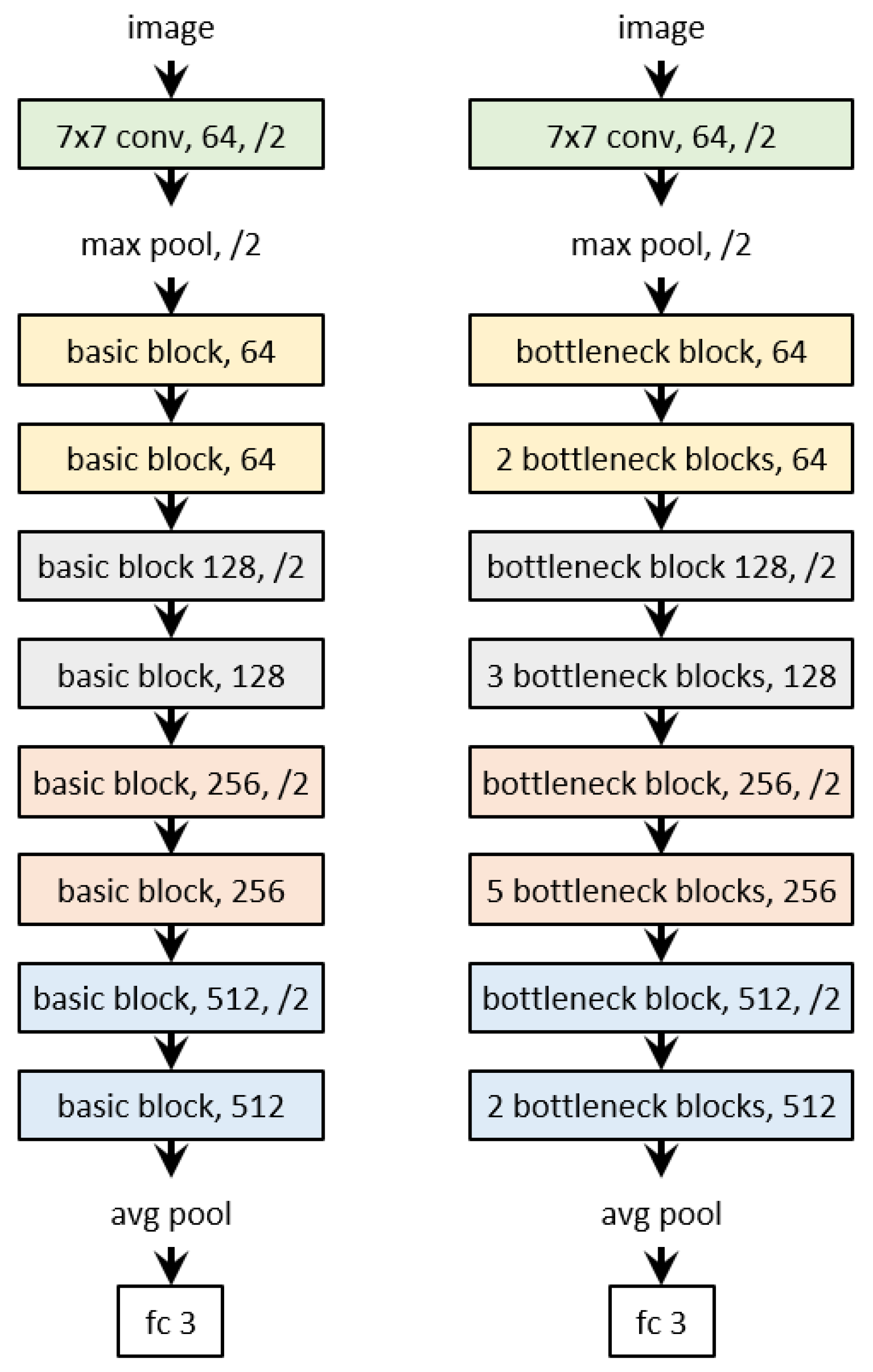
Figure 3.
ResNet-18 and ResNet-50 architectures. (Left): ResNet-18. (Right): ResNet-50. The number to the right of each “block”is the number of filters m. “/2” represents that the feature map height and width are halved by convolution with a stride of 2 or by max-pooling. In every block with “/2”, only the first convolution has a stride of 2. Refer to the text for more detail.
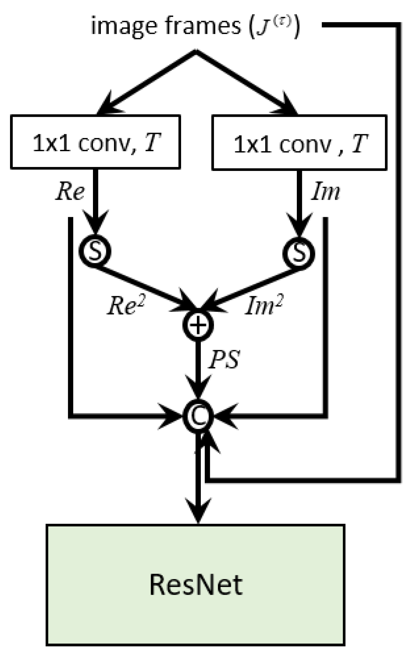
Figure 4.
Our proposed PS-ResNet for early fusion. The two feature maps obtained by convolutions are squared and added together to produce a feature map that can represent the per-pixel power spectral density. The input image sequence and the three feature maps , and are then concatenated to produce the input to a ResNet. In the figure, the “S” circle and the “C” circle represent the square operation and the concatenation operation, respectively. We note that neither batch normalization nor ReLU is applied after the convolutions. Please refer to the text for more detail.
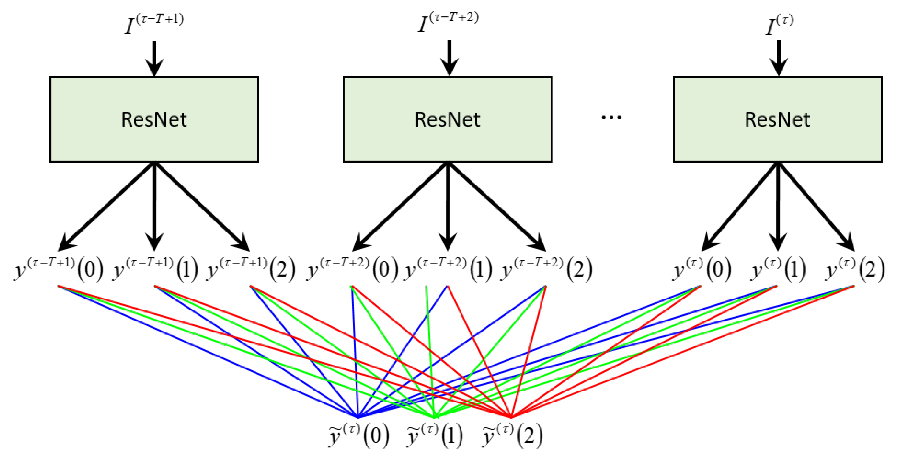
Figure 5.
Our proposed layer for late fusion. The outputs of a ResNet for are concatenated into a -dimensional vector. To obtain the fused output , a fully connected layer is used. The colored lines represent the weights of the fully connected layer. Best viewed in color.
Figure 5.
Our proposed layer for late fusion. The outputs of a ResNet for are concatenated into a -dimensional vector. To obtain the fused output , a fully connected layer is used. The colored lines represent the weights of the fully connected layer. Best viewed in color.
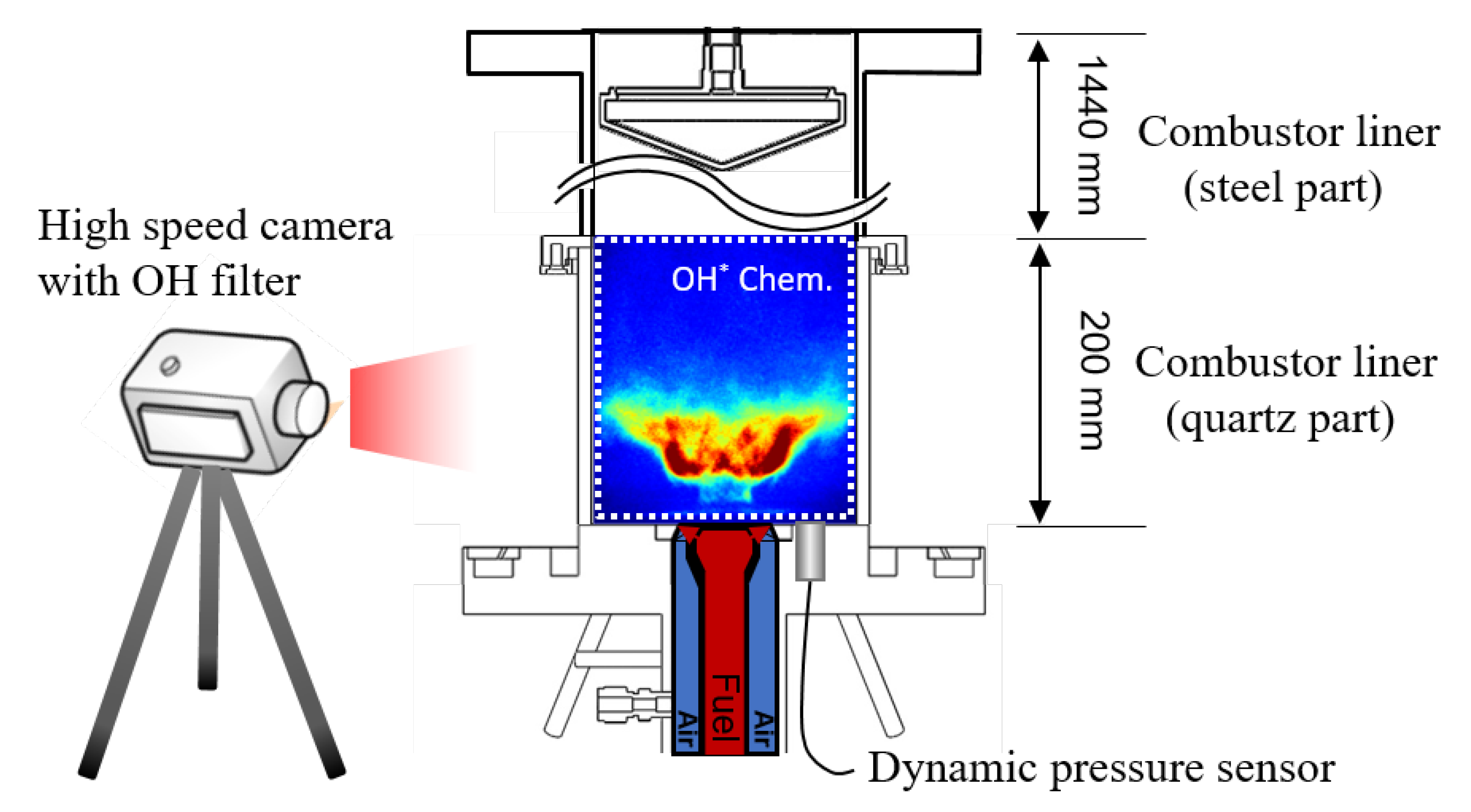
Figure 6.
Schematic of the model gas turbine combustor, dynamic pressure sensor, and HI-CMOS camera position.
Figure 6.
Schematic of the model gas turbine combustor, dynamic pressure sensor, and HI-CMOS camera position.
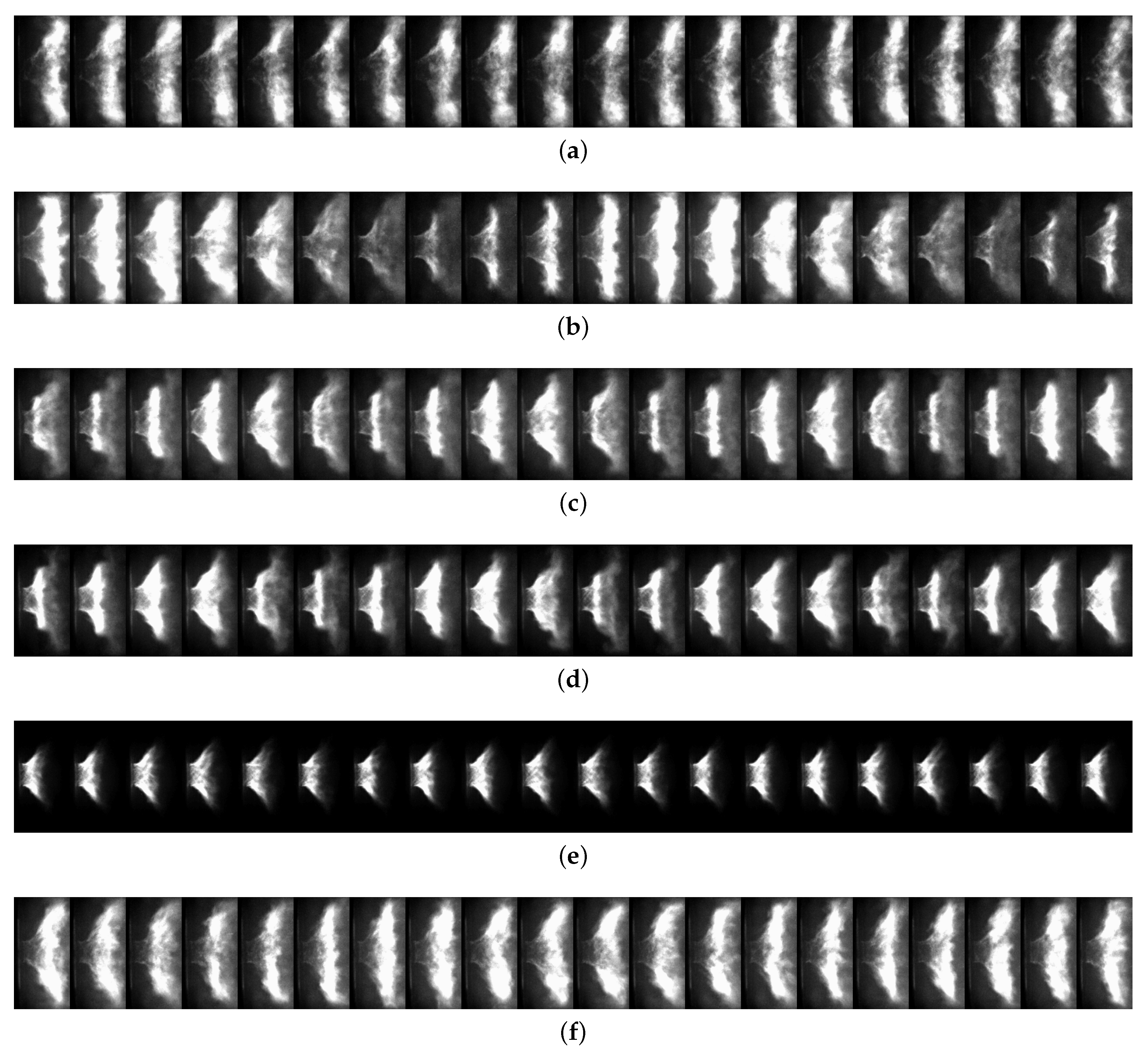
Figure 7.
High-speed flame image sequence dataset. The images have been cropped and brightened for visibility. Below each row of images are shown dynamic pressure (DP), combustion states, and the configuration of training, validation, and test sets. The stable, transient, and unstable states are colored in blue, green, and red, respectively. The black and white boxes represent the validation and test sets, respectively. The remainders are the training sets. Best-viewed in color. (a) Case 1. (b) Case 2. (c) Case 3. (d) Case 4. (e) Case 5. (f) Case 6.
Figure 8.
Approximate fundamental periods of image sequences. Case 1: , Case 2: , Case 3: , Case 4: , Case 5: , Case 6: .
Figure 8.
Approximate fundamental periods of image sequences. Case 1: , Case 2: , Case 3: , Case 4: , Case 5: , Case 6: .
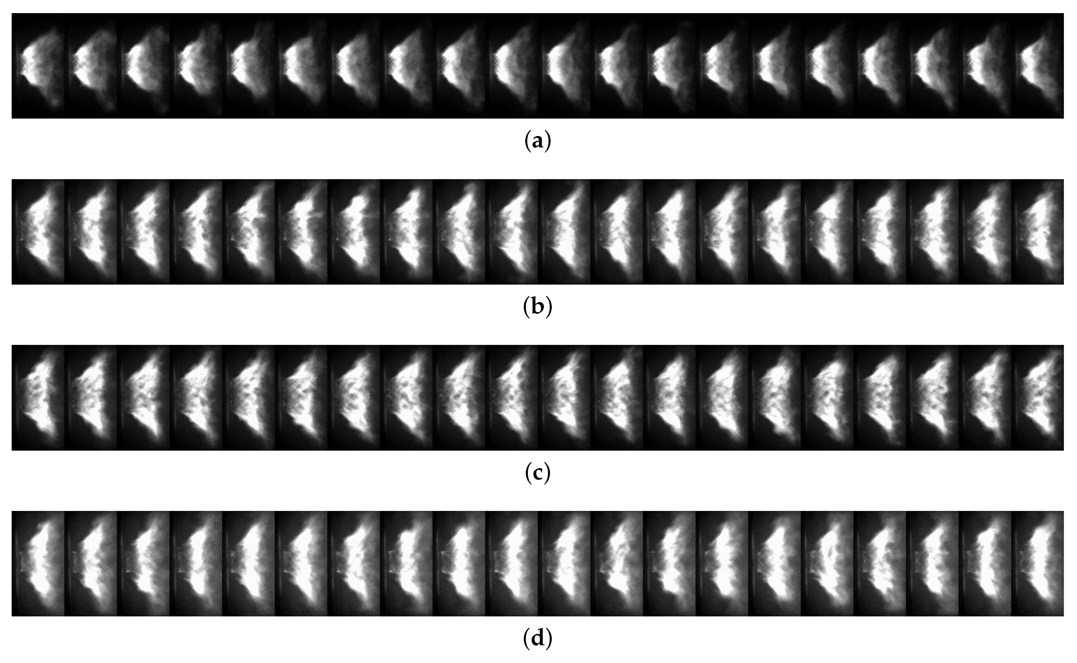
Figure 9.
Subsequent image frames randomly sampled from image sequences. (a) Case 1, . (b) Case 2, t = 38,665, . (c) Case 3, t = 29,204, . (d) Case 4, t = 31,124, . (e) Case 5, t = 10,921, 10,940. (f) Case 6, t = 12,174, .
Figure 9.
Subsequent image frames randomly sampled from image sequences. (a) Case 1, . (b) Case 2, t = 38,665, . (c) Case 3, t = 29,204, . (d) Case 4, t = 31,124, . (e) Case 5, t = 10,921, 10,940. (f) Case 6, t = 12,174, .
Figure 10.
Subsequent image frames randomly sampled from stable and transient sections of Case 3. (a) Case 3, first stable section. (b) Case 3, first transient section. (c) Case 3, second stable section. (d) Case 3, second transient section.
Figure 10.
Subsequent image frames randomly sampled from stable and transient sections of Case 3. (a) Case 3, first stable section. (b) Case 3, first transient section. (c) Case 3, second stable section. (d) Case 3, second transient section.
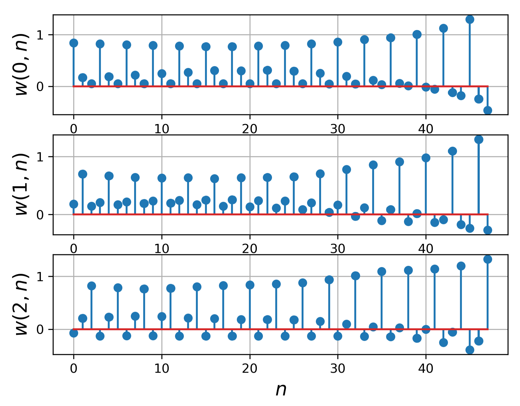
Figure 11.
Learned weights of the proposed late fusion layer for the ResNet-18 with .
Figure 11.
Learned weights of the proposed late fusion layer for the ResNet-18 with .
Table 1.
Experimental conditions for the combustion instability transition.
Table 1.
Experimental conditions for the combustion instability transition.
| Case No. | Initial Fuel Supply Condition | Final Fuel Supply Condition | State Transition |
|---|
| Heat Input (kWth) | H2 (%) | CH4 (%) | Heat Input (kWth) | H2 (%) | CH4 (%) |
|---|
| 1 | 50 | - | 100 | 50 | 12.5 | 87.5 | unstable → stable |
| 2 | 50 | 12.5 | 87.5 | 50 | - | 100 | stable → unstable |
| 3 | 50 | 100 | - | 50 | 75.0 | 25.0 | stable → unstable |
| 4 | 40 | 87.5 | 12.5 | 40 | 75.0 | 25.0 | stable → unstable |
| 5 | 40 | 87.5 | 12.5 | 50 | 87.5 | 12.5 | stable → unstable |
| 6 | 40 | - | 100 | 40 | 12.5 | 87.5 | stable → unstable |
Table 2.
Classification accuracy (%, backbone: ResNet-18).
Table 2.
Classification accuracy (%, backbone: ResNet-18).
| Case No. | | 1 | 2 | 4 | 8 | 16 |
|---|
| 1 | ResNet | 98.0 | 99.0 | 99.0 | 99.5 | 98.9 |
| PS-ResNet | 98.7 | 98.0 | 98.9 | 97.4 | 99.0 |
| 2 | ResNet | 100 | 100 | 100 | 100 | 100 |
| PS-ResNet | 100 | 100 | 100 | 100 | 100 |
| 3 | ResNet | 80.7 | 85.5 | 90.2 | 89.6 | 92.0 |
| PS-ResNet | 86.9 | 87.7 | 87.5 | 84.5 | 93.0 |
| 4 | ResNet | 100 | 100 | 100 | 100 | 100 |
| PS-ResNet | 100 | 100 | 100 | 100 | 100 |
| 5 | ResNet | 96.8 | 98.6 | 99.8 | 100 | 100 |
| PS-ResNet | 97.4 | 98.0 | 99.8 | 100 | 100 |
| 6 | ResNet | 99.8 | 99.8 | 100 | 100 | 100 |
| PS-ResNet | 99.7 | 100 | 100 | 100 | 100 |
| All | ResNet | 95.1 | 96.5 | 97.7 | 97.6 | 98.1 |
| PS-ResNet | 96.6 | 96.8 | 97.1 | 96.2 | 98.3 |
Table 3.
Classification accuracy (%, backbone: ResNet-50).
Table 3.
Classification accuracy (%, backbone: ResNet-50).
| Case No. | | 1 | 2 | 4 | 8 | 16 |
|---|
| 1 | ResNet | 96.1 | 97.5 | 97.6 | 99.2 | 98.8 |
| PS-ResNet | 97.0 | 96.6 | 98.2 | 99.2 | 99.6 |
| 2 | ResNet | 100 | 100 | 100 | 100 | 100 |
| PS-ResNet | 100 | 100 | 100 | 100 | 100 |
| 3 | ResNet | 86.8 | 79.5 | 85.9 | 85.6 | 89.5 |
| PS-ResNet | 88.1 | 83.2 | 86.4 | 87.3 | 88.9 |
| 4 | ResNet | 100 | 100 | 100 | 100 | 100 |
| PS-ResNet | 100 | 100 | 100 | 100 | 100 |
| 5 | ResNet | 97.0 | 98.9 | 99.5 | 99.8 | 100 |
| PS-ResNet | 97.7 | 98.2 | 99.2 | 100 | 100 |
| 6 | ResNet | 99.8 | 100 | 100 | 100 | 100 |
| PS-ResNet | 100 | 100 | 100 | 100 | 100 |
| All | ResNet | 96.3 | 95.0 | 96.5 | 96.7 | 97.5 |
| PS-ResNet | 96.8 | 95.7 | 96.7 | 97.1 | 97.5 |
Table 4.
Confusion matrix (%, ResNet-50, , Case 3).
Table 4.
Confusion matrix (%, ResNet-50, , Case 3).
| Target StatePredicted State | Stable | Transient | Unstable |
|---|
| Stable | 70.5 | 29.6 | 0 |
| Transient | 42.9 | 56.9 | 0.2 |
| Unstable | 0 | 0 | 100 |
Table 5.
Overall classification accuracy (%, backbone: ResNet-18).
Table 5.
Overall classification accuracy (%, backbone: ResNet-18).
| | | 1 | 2 | 4 | 8 | 16 |
|---|
| w.o. late fusion | ResNet | 95.1 | 96.5 | 97.7 | 97.6 | 98.1 |
| PS-ResNet | 96.6 | 96.8 | 97.1 | 96.2 | 98.3 |
| with handcrafted late fusion | ResNet | 95.2 | 96.6 | 98.4 | 98.0 | 98.5 |
| PS-ResNet | 97.7 | 97.9 | 97.5 | 96.5 | 98.6 |
| with learned late fusion | ResNet | 95.2 | 97.0 | 98.4 | 97.6 | 98.1 |
| PS-ResNet | 97.1 | 97.0 | 97.7 | 96.1 | 98.4 |
| with random initialization | ResNet | 95.1 | 97.0 | 98.4 | 97.6 | 98.1 |
| PS-ResNet | 97.0 | 97.1 | 97.7 | 96.1 | 98.5 |
| with RMSprop | ResNet | 95.0 | 97.4 | 98.4 | 97.4 | 97.8 |
| PS-ResNet | 97.1 | 96.8 | 97.5 | 96.5 | 98.3 |
Table 6.
Overall classification accuracy (%, backbone: ResNet-50).
Table 6.
Overall classification accuracy (%, backbone: ResNet-50).
| | | 1 | 2 | 4 | 8 | 16 |
|---|
| w.o. late fusion | ResNet | 96.3 | 95.0 | 96.5 | 96.7 | 97.5 |
| PS-ResNet | 96.8 | 95.7 | 96.7 | 97.1 | 97.5 |
| with handcrafted late fusion | ResNet | 97.1 | 95.2 | 97.0 | 96.7 | 97.9 |
| PS-ResNet | 98.0 | 96.2 | 97.0 | 97.5 | 98.0 |
| with learned late fusion | ResNet | 96.9 | 95.2 | 96.7 | 96.7 | 97.7 |
| PS-ResNet | 98.0 | 95.5 | 96.3 | 97.2 | 97.4 |
| with random initialization | ResNet | 96.9 | 95.2 | 96.9 | 96.8 | 97.8 |
| PS-ResNet | 97.8 | 95.9 | 96.3 | 97.4 | 97.4 |
| with RMSprop | ResNet | 96.9 | 95.4 | 96.5 | 96.4 | 97.7 |
| PS-ResNet | 97.6 | 96.3 | 96.6 | 97.3 | 97.4 |
Table 7.
Average processing time per time step.
Table 7.
Average processing time per time step.
| Backbone | | Early Fusion | Late Fusion | Time (ms) |
|---|
| ResNet-18 | 1 | no | no | 5.21 |
| yes | no | 5.50 |
| yes | yes | 7.88 |
| 16 | no | no | 7.18 |
| yes | no | 8.33 |
| yes | yes | 8.44 |
| ResNet-50 | 1 | no | no | 10.06 |
| yes | no | 10.09 |
| yes | yes | 11.88 |
| 16 | no | no | 11.49 |
| yes | no | 11.80 |
| yes | yes | 12.17 |


