A Robust Structured Tracker Using Local Deep Features

Abstract

Deep features extracted from convolutional neural networks have been recently utilized in visual tracking to obtain a generic and semantic representation of target candidates. In this paper, we propose a robust structured tracker using local deep features (STLDF). This tracker exploits the deep features of local patches inside target candidates and sparsely represents them by a set of templates in the particle filter framework. The proposed STLDF utilizes a new optimization model, which employs a group-sparsity regularization term to adopt local and spatial information of the target candidates and attain the spatial layout structure among them. To solve the optimization model, we propose an efficient and fast numerical algorithm that consists of two subproblems with the close-form solutions. Different evaluations in terms of success and precision on the benchmarks of challenging image sequences (e.g., OTB50 and OTB100) demonstrate the superior performance of the STLDF against several state-of-the-art trackers.

1. Introduction

Visual tracking aims to estimate states of a moving object or multiple objects in frame sequences under different conditions. It has been considered as one of the most active and challenging computer vision topics with a large array of applications in autonomous driving, video content analysis and understanding, surveillance, and so forth. Although some improvements have been achieved in several tracking methods [1,2,3,4,5,6], computer vision researchers still aim to develop more robust algorithms capable of handling various challenges including occlusion, illumination variations, in-plane and out-plane rotation, background clutter, deformation, and low resolution.

In general, visual tracking algorithms can be categorized into two groups: discriminative and generative. Discriminative tracking methods formulate a binary decision boundary to distinguish the target from backgrounds. Ensemble [7], online boosting [8], and online multiple instance learning [9] are a few representative discriminative methods. Generative methods adopt a model to represent the target and formulate tracking as a model-based searching procedure to find the most similar region to the target. Eigenspace learning [10], incremental subspace learning [11], and sparse representation [5,12,13,14] are a few representative generative methods. The performance of these approaches is limited due to the use of hand-crafted features such as intensity, local binary pattern (LBP) [15], and histogram of oriented gradient (HOG) [16] for target representation. These features may not be effective to handle immense challenges imposed on various frame sequences.

Convolutional neural networks (CNNs) have been applied recently to visual tracking with tremendous improvement [17,18,19,20,21,22,23]. As one of the pioneer works, Wang and Yeung [17] propose a multi-layer denoising auto-encoder network to learn general object representations that are more robust against variations for visual tracking. Later, Wang et al. [24] use auxiliary video sequences to learn hierarchical features, which are robust to both complicated motion transformations and appearance changes of target objects. This feature learning algorithm is further integrated into three tracking methods to achieve significant improvement. Several recent tracking algorithms [25,26] utilize pretrained CNNs on a large-scale classification dataset (e.g., ImageNet [27]) to extract hierarchical features. These features are then separately integrated in correlation filter-based trackers and sparse trackers [19,20,23] to achieve better tracking performance than using hand-crafted features. On the other hand, some deep learning-based tracking methods [28,29] directly use external videos to train CNNs for visual tracking. Nam and Han [28] introduce the MDNet tracker to pretrain a discriminative CNN using auxiliary sequences with tracking ground truths to obtain a generic object representation. Since then, various trackers have been proposed to improve the performance of MDNet by using a tree structure to manage multiple target appearance models [30], using adversarial learning to identify a mask that maintains the most robust features of the target objects over a long temporal span [31], and using reciprocative learning to exploit visual attention for training deep classifiers [32]. All these direct CNN-based trackers achieve improved performance. However, they all require off-line training on the external videos.

In this paper, we propose a robust structured tracker using local deep features (STLDF), which exploits the convolutional neural networks (CNNs) features of the local patches inside a target candidate and sparsely represents them in a novel convex optimization model. Unlike the conventional local sparse trackers [14], the proposed optimization model in STLDF employs a group-sparsity regularization term to adopt local and spatial information of the target candidates and attain the spatial layout structure among them. The major contributions of the proposed work are summarized as follows:

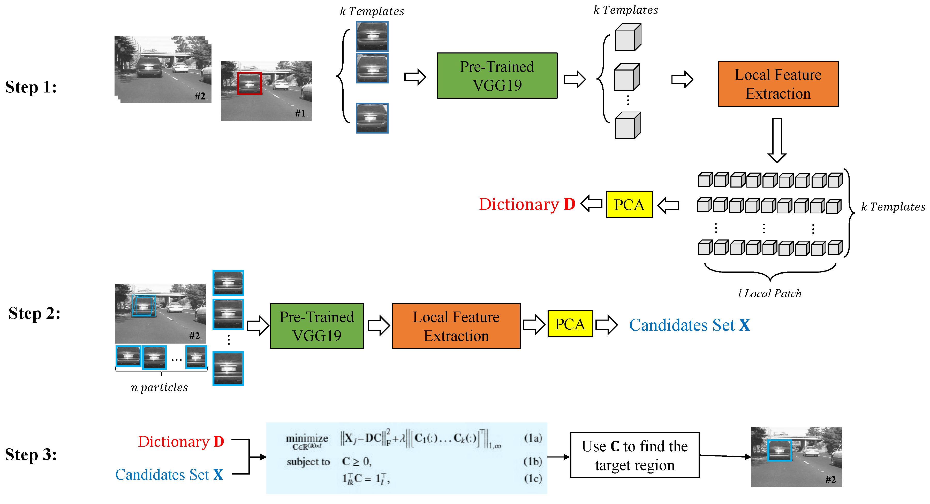
• Proposing a deep features-based structured local sparse tracker, which employs CNN deep features of the local patches within a target candidate and keeps the relative spatial structure among the local deep features of a target candidate.
• Developing a convex optimization model, which combines nine local features of each target candidate with a group-sparsity regularization term to encourage the tracker to sparsely select appropriate local patches of the same subset of templates.
• Designing a fast and parallel numerical algorithm by deriving the augmented Lagrangian of the optimization model into two close-form problems: the quadratic problem and the Euclidean norm projection onto probability simplex constraints problem by adopting the alternating direction method of multiplier (ADMM).
• Utilizing the accelerated proximal gradient (APG) method to update the CNN deep feature-based template by casting it as a Lasso problem.

The preliminary results of this work are presented in Reference [33], which is based on hand-crafted features. We made a number of improvements in the proposed method: (i) STLDF automatically extracts representative local deep features of target candidates using the pre-trained CNN. (ii) STLDF efficiently derives the augmented Lagrangian of the optimization model into two close-form problems: the quadratic problem and the Euclidean norm projection onto probability simplex constraints problem. (iii) STLDF updates the CNN deep feature-based template by casting it as a Lasso problem and numerically solving it using the accelerated proximal gradient (APG) method. The remainder of this paper is organized as follows: Section 2 introduces the notations used in the paper. Section 3 presents the STLDF together with its new convex optimization model solved by the proposed ADMM-based numerical solution. In addition, this section explains the deep feature extraction, the template updates strategies, and the summary of the proposed method. Section 4 demonstrates the experimental results on OTB50 and OTB100 challenging tracking benchmarks, quantitatively and qualitatively compares the STLDF with several state-of-the-art trackers, and discusses the results and future work. Section 5 draws the conclusions and presents the future work.

2. Notations

In this paper, we denote scalars, vectors, and matrices by italic lowercase, boldface lowercase, and boldface uppercase letters, respectively. For a column vector $\mathbf{x}$, we use ${\mathbf{x}}_i$ to represent the ith element of $\mathbf{x}$ and $\mathrm{diag}\left(\mathbf{x}\right)$ to represent a diagonal matrix formed by the elements of $\mathbf{x}$. For a matrix $\mathbf{X}$, we use ${\mathbf{X}}_{i,j}$ to denote the element at the ith row and jth column, ${∥\mathbf{X}∥}_{\mathrm{F}}$ to denote the Frobenious norm, and ${∥\mathbf{X}∥}_{p,q}$ to denote the ${\ell }_p$ norm of ${\ell }_q$ norm of the rows in $\mathbf{X}$. In addition, we use $\mathrm{tr}(·)$ as the trace operator, $\mathbf{X}\otimes \mathbf{Y}$ as the Kronecker product on two matrices $\mathbf{X}$ and $\mathbf{Y}$, ${\mathbf{1}}_l$ as a column vector of all ones, and ${\mathbf{I}}_k$ as a $k\times k$ identity matrix.

3. Proposed Method

In this section, we present the proposed structured tracker using local deep features (STLDF). In Section 3.1, we formulate a convex optimization model, which incorporates the local deep features of target candidates to overcome the drawbacks of traditional local sparse trackers [14,34]. In Section 3.2, we describe a numerical algorithm in detail, which efficiently solves the optimization model presented in Section 3.1. In Section 3.3, we present the local deep feature extraction process using a pre-trained CNN. In Section 3.4, we describe the template update strategy. In Section 3.5, we provide a summary of the proposed STLDF tracker.

3.1. Structured Tracker Using Local Deep Features (STLDF)

The proposed STLDF tracker incorporates the local deep features of target candidates in a new optimization model to achieve robust tracking performance. Unlike traditional local sparse trackers, this convex optimization model encourages the tracker to keep the spatial layout structure among different local deep features of a target candidate. As a result, it achieves a consistent and similar pattern on the non-zero elements of the sparse vectors corresponding to different local deep features.

Traditional local sparse trackers [14,34] do not attain the spatial layout structure among local patches. For instance, Jia et al. [34] use the Lasso model to represent local patches of target candidates. However, the ${\ell }_1$ regularization term in Lasso does not encourage the tracker to represent local patches inside a target candidate by their corresponding local patches of select dictionary bases. The proposed STLDF tracker employs a new optimization model to address the above issue related to conventional local sparse trackers [14,34]. Specifically, the group sparsity regularization term in the optimization model of STLDF imposes a structure on the sparse vectors of different local patches inside each target candidate. This regularization term selects few templates for representation and motivates the group of local patches inside a target candidate to be represented by a group of local patches inside the few template sets. For instance, if the rth local patch of the jth target candidate is best represented by the rth local patch of the qth template, the sth local patch of the jth target candidate is also best represented by the sth local patch of the qth template. To solve the optimization model, we adopt alternating direction method of multiplier (ADMM) to convert the augmented Lagrangian of the optimization model into two suproblems with close-form solutions: the quadratic problem and the Euclidean norm projection onto probability simplex constraints problem.

We select l overlapping local patches in k target templates and extract a d-dimensional feature vector for each patch. These feature vectors are used to build the dictionary $\mathbf{D}=[{\mathbf{D}}_1,\dots ,{\mathbf{D}}_k]\in {\mathbb{R}}^{d\times \left(lk\right)}$, where ${\mathbf{D}}_i\in {\mathbb{R}}^{d\times l}$. Using n number of particles (target candidates), we build a matrix $\mathbf{X}=[{\mathbf{X}}_1,\dots ,{\mathbf{X}}_n]\in {\mathbb{R}}^{d\times \left(ln\right)}$ to include local deep features of target candidates. We denote the sparse coefficient matrix as $\mathbf{C}\triangleq {\left[\begin{array}{ccc}{\mathbf{C}}_1& \dots & {\mathbf{C}}_k\end{array}\right]}^{\top }\in {\mathbb{R}}^{\left(lk\right)\times l}$, where ${\left\{{\mathbf{C}}_q\right\}}_{q=1}^k$ is a $l\times l$ matrix indicating the group representation of l local features of the jth target candidate using l local features of the qth template. We formulate the following model to represent deep features of the jth target candidate using k target templates:

$$\begin{array}{c}\underset{\mathbf{C}\in {\mathbb{R}}^{\left(lk\right)\times l}}{\mathrm{minimize}}\hspace{1em}{\Vert {\mathbf{X}}_j-\mathbf{DC}\Vert }_{\mathrm{F}}^2+\lambda {\Vert {\left[{\mathbf{C}}_1\right(:)\dots {\mathbf{C}}_k(:\left)\right]}^{\top }\Vert }_{1,\infty }\end{array}$$

(1a)

$$\begin{array}{c}\mathrm{subject}\mathrm{to}\hspace{1em}\mathbf{C}\ge 0,\end{array}$$

(1b)

$${\mathbf{1}}_{lk}^{\top }\mathbf{C}={\mathbf{1}}_l^{\top },$$

(1c)

The first term in (1a) represents the similarity measurement between the feature matrix ${\mathbf{X}}_j$ and its representation using the dictionary $\mathbf{D}$. The second term is a group-sparsity regularization term, which is a penalization term in the objective function to select dictionary words (templates). This term also establishes the ${∥·∥}_{1,\infty }$ minimization on matrix ${\left[\begin{array}{c}{\mathbf{C}}_1(:)\dots {\mathbf{C}}_k(:)\end{array}\right]}^{\top }$, which leads to imposing local features inside a target candidate to choose similar few dictionary words (templates). It should be noted that each group (${\mathbf{C}}_q$ of $l\times l$) is vectorized via ${\mathbf{C}}_q(:)$ and is represented by a column vector. The sum of the maximum absolute values per group is minimized by imposing ${∥·∥}_{1,\infty }$. Therefore, the $l_1$ norm minimization selects few dictionary words for representation by imposing the rows of ${\left[\begin{array}{c}{\mathbf{C}}_1(:)\dots {\mathbf{C}}_k(:)\end{array}\right]}^{\top }$ to be sparse. The $l_{\infty }$ norm minimization on the columns of ${\left[\begin{array}{c}{\mathbf{C}}_1(:)\dots {\mathbf{C}}_k(:)\end{array}\right]}^{\top }$ motivates the group of local patches to jointly select similar few templates. The parameter $\lambda >0$ is a trade-off between the first and the second terms. The constraint (1b) ensures sparse coefficients to be non-negative since a tracking target can be represented by target templates dominated by non-negative coefficients [12]. The constraint (1c) ensures that each local feature vector in ${\mathbf{X}}_j$ is expressed by at least one selected local feature vector of the dictionary $\mathbf{D}$.

In order to find the representation of each target candidate, we compute the matrix $\mathbf{C}$ using the numerical algorithm introduced in Section 3.2. By applying average pooling on $\mathbf{C}$, we obtain a representative vector for each target candidate [34]. The summation of this representative vector is used as a likelihood value to determine the best target candidate among n target candidates in each frame. The templates are updated to maintain the latest changes of target regions over time [34].

3.2. Numerical Algorithm

In this section, we provide a fast and parallel numerical algorithm by deriving the augmented Lagrangian of the optimization model (1) into two close-form problems based on the alternating direction method of multipliers (ADMM) [35]. In general, ADMM incorporates supplementary variables to model a complex optimization problem to simpler sub-problems. Each sub-problem is iteratively solved using an explicit solution till it converges. To do so, we first define vector $\mathbf{m}\in {\mathbb{R}}^k$ such that ${\mathbf{m}}_i=\arg \max |{\mathbf{C}}_i(:)|$ and rewrite (1) as:

$$\begin{array}{c}\underset{\underset{\mathbf{m}\in {\mathbb{R}}^k}{\mathbf{C}\in {\mathbb{R}}^{\left(lk\right)\times l}}}{\mathrm{minimize}}\hspace{1em}{\Vert {\mathbf{X}}_j-\mathbf{DC}\Vert }_{\mathrm{F}}^2+\lambda {\mathbf{1}}_k^{\top }\mathbf{m}\end{array}$$

(2a)

$$\begin{array}{c}\mathrm{subject}\mathrm{to}\hspace{1em}\mathbf{C}\ge 0,\end{array}$$

(2b)

$${\mathbf{1}}_{\left(lk\right)}^{\top }\mathbf{C}={\mathbf{1}}_l^{\top },$$

(2c)

$$\mathbf{m}\otimes {\mathbf{1}}_l{\mathbf{1}}_l^{\top }\ge \mathbf{C}.$$

(2d)

To ensure the equivalency between (1) and (2), we impose the inequality constraint (2d). To simplify our model, we convert this inequality constraint to an equality one (2) by introducing a non-negative slack matrix $\mathbf{U}\in {\mathbb{R}}^{\left(lk\right)\times l}$ to compensate the difference between $\mathbf{m}\otimes {\mathbf{1}}_l{\mathbf{1}}_l^{\top }$ and $\mathbf{C}$. Therefore, we rewrite (2) as:

$$\begin{array}{c}\underset{\underset{\mathbf{m}\in {\mathbb{R}}^k}{\mathbf{C},\mathbf{U}\in {\mathbb{R}}^{\left(lk\right)\times l}}}{\mathrm{minimize}}\hspace{1em}{\Vert {\mathbf{X}}_j-\mathbf{DC}\Vert }_{\mathrm{F}}^2+\lambda {\mathbf{1}}_k^{\top }\mathbf{m}\end{array}$$

(3a)

$$\begin{array}{c}\mathrm{subject}\mathrm{to}\hspace{1em}\mathbf{C}\ge 0,\end{array}$$

(3b)

$${\mathbf{1}}_{\left(lk\right)}^{\top }\mathbf{C}={\mathbf{1}}_l^{\top },$$

(3c)

$$\mathbf{m}\otimes {\mathbf{1}}_l{\mathbf{1}}_l^{\top }=\mathbf{C}+\mathbf{U},$$

(3d)

$$\mathbf{U}\ge 0.$$

(3e)

We rewrite the inequality constraint (3d) independent of $\mathbf{m}$ in (4d) since this inequality suggests that the columns of $\mathbf{C}+\mathbf{U}$ are regulated to be identical. In addition, we rewrite ${\mathbf{1}}_k^{\top }\mathbf{m}$ as $\frac{1}{l^2}{\mathbf{1}}_{\left(lk\right)}^{\top }(\mathbf{C}+\mathbf{U}){\mathbf{1}}_l$ using (3d). These make (3) be independent of $\mathbf{m}$ as:

$$\begin{array}{c}\underset{\mathbf{C},\mathbf{U}\in {\mathbb{R}}^{\left(lk\right)\times l}}{\mathrm{minimize}}\hspace{1em}{\Vert {\mathbf{X}}_j-\mathbf{DC}\Vert }_{\mathrm{F}}^2+\frac{\lambda }{l^2}{\mathbf{1}}_{\left(lk\right)}^{\top }(\mathbf{C}+\mathbf{U}){\mathbf{1}}_l\end{array}$$

(4a)

$$\mathrm{subject}\mathrm{to}\hspace{1em}\mathbf{C}\ge 0,$$

(4b)

$${\mathbf{1}}_{\left(lk\right)}^{\top }\mathbf{C}={\mathbf{1}}_l^{\top },$$

(4c)

$$\mathbf{E}(\mathbf{C}+\mathbf{U})=\frac{{\mathbf{I}}_k\otimes {\mathbf{1}}_l{\mathbf{1}}_l^{\top }}{l}(\mathbf{C}+\mathbf{U}),$$

(4d)

$$\mathbf{U}\ge 0,$$

(4e)

where matrix $\mathbf{E}$ is the right circular shift operator on the rows of $\mathbf{C}+\mathbf{U}$. Based on ADMM, we define $\widehat{\mathbf{C}},\widehat{\mathbf{U}}\in {\mathbb{R}}^{\left(lk\right)\times l}$ as supplementary variables and reformulate (4) as:

$$\begin{array}{c}\underset{\mathbf{C},\widehat{\mathbf{C}},\mathbf{U},\widehat{\mathbf{U}}\in {\mathbb{R}}^{\left(lk\right)\times l}}{\mathrm{minimize}}\hspace{1em}{\Vert {\mathbf{X}}_j-\mathbf{DC}\Vert }_{\mathrm{F}}^2+\frac{\lambda }{l^2}{\mathbf{1}}_{\left(lk\right)}^{\top }(\mathbf{C}+\mathbf{U}){\mathbf{1}}_l+\frac{{\mu }_1}{2}\Vert \mathbf{C}-\widehat{\mathbf{C}}{\Vert }_{\mathrm{F}}^2+\frac{{\mu }_2}{2}\Vert \mathbf{U}-\widehat{\mathbf{U}}{\Vert }_{\mathrm{F}}^2\end{array}$$

(5a)

$$\mathrm{subject}\mathrm{to}\hspace{1em}\widehat{\mathbf{C}}\ge 0,$$

(5b)

$${\mathbf{1}}_{\left(lk\right)}^{\top }\widehat{\mathbf{C}}={\mathbf{1}}_l^{\top },$$

(5c)

$$\mathbf{E}(\mathbf{C}+\mathbf{U})=\frac{{\mathbf{I}}_k\otimes {\mathbf{1}}_l{\mathbf{1}}_l^{\top }}{l}(\mathbf{C}+\mathbf{U}),$$

(5d)

$$\widehat{\mathbf{U}}\ge 0,$$

(5e)

$$\mathbf{C}=\widehat{\mathbf{C}},\hspace{1em}\mathbf{U}=\widehat{\mathbf{U}}.$$

(5f)

where ${\mu }_1,{\mu }_2>0$ are the augmented Lagrangian parameters. Without loss of generality, we assume these parameters are the same [35]. For any feasible solution of (5a), the last two terms are equal to zero, which implies the equivalency between (4) and (5). The augmented Lagrangian function of (5) is as follows:

$$\begin{array}{cc}{\mathcal{L}}_{\mu }(\mathbf{C},\mathbf{U},\widehat{\mathbf{C}},\widehat{\mathbf{U}},{\mathsf{\Lambda }}_1,{\mathsf{\Lambda }}_2)=\hfill & {∥{\mathbf{X}}_j-\mathbf{D}\mathbf{C}∥}_{\mathrm{F}}^2+\frac{\lambda }{l^2}{\mathbf{1}}_{\left(lk\right)}^{\top }(\mathbf{C}+\mathbf{U}){\mathbf{1}}_l\hfill \\ & +\frac{\mu }{2}{∥\mathbf{C}-\widehat{\mathbf{C}}+\frac{{\mathsf{\Lambda }}_1}{\mu }∥}_{\mathrm{F}}^2+\frac{\mu }{2}{∥\mathbf{U}-\widehat{\mathbf{U}}+\frac{{\mathsf{\Lambda }}_2}{\mu }∥}_{\mathrm{F}}^2,\hfill \end{array}$$

(6)

where ${\mathsf{\Lambda }}_1,{\mathsf{\Lambda }}_2\in {\mathbb{R}}^{\left(lk\right)\times l}$ are the Lagrangian multipliers corresponding to the equations in (5f). Given initialization for $\widehat{\mathbf{C}}$, $\widehat{\mathbf{U}}$, ${\mathsf{\Lambda }}_1$, and ${\mathsf{\Lambda }}_2$ at time $t=0$ (e.g., ${\widehat{\mathbf{C}}}^0,{\widehat{\mathbf{U}}}^0,{\mathsf{\Lambda }}_1^0,{\mathsf{\Lambda }}_2^0$), (6) is solved through the ADMM iterations described below:

$$\begin{array}{c}({\mathbf{C}}^{t+1},{\mathbf{U}}^{t+1}):=\underset{\mathbf{C},\mathbf{U}\in {\mathbb{R}}^{\left(lk\right)\times l}}{\arg \min }\hspace{1em}{\mathcal{L}}_{\mu }(\mathbf{C},\mathbf{U},{\widehat{\mathbf{C}}}^t,{\widehat{\mathbf{U}}}^t,{\mathsf{\Lambda }}_1^t,{\mathsf{\Lambda }}_2^t)\\ \mathrm{subject}\mathrm{to}\left(5\mathrm{d}\right)\end{array}$$

(7)

$$\begin{array}{c}({\widehat{\mathbf{C}}}^{t+1},{\widehat{\mathbf{U}}}^{t+1}):=\underset{\mathbf{C},\mathbf{U}\in {\mathbb{R}}^{\left(lk\right)\times l}}{\arg \min }\hspace{0.17em}{\mathcal{L}}_{\mu }({\mathbf{C}}^{t+1},{\mathbf{U}}^{t+1},\widehat{\mathbf{C}},\widehat{\mathbf{U}},{\mathsf{\Lambda }}_1^t,{\mathsf{\Lambda }}_2^t)\\ \mathrm{subject}\mathrm{to}\left(5\mathrm{b}\right),\left(5\mathrm{c}\right),\left(5\mathrm{e}\right).\end{array}$$

(8)

$$\begin{array}{cc}\hfill & {\mathsf{\Lambda }}_1^{t+1}={\mathsf{\Lambda }}_1^t+\mu ({\mathbf{C}}^{t+1}-{\widehat{\mathbf{C}}}^{t+1})\hfill \\ \hfill & {\mathsf{\Lambda }}_2^{t+1}={\mathsf{\Lambda }}_2^t+\mu ({\mathbf{U}}^{t+1}-{\widehat{\mathbf{U}}}^{t+1})\hfill \end{array}.$$

(9)

By considering the quadratic and linear terms of $\mathbf{C}$ and $\mathbf{U}$ in (6), we first define ${\left\{{\mathbf{z}}_i\right\}}_{i=1}^{lk}$, where ${\mathbf{z}}_i\in {\mathbb{R}}^{2l}$ is obtained by stacking the ith rows of $\mathbf{C}$ and $\mathbf{U}$. We then divide (7) into $lk$ equality constrained quadratic programs as follows:

$$\begin{array}{c}\underset{{\mathbf{z}}_i\in {\mathbb{R}}^{2l}}{\mathrm{minimize}}\hspace{1em}\frac{1}{2}{{\mathbf{z}}_i}^{\top }{\mathbf{Q}}_{\mathbf{Z}i}+{{\mathbf{z}}_i}^{\top }{\mathbf{q}}_i\end{array}$$

(10a)

$$\mathrm{subject}\mathrm{to}\hspace{1em}\mathbf{A}{\mathbf{z}}_i=0,$$

(10b)

where $\mathbf{Q}\in {\mathbb{R}}^{l\times l}$ is a block diagonal positive semi-definite matrix and $\mathbf{A}$ is a sparse matrix constructed based on the constraint (5d). Each of the above quadratic programs has its analytical solution by writing the KKT conditions.

Similarly, we split (8) into two separate sub-problems with close-form solutions over $\widehat{\mathbf{C}}$ and $\widehat{\mathbf{U}}$ as follows:

$$\begin{array}{c}\underset{{\mathbf{z}}_i\in {\mathbb{R}}^{2l}}{\mathrm{minimize}}\hspace{1em}\Vert \widehat{\mathbf{C}}-(\mathbf{C}+\frac{{\mathbf{\Lambda }}_1}{\mu }){\Vert }_{\mathrm{F}}^2\end{array}$$

(11a)

$$\mathrm{subject}\mathrm{to}\hspace{1em}\widehat{\mathbf{C}}\ge 0,$$

(11b)

$${\mathbf{1}}_{\left(lk\right)}^{\top }\widehat{\mathbf{C}}={\mathbf{1}}_l^{\top },$$

(11c)

$$\begin{array}{c}\underset{{\mathbf{z}}_i\in {\mathbb{R}}^{2l}}{\mathrm{minimize}}\hspace{1em}\Vert \widehat{\mathbf{U}}-(\mathbf{U}+\frac{{\mathbf{\Lambda }}_2}{\mu }){\Vert }_{\mathrm{F}}^2\end{array}$$

(12a)

$$\mathrm{subject}\mathrm{to}\hspace{1em}\widehat{\mathbf{U}}\ge 0,$$

(12b)

where sub-problems (11) and (12) consist of l independent Euclidean norm projections onto the probability simplex constraints and the non-negative orthant, respectively. Both sub-problems have analytical solutions. Finally, we solve the two sub-problems over ${\mathsf{\Lambda }}_1$ and ${\mathsf{\Lambda }}_2$ in (9) by performing l parallel updates over their respective columns. The closed form solutions lead to quick updates in each iteration.

3.3. Local Deep Feature Extraction

In the proposed STLDF, we automatically extract learned local deep features to represent each target region. To this end, we set the size of each target candidate to $64\times 64$ pixels to contain sufficient object-level information with decent resolution. Each target candidate is passed to the pre-trained VGG19 [27] network on the large-scale ImageNet dataset [36] to automatically extract their representative features. This network has been proven to achieve better tracking performance than other CNNs such as AlexNet since its strengthened semantic with deeper architecture is more insensitive to significant appearance change. Its default input size of $224\times 224\times 3$ has also been used in other VGG19-based trackers [23,37] to achieve good tracking results. To ensure fair comparison with other VGG19-based trackers, we resize each target candidate to this default input size before forward propagation. We utilize the output of the Conv5-4 layer as the feature map of the target candidate since the fifth layer is proven to be effective in discriminating the targets even with dramatic background changes [37]. The generated feature map has a size of $7\times 7\times 512$, which is not large enough to provide spatial information of target candidates. As a result, we use the bilinear interpolation technique introduced in Reference [37] to perform a two-layer upsampling operation to increase the feature map from $7\times 7\times 512$ to $14\times 14\times 512$ then to $28\times 28\times 512$. The final upsampled feature map is of sufficient spatial resolution to extract overlapping local patches of size $14\times 14\times 512$, which has been shown to be effective in discriminating the target [37], to provide more detailed local information. To this end, we employ the concept of shared features [38] to extract l local deep features inside the upsampled feature map. To do so, we divide the upsampled feature map into $l=9$ overlapping $14\times 14\times 512$ features maps with the stride of 7. The feature map of each of 9 overlapping patches is vectorized as a feature vector with the size of $1\times 100352$. Finally, we apply principal component analysis (PCA) on the feature vector of each patch to attain the top 1120 principal components for each local feature vector (e.g., $d=1120$) to speed up the process to find the best target candidate by the proposed optimization model. We choose 1120 principal components since at least 95% of variance is retained.

3.4. Template Update

We adopt the same strategy as that used in Reference [34] to update templates. We generate a cumulative probability sequence and a random number according to uniform distribution on the unit interval $[0,1]$. We then choose the template to be replaced based on the section that the random number lies in. This ensures that the old templates are slowly updated and the new ones are quickly updated. As a result, the drifting issues are alleviated.

We replace the selected template by using the information of the tracking result in the current frame. To do so, we represent the tracking result by a dictionary in a Lasso problem. This dictionary contains trivial templates (identity matrix) [12] and PCA basis vectors, which are calculated from the templates $\mathbf{D}$. We numerically solve the Lasso problem using the accelerated proximal gradient (APG) method. To further improve the computational time, we consider the structure of the identity matrix in our Lasso numerical solver to quickly perform the matrix multiplications and find the descend direction faster in each iteration.

3.5. STLDF Summary

The tracking steps of the proposed STLDF for two consecutive frames (i.e., frame #1 and frame #2) are summarized in Figure 1. In the first step, local deep features of k target templates are extracted using the initial target location in the frame #1. Their top principal components are selected using PCA. The dictionary $\mathbf{D}$ consisting of these local deep features is then constructed. The interested readers may refer to Section 3.1 and Section 3.3 for details. In the second step, local deep features of target candidates are extracted to construct $\mathbf{X}$ in the frame #2. In the third step, local deep features of each target candidate, ${\mathbf{X}}_j$, is represented by the dictionary matrix in the optimization model in (1). Finally, the optimization model is iteratively solved to obtain $\mathbf{C}$ for each target candidate using (7), (8), and (9). The best target candidate with the minimum reconstruction error is then selected as the target candidate. The tracking continues for the next frame using the previously estimated target location and templates are updated as explained in Section 3.4 until all the frames are processed.

4. Experimental Results

In this section, we evaluate the performance of the proposed STLDF and its two variants, namely, structured tracker using local color features (STLCF) and structured tracker using local HOG features (STLHF), on the object tracking benchmark (OTB), which contains fully annotated videos with substantial variations. We evaluate these three trackers on both OTB50 [39] and OTB100 [40] benchmarks for fair comparison since not all the trackers provide the results on both benchmarks.

The two variants are similar to the proposed tracker except that STLCF uses gray-level intensity features and STLHF uses histogram of oriented gradients (HOG) features to represent each local patch. We implement these two variants since both gray-level intensity and HOG features have shown promising tracking results in different trackers [13,23,34,41]. To extract intensity features, we resize each target region to $32\times 32$ pixels and extract $l=9$ overlapping local patches of $16\times 16$ pixels inside the target region using the stride of 8 pixels. As a result, we use $d=256$ dimensional gray-level intensity features to represent local patches. To extract HOG features, we resize the target candidates to $64\times 64$ pixels to contain sufficient edge-level information with decent resolution. We then exploit $d=196$ dimensional HOG features [16] for $l=9$ overlapping local patches of $32\times 32$ inside the target region using the stride of 16 pixels. As a result, we use $d=196$ dimensional HOG features to capture relatively high-resolution edge information to represent local patches.

For all the experiments, we set $\lambda =0.1$, $\mu ={\mu }_1={\mu }_2=0.1$, the number of particles $n=400$, and the number of templates $k=10$. We initially set the variances of affine parameters for particle filter resampling as (8,8,0.01,0.001,0.005, 0.0001) and adaptively update the resampling variances based on the tracking results. We use the maximum of the initial variance and the variance of the affine parameters of the most recent five tracking results to update the standard deviation of the affine parameters. We implement the proposed STLDF in MATLAB with the MatConvNet toolbox [42] on a machine with a 3.60 GHz CPU, 32 GB RAM, and a 1080Ti 11 GB Nvidia GPU. The GPU is utilized for CNN forward propagation to extract deep features of 9 local patches for each target candidate.

4.1. Evaluation Metrics

We follow standard protocols in References [39,40] to evaluate the performance of the proposed STLDF against other trackers. To do so, we utilize the bounding box overlap ratio and the center location error as evaluation metrics. The bounding box overlap ratio is the ratio of the intersect to the union regions of the tracking result bounding box and the ground-truth bounding box. The location error is defined as the Euclidean distance between the center of the tracking result bounding box and the center of the ground-truth bounding box. We perform one pass evaluation (OPE) experiments and display success and precision plots. OPE is conventionally used to evaluate trackers by initializing them using the ground truth location in the first frame. Success plots display success rates at different overlap thresholds for the bounding box overlap ratio. Precision plots display precision rates at different error thresholds for the center location error. To rank trackers using success plots, we calculate the area under curve (AUC) score for each compared tracker on all image sequences. The tracker with the highest AUC score achieves the best overall performance. To rank trackers using precision plots, we calculate the average precision score for each compared tracker on all image sequences at the location error threshold of 20 pixels [39,40]. The tracker with the highest precision score achieves the best overall performance.

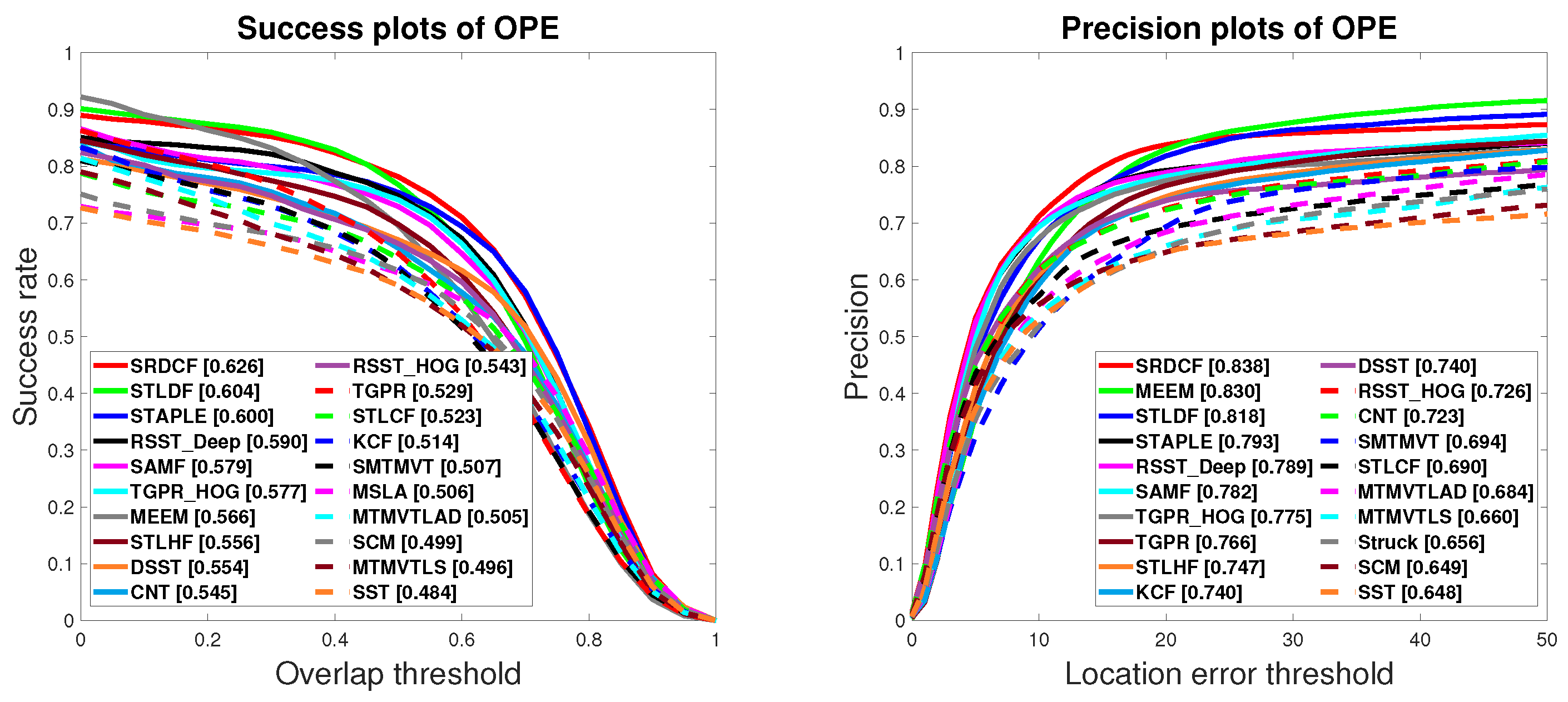
4.2. Experimental Results on OTB50

This benchmark consists of 50 annotated sequences, where 49 sequences have one annotated target and one sequence (jogging) has two annotated targets [39]. We evaluate the overall performance of the proposed STLDF and its two variants (i.e., STLCF and STLHF) against 29 baseline trackers in Reference [39] and 17 recent trackers including MTMVTLS [43], MTMVTLAD [13], MSLA [14] (the recent version of ASLA [34]), SST [5], SMTMVT [44], CNT [21], two variants of TGPR (i.e., TGPR_Color and TGPR_HOG) [45], DSST [46], PCOM [47], KCF [19], MEEM [48], SAMF [49], SRDCF [50], STAPLE [51], and two variants of RSST (i.e., RSST_HOG and RSST_Deep) [23]. We present the overall OPE success and precision plots in Figure 2. We only include top 20 of the 49 compared trackers in each plot to avoid clutter and increase the readability. The value within the parenthesis alongside each legend of the success plots is the AUC score for the corresponding tracker. Similarly, the value within the parenthesis alongside each legend of the precision plots is the precision score for the corresponding tracker.

It is clear from Figure 2 that incorporating deep features improves the tracking performance as the proposed STLDF achieves better AUC and precision scores than its two variants, that is, STLHF and STLCF. The similar improvement trends are also observed in Reference [23], where RSST_Deep achieves better performance than RSST_HOG. Among the 29 baseline trackers employed in Reference [39], SCM [52] and Struck [53] achieve the most favorable performance. STLDF significantly improves both baseline trackers. Specifically, it outperforms SCM and Struck by 21.04% and 24.73% in terms of the AUC scores, respectively. It outperforms SCM and Struck by 26.04% and 24.70% in terms of the precision scores, respectively. When comparing with the 17 additional recent trackers, STLDF achieves higher AUC scores than 16 of these trackers and a comparable score as SRDCF (the best tracker in comparison). Specifically, it improves the AUC scores of MTMVTLAD, MSLA, KCF, CNT, DSST, MEEM, TGPR_HOG, SAMF, RSST_Deep, and STAPLE by 19.60%, 19.37%, 17.51%, 10.83%, 9.03%, 6.71%, 4.68%, 4.32%, 2.37%, and 0.67%, respectively. SRDCF shows slightly better performance than STLDF (0.626 AUC score for SRDCF vs. 0.604 AUC score for STLDF). STLDF also achieves higher precision scores than 15 out of 17 additional recent trackers. Specifically, it outperforms MTMVTLAD, SMTMVT, CNT, DSST, KCF, TGPR_HOG, SAMF, RSST_Deep, and STAPLE by 19.59%, 17.87%, 13.14%, 10.54%, 10.54%, 5.55%, 4.60%, 3.68%, and 3.15%, respectively. It attains a comparable precision score as MEEM and SRDCF. All three trackers yields the precision scores above 0.81.

To demonstrate the effectiveness of the proposed optimization model, we compare the proposed tracker and its two variants (i.e., STLDF, STLHF, and STLCF) with representative traditional and recent sparse trackers in terms of the two evaluation metrics in

Table 1. Summary of the tracking performance of the proposed tracker, its two variants, and nine representative sparse trackers on OTB50. Bold numbers indicate the highest area under curve (AUC) and precision scores (i.e., the best tracking performance).

Score	L1APG	ASLA	MTT	MTMVTLAD	MSLA	SST	RSST			Proposed Method
							Color	HOG	Deep	STLCF	STLHF	STLDF
AUC	0.380	0.434	0.376	0.505	0.506	0.484	0.520	0.543	0.590	0.523	0.556	0.604
Precision	0.485	0.532	0.479	0.684	0.631	0.648	0.691	0.726	0.789	0.690	0.747	0.818

. It is clear that STLDF achieves the highest overall AUC and precision scores among all the compared sparse trackers. It improves RSST_Deep, one of the most recent sparse trackers that incorporates the deep features, by 2.37% in the AUC score and 3.68% in the precision score. Its two variants (STLHF, and STLCF) also outperforms RSST’s counterparts (RSST_HOG, and RSST_ Color) in terms of two evaluation metrics except that STLCF achieves the similar precision score as RSST_Color (0.690 vs. 0.691). In addition, STLCF achieves higher AUC and precision scores than other sparse trackers that utilize intensity features such as L1APG [54], ASLA [34], MTT [55], MSLA [14], and SST [5]. STLHF also achieves higher AUC and precision scores than the sparse trackers that utilize HOG features such as MTMVTLAD [13] and RSST_HOG [23]. It is worthy of mentioning that the proposed method attains significant improvements over conventional local sparse trackers (ASLA and MSLA) by preserving the spatial layout structures among different local patch features inside a target candidate. The robust tracking performance of the proposed method demonstrate the effectiveness of the proposed optimization model that employs a group-sparsity regularization term to adopt local and spatial information of the target candidates and attain the spatial layout structure among them.

In addition to sparse trackers, the proposed STLDF achieves a better or comparable AUC score (0.604) than some correlation filter (CF) based trackers including KCF (0.514) [19], DSST (0.556) [46], LCT (0.612) [56], HDT (0.603) [20], CF2 (0.605) [37], and ACFN (0.607) [57]. It also achieves a better or comparable precision score (0.818) than the following CF-based trackers: KCF (0.740), DSST (0.740), LCT (0.848), HDT (0.889), CF2 (0.891), and ACFN (0.860).

Comparing with deep learning-based trackers, the proposed STLDF outperforms or achieves a comparable AUC score than CNT (0.545) [21], GOTURN (0.444) [58], CNN-SVM (0.597) [25], FCNT (0.599) [18], DLSSVM (0.589) [22], and SiamFC (0.608) [59]. Moreover, it outperforms or achieves comparable precision score than CNT (0.723), GOTURN (0.620), CNN-SVM (0.852), FCNT (0.856), DLSSVM (0.829), and SiamFC (0.815).

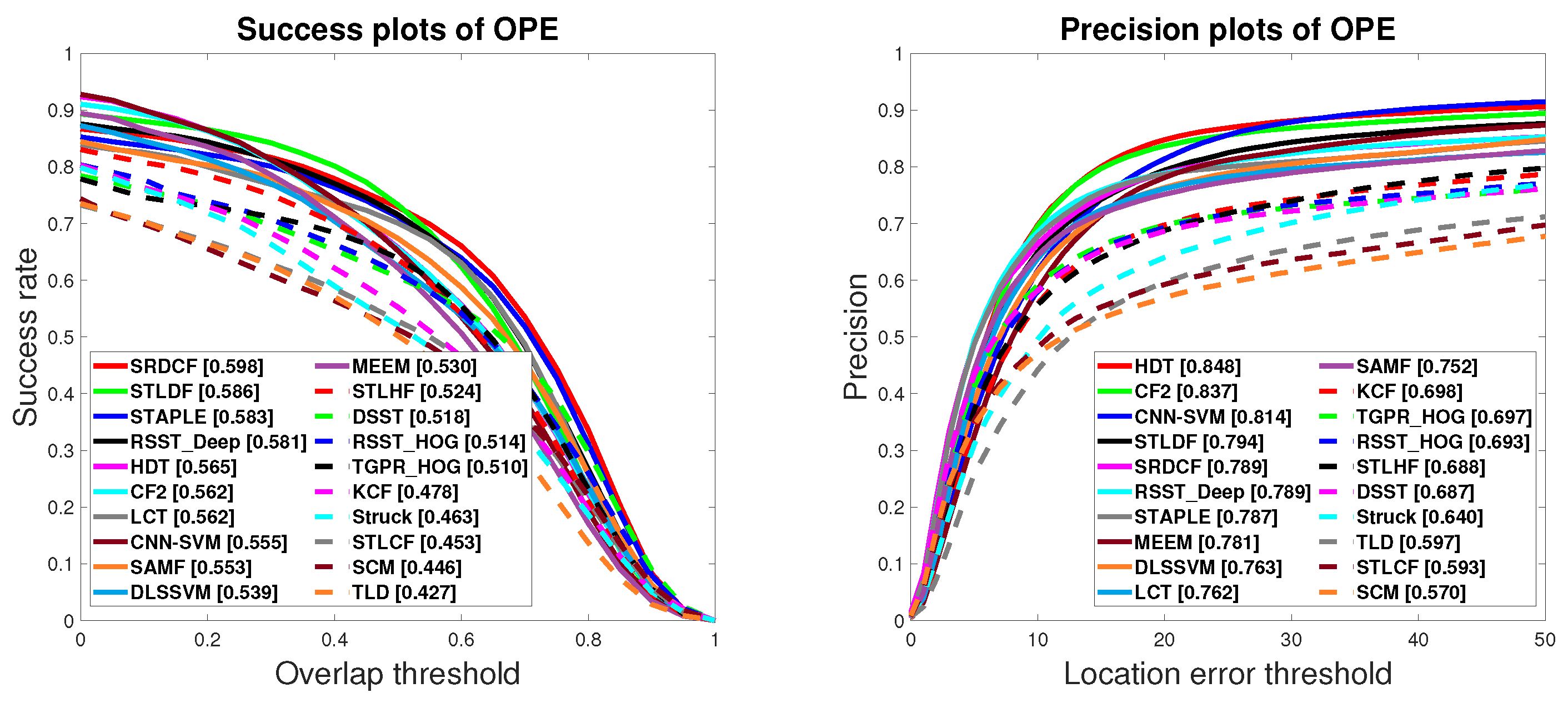
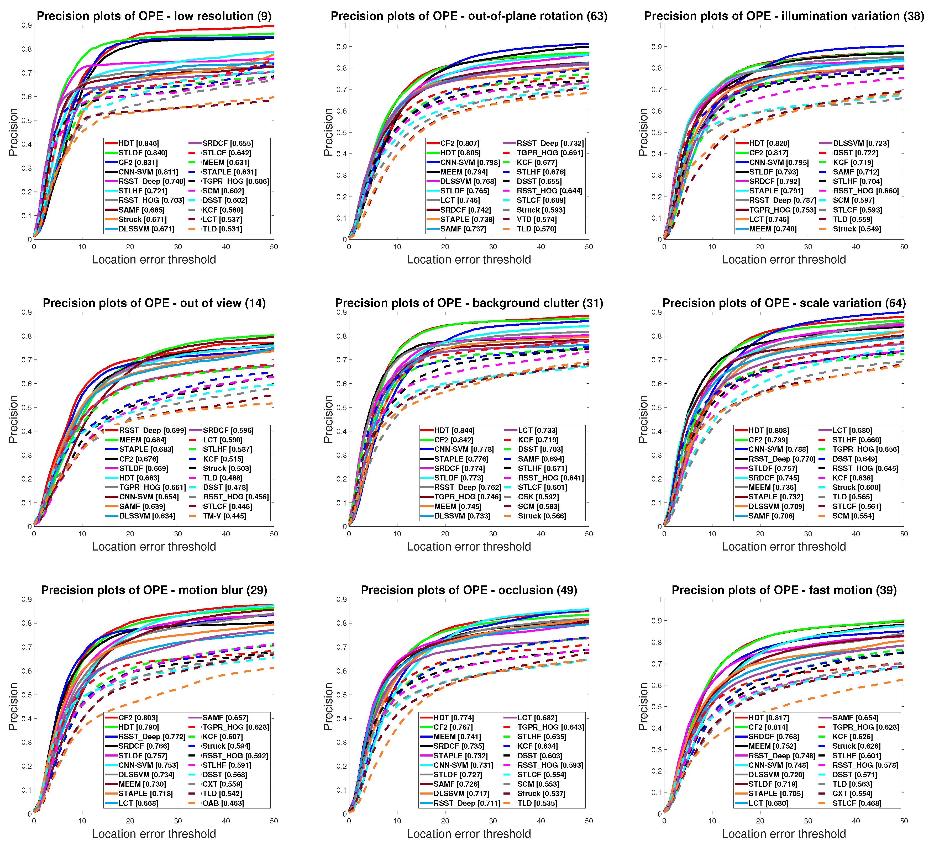
4.3. Experimental Results on OTB100

OTB100 [40] is an extension of OTB50 [39] by adding 50 additional annotated sequences. Two sequences, jogging and Skating, have two annotated targets. The rest of the sequences have one annotated target. Each sequence is also labeled with challenge attributes such as illumination variation (IV), scale variation (SV), occlusion (OCC), deformation (DEF), motion blur (MB), fast motion (FM), in-plane rotation (IPR), out-of-plane rotation (OPR), out-of-view (OV), background clutter (BC), and low resolution (LR). The sequences are categorized based on the attributes and 11 challenge subsets are generated. These subsets are utilized to evaluate the performance of trackers in different challenge categories.

We evaluate the proposed STLDF and its two variants (STLHF and STLCF) against 29 baseline trackers in Reference [40], and 15 recent trackers including DSST, PCOM, KCF, TGPR_HOG, MEEM, SAMF, SRDCF, LCT, STAPLE, CF2, CNN-SVM, DLSSVM, HDT, and two variants of RSST (i.e., RSST_HOG and RSST_Deep). Some trackers used in the experiments of OTB50 are excluded from this experiment since they do not publish their results on OTB100. Similar to the experiments on OTB50, we follow standard protocols proposed in References [39,40] and use the same parameters on all sequences to obtain the OPE results. We present the overall OPE success and precision plots of the top 20 trackers out of 47 compared trackers in Figure 3.

It is clear from Figure 3 that the proposed STLDF achieves higher AUC and precision scores than its two variants for 100 sequences in OTB100 due to its utility of local deep features. It also achieves higher AUC and precision scores than RSST_Deep due to its novel optimization model. Similar to the tracking results obtained on OTB50, SCM and Struck are the top two trackers among the 29 baseline trackers on OTB100. STLDF improves the AUC scores of SCM and Struck by 31.39% and 26.57% and the precision scores of SCM and Struck by 39.30% and 24.06%, respectively. Compared to the 15 recent trackers, STLDF achieves comparable AUC scores as SRDCF (0.586 vs. 0.598) and improves the AUC scores of the remaining 14 trackers. Specifically, it improves the AUC scores of the top 13 trackers, namely, KCF, TGPR_HOG, RSST_HOG, DSST, MEEM, DLSSVM, SAMF, CNN-SVM, LCT, CF2, HDT, RSST_Deep, and STAPLE by 22.59%, 14.90%, 14.01%, 13.13%, 10.57%, 8.72%, 5.97%, 5.59%, 4.27%, 4.27%, 3.72%, ,0.87%, and 0.52%, respectively. It also significantly improves the precision scores of six of these 15 trackers including SST, TGPR_HOG, KCF, SAMF, LCT, and DLSSVM by 15.57%, 13.92%, 13.75%, 5.59%, 4.20%, and 4.06%, respectively. In addition, it achieves a little bit improvement over four trackers including MEEM, STAPLE, RSST_Deep, and SRDCF. It is inferior to three trackers such as HDT, CF2, and CNN-SVM by a small margin.

The proposed STLDF significantly outperforms conventional sparse trackers such as L1APG [54], LRST [60], ASLA [34], and MTT [55] and improves both AUC and precision scores of RSST_Deep [23], one of the most recent sparse trackers, by 0.87% and 0.64%, respectively. STLDF with the achieved AUC score of 0.586 outperforms some CF-based trackers such as KCF (0.478), DSST (0.518), LCT (0.562), CF2 (0.562), and HDT (0.565) and some deep learning-based trackers such as GOTURN (0.427), CNN-SVM (0.555), and DLSSVM (0.539). These OTB100 tracking results follow the similar trends in OTB50 tracking results and demonstrate the effectiveness of the proposed optimization model and the integration of local deep features.

We further evaluate the performance of STLDF in terms of AUC and precision scores on nine challenge subsets including LR, OPR, IV, OV, BC, SV, MB, OCC, and FM. Figure 4 and Figure 5 show the success and precision plots of top 20 trackers for these 9 challenge subsets, respectively. The value within the parenthesis on the title line of each plot is the number of video sequences in the specific subset. The value within the parenthesis alongside each legend of the success plot is the AUC score for the corresponding tracker and the value within the parenthesis alongside each legend of the precision plots is the precision score for the corresponding tracker. It is clear that STLDF achieves significantly better performance than its two variants (STLHF and STLCF) due to its integration of local deep features. As it is shown in Figure 4, STLDF ranks the best for two subsets with LR and OPR challenges, the second for two subsets with IV and OV challenges, the third for three subsets with BC, SV, and MB challenges, the fourth for the OCC subset, and the top sixth tracker for FM challenge in terms of ACU score. As it is demonstrated in Figure 5, STLDF ranks as one of the top five trackers for five subsets with LR, IV, OV, SV, and MB, the sixth best trackers in OPR and BC, and the top eight trackers for two subsets with OCC and FM challenges in terms of the precision scores. The DEF and IPR challenge subsets are not included in Figure 4 and Figure 5 due to lack of space. STLDF obtains the AUC and precision scores of 0.529 (6th rank) and 0.727 (7th rank) for the DEF subset, respectively. STLDF yields the AUC and precision scores of 0.543 (8th rank) and 0.742 (10th rank) for the IPR challenge subset, respectively.

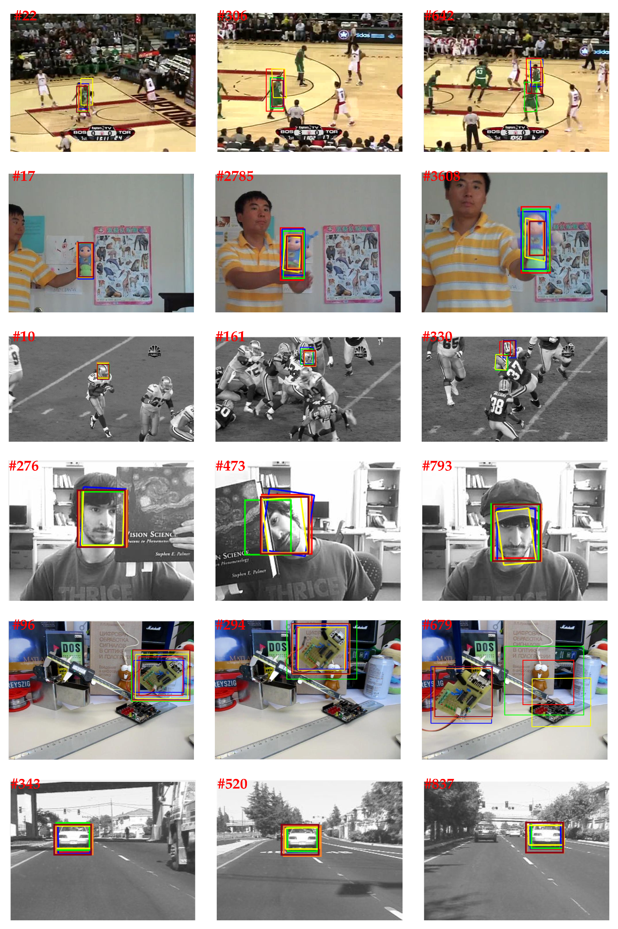
4.4. Qualitative Results

In this section, we provide the qualitative results of the proposed STLDF tracker on several representative frame sequences in the OTB100 dataset. We compare the performance of STLDF with the top five trackers, namely, SRDCF, Staple, RSST_Deep, HDT, and CF2, on the OTB100 benchmark. Figure 6 presents the tracking results of the compared methods on six OTB100 frame sequences including basketball, doll, football, faceOcc2, board, and car2. Each of these six frame sequences has its challenges as summarized below:

• basketball: IV, OCC, DEF, OPR, BC;
• doll: IV, SV, OCC, IPR, OPR;
• football: OCC, IPR, OPR, BC;
• faceOcc2: IV, OCC, IPR, OPR;
• board: SV, MB, FM, OPR, OV, BC;
• car2: IV, SV, MB, FM, BC.

Here, we briefly analyze the tracking performance of each compared tracker under different challenging scenarios. For the basketball sequence, all six trackers except Staple are able to track the basketball player till the end. However, SRDCF drifts from the player in some frames and RSST_Deep under-estimates the scale of the player. For the doll sequence, all six trackers are able to track the doll over time. However, CF2, HDT and RSST_Deep fail to estimate the scales of the doll throughout the sequence. For the football sequence, RSST_Deep and Staple track the wrong face towards the end. For the faceOcc2 sequence, all six trackers successfully handle the face occlusions. RSST_Deep handles the rotation of the face more robustly compared to other trackers. For the board sequence, Staple, RSST_Deep, and SRDCF lose the board when it undergoes various rotations and scale variations in a cluttered background. For the car2 sequence, SRDCF and STLDF are able to handle the illumination variation and scale variation more robustly than the other trackers as the car reaches to the end of frame sequence.

4.5. Discussions

The proposed STLDF has demonstrated superior tracking performance in terms of overall success and precision plots in comparison to representative conventional and recent sparse trackers [5,13,14,23,54]. It outperforms one of the most recent and powerful sparse trackers, RSST_Deep [23], in both OTB50 and OTB100. Specifically, it attains better performance than RSST_Deep when the target undergoes various challenges such as deformation, illumination variation, low resolution, occlusion, and out of plane rotations. However, similar to the other sparse trackers, STLDF is less effective in handling targets with fast motion and motion blur, mainly due to the inefficiency of its particle filter resampling process to handle the fast motions of targets between consecutive frames.

The proposed STLDF has also demonstrated superior tracking performance in comparison to some state-of-the-art CF trackers [20,37,46]. However, sparse trackers are more computational expensive than CF trackers since they have to solve an optimization model in each frame to find the target among a number of candidates. On the contrary, CF trackers use the fast Fourier transform to efficiently distinguish the target from backgrounds. Furthermore, sparse trackers can barely recover successfully when drifts occur mainly due to the following two reasons: (1) The particle filter resampling is limited around the location of tracked target in the previous frame. (2) The templates are updated with a wrong tracking result. Both lead to the error propagates throughout the sequence. In future, we will investigate an adaptive template update and particle filter resampling process to address this shortcoming and improve the performance of STLDF.

5. Conclusions and Future Work

We propose a structured tracker using local deep features (STLDF), which exploits CNN deep features of local patches within target candidates and represents them in a novel optimization problem. The proposed optimization model combines the CNN deep features of local patches of each target candidate with a group-sparsity regularization term to encourage the tracker to sparsely select appropriate local patches of the same subset of templates. We design a fast and parallel numerical algorithm by deriving the augmented Lagrangian of the optimization model into two close-form problems: the quadratic problem and the Euclidean norm projection onto probability simplex constraints problem. STLDF outperforms existing sparse trackers by incorporating local deep features of target candidates and maintaining the spatial relation between them. The extensive experimental results on OTB50 and OTB100 demonstrate that STLDF outperforms various state-of-the-art methods including its two variant trackers, representative conventional and recent sparse trackers, correlation filter-based trackers, and convolutional neural network based trackers in terms of AUC and precision scores.

In the future, we will investigate the effect of different interpolation techniques on the tracking results. We will also employ different norms in the objective function and develop their corresponding numerical methods to solve the tracking problem.

References

1. Yilmaz, A.; Javed, O.; Shah, M. Object tracking: A survey. Acm Comput. Surv. (CSUR) 2006, 38, 13. [Google Scholar] [CrossRef]
2. Salti, S.; Cavallaro, A.; Di Stefano, L. Adaptive appearance modeling for video tracking: Survey and evaluation. IEEE Trans. Image Process. 2012, 21, 4334–4348. [Google Scholar] [CrossRef] [PubMed]
3. Pang, Y.; Ling, H. Finding the best from the second bests-inhibiting subjective bias in evaluation of visual tracking algorithms. In Proceedings of the IEEE International Conference on Computer Vision, Portland, OR, USA, 23–28 June 2013; pp. 2784–2791. [Google Scholar]
4. Kristan, M.; Matas, J.; Leonardis, A.; Felsberg, M.; Cehovin, L.; Fernandez, G.; Vojir, T.; Hager, G.; Nebehay, G.; Pflugfelder, R. The visual object tracking vot2015 challenge results. In Proceedings of the 2015 IEEE International Conference on Computer Vision workshops (ICCV), Araucano, Park Las Condes, Chile, 11–18 December 2015; pp. 1–23. [Google Scholar]
5. Zhang, T.; Liu, S.; Xu, C.; Yan, S.; Ghanem, B.; Ahuja, N.; Yang, M.H. Structural sparse tracking. In Proceedings of the 2015 IEEE Conference on Computer Vision and Pattern Recognition (CVPR), Boston, MA, USA, 7–12 June 2015; pp. 150–158. [Google Scholar]
6. Zhang, T.; Bibi, A.; Ghanem, B. In defense of sparse tracking: Circulant sparse tracker. In Proceedings of the 2016 IEEE Conference on Computer Vision and Pattern Recognition (CVPR), Las Vegas, NV, USA, 27–30 June 2016; pp. 3880–3888. [Google Scholar]
7. Avidan, S. Ensemble tracking. IEEE Trans. Pattern Anal. Mach. Intell. 2007, 29, 261–271. [Google Scholar] [CrossRef] [PubMed]
8. Grabner, H.; Leistner, C.; Bischof, H. Semi-supervised on-line boosting for robust tracking. In European Conference on Computer Vision (ECCV); Springer: Berlin/Heidelberg, Germany, 2008; pp. 234–247. [Google Scholar]
9. Babenko, B.; Yang, M.H.; Belongie, S. Visual tracking with online multiple instance learning. In Proceedings of the 2009 IEEE Conference on Computer Vision and Pattern Recognition (CVPR), Miami, FL, USA, 20–25 June 2009; pp. 983–990. [Google Scholar]
10. Black, M.J.; Jepson, A.D. Eigentracking: Robust matching and tracking of articulated objects using a view-based representation. Int. J. Comput. Vis. 1998, 26, 63–84. [Google Scholar] [CrossRef]
11. Ross, D.A.; Lim, J.; Lin, R.S.; Yang, M.H. Incremental learning for robust visual tracking. Int. J. Comput. Vis. 2008, 77, 125–141. [Google Scholar] [CrossRef]
12. Mei, X.; Ling, H. Robust visual tracking and vehicle classification via sparse representation. IEEE Trans. Pattern Anal. Mach. Intell. 2011, 33, 2259–2272. [Google Scholar] [PubMed] [Green Version]
13. Mei, X.; Hong, Z.; Prokhorov, D.; Tao, D. Robust multitask multiview tracking in videos. IEEE Trans. Neural Netw. Learn. Syst. 2015, 26, 2874–2890. [Google Scholar] [CrossRef] [PubMed]
14. Jia, X.; Lu, H.; Yang, M.H. Visual tracking via coarse and fine structural local sparse appearance models. IEEE Trans. Image Process. 2016, 25, 4555–4564. [Google Scholar] [CrossRef] [PubMed]
15. Ojala, T.; Pietikäinen, M.; Mäenpää, T. Multiresolution gray-scale and rotation invariant texture classification with local binary patterns. IEEE Trans. Pattern Anal. Mach. Intell. 2002, 971–987. [Google Scholar]
16. Dalal, N.; Triggs, B. Histograms of oriented gradients for human detection. In Proceedings of the 2005 IEEE Computer Society Conference on Computer Vision and Pattern Recognition (CVPR), San Diego, CA, USA, 20–25 June 2005; Volume 1, pp. 886–893. [Google Scholar]
17. Wang, N.; Yeung, D.Y. Learning a deep compact image representation for visual tracking. In Advances in Neural Information Processing Systems, Proceedings of the 27th Annual Conference on Neural Information Processing Systems (NIPS), Lake Tahoe, NV, USA, 5–8 December 2013; Neural Information Processing Systems Foundation, Inc.: San Diego, CA, USA, 2013; pp. 809–817. [Google Scholar]
18. Wang, L.; Ouyang, W.; Wang, X.; Lu, H. Visual tracking with fully convolutional networks. In Proceedings of the 2012 IEEE Conference on Computer Vision and Pattern Recognition (CVPR), Boston, MA, USA, 7–12 June 2015; pp. 3119–3127. [Google Scholar]
19. Henriques, J.F.; Caseiro, R.; Martins, P.; Batista, J. High-speed tracking with kernelized correlation filters. IEEE Trans. Pattern Anal. Mach. Intell. 2015, 37, 583–596. [Google Scholar] [CrossRef] [PubMed] [Green Version]
20. Qi, Y.; Zhang, S.; Qin, L.; Yao, H.; Huang, Q.; Lim, J.; Yang, M.H. Hedged deep tracking. In Proceedings of the 2012 IEEE Conference on Computer Vision and Pattern Recognition (CVPR), Las Vegas, NV, USA, 27–30 June 2016; pp. 4303–4311. [Google Scholar]
21. Zhang, K.; Liu, Q.; Wu, Y.; Yang, M.H. Robust visual tracking via convolutional networks without training. IEEE Trans. Image Process. 2016, 25, 1779–1792. [Google Scholar] [CrossRef] [PubMed]
22. Ning, J.; Yang, J.; Jiang, S.; Zhang, L.; Yang, M.H. Object tracking via dual linear structured SVM and explicit feature map. In Proceedings of the 2012 IEEE Conference on Computer Vision and Pattern Recognition (CVPR), Las Vegas, NV, USA, 27–30 June 2016; pp. 4266–4274. [Google Scholar]
23. Zhang, T.; Xu, C.; Yang, M.H. Robust structural sparse tracking. IEEE Trans. Pattern Anal. Mach. Intell. 2018, 41, 473–486. [Google Scholar] [CrossRef] [PubMed]
24. Wang, L.; Liu, T.; Wang, G.; Chan, K.L.; Yang, Q. Video tracking using learned hierarchical features. IEEE Trans. Image Process. 2015, 24, 1424–1435. [Google Scholar] [CrossRef] [PubMed]
25. Hong, S.; You, T.; Kwak, S.; Han, B. Online tracking by learning discriminative saliency map with convolutional neural network. In Proceedings of the International Conference on Machine Learning, Lille, France, 6–11 July 2015; pp. 597–606. [Google Scholar]
26. Wang, N.; Li, S.; Gupta, A.; Yeung, D.Y. Transferring rich feature hierarchies for robust visual tracking. arXiv 2015, arXiv:1501.04587. [Google Scholar]
27. Simonyan, K.; Zisserman, A. Very deep convolutional networks for large-scale image recognition. arXiv 2014, arXiv:1409.1556. [Google Scholar]
28. Nam, H.; Han, B. Learning multi-domain convolutional neural networks for visual tracking. In Proceedings of the 2012 IEEE Conference on Computer Vision and Pattern Recognition (CVPR), Las Vegas, NV, USA, 27–30 June 2016; pp. 4293–4302. [Google Scholar]
29. Jung, I.; Son, J.; Baek, M.; Han, B. Real-Time MDNet. arXiv 2018, arXiv:1808.08834. [Google Scholar]
30. Nam, H.; Baek, M.; Han, B. Modeling and propagating cnns in a tree structure for visual tracking. arXiv 2016, arXiv:1608.07242. [Google Scholar]
31. Song, Y.; Ma, C.; Wu, X.; Gong, L.; Bao, L.; Zuo, W.; Shen, C.; Lau, R.W.; Yang, M.H. Vital: Visual tracking via adversarial learning. In Proceedings of the IEEE Conference on Computer Vision and Pattern Recognition, Salt Lake City, UT, USA, 18–21 June 2018; pp. 8990–8999. [Google Scholar]
32. Pu, S.; Song, Y.; Ma, C.; Zhang, H.; Yang, M.H. Deep attentive tracking via reciprocative learning. In Advances in Neural Information Processing Systems, Proceedings of the Annual Conference on Neural Information Processing Systems, Montreal, QC, Canada, 3–8 December 2018; MIT Press: Cambridge, MA, USA, 2018; pp. 1931–1941. [Google Scholar]
33. Javanmardi, M.; Qi, X. Structured group local sparse tracker. IET Image Process. 2019, 13, 1391–1399. [Google Scholar] [CrossRef] [Green Version]
34. Jia, X.; Lu, H.; Yang, M.H. Visual tracking via adaptive structural local sparse appearance model. In Proceedings of the 2012 IEEE Conference on Computer Vision and Pattern Recognition (CVPR), Providence, RI, USA, 16–21 June 2012; pp. 1822–1829. [Google Scholar]
35. Boyd, S.; Parikh, N.; Chu, E.; Peleato, B.; Eckstein, J. Distributed optimization and statistical learning via the alternating direction method of multipliers. Found. Trends® Mach. Learn. 2011, 3, 1–122. [Google Scholar]
36. Deng, J.; Dong, W.; Socher, R.; Li, L.J.; Li, K.; Li, F.-F. Imagenet: A large-scale hierarchical image database. In Proceedings of the 2009 IEEE Conference on Computer Vision and Pattern Recognition, Miami, FL, USA, 20–25 June 2009; pp. 248–255. [Google Scholar]
37. Ma, C.; Huang, J.B.; Yang, X.; Yang, M.H. Hierarchical convolutional features for visual tracking. In Proceedings of the 2012 IEEE Conference on Computer Vision and Pattern Recognition (CVPR), Boston, MA, USA, 7–12 June 2015; pp. 3074–3082. [Google Scholar]
38. Redmon, J.; Divvala, S.; Girshick, R.; Farhadi, A. You only look once: Unified, real-time object detection. In Proceedings of the 2012 IEEE Conference on Computer Vision and Pattern Recognition (CVPR), Las Vegas, NV, USA, 27–30 June 2016; pp. 779–788. [Google Scholar]
39. Wu, Y.; Lim, J.; Yang, M.H. Online object tracking: A benchmark. In Proceedings of the 2013 IEEE Conference on Computer Vision and Pattern Recognition, Portland, OR, USA, 23–28 June 2013; pp. 2411–2418. [Google Scholar]
40. Wu, Y.; Lim, J.; Yang, M.H. Object tracking benchmark. IEEE Trans. Pattern Anal. Mach. Intell. 2015, 37, 1834–1848. [Google Scholar] [CrossRef] [PubMed] [Green Version]
41. Henriques, J.F.; Caseiro, R.; Martins, P.; Batista, J. Exploiting the circulant structure of tracking-by-detection with kernels. In European Conference on Computer Vision; Springer: Berlin/Heidelberg, Germany, 2012; pp. 702–715. [Google Scholar]
42. Vedaldi, A.; Lenc, K. Matconvnet: Convolutional neural networks for matlab. In Proceedings of the 23rd ACM International Conference on Multimedia, Brisbane, Australia, 26–30 October 2015; ACM: New York, NY, USA, 2015; pp. 689–692. [Google Scholar]
43. Hong, Z.; Mei, X.; Prokhorov, D.; Tao, D. Tracking via robust multi-task multi-view joint sparse representation. In Proceedings of the 2013 IEEE Conference on Computer Vision and Pattern Recognition, Portland, OR, USA, 23–28 June 2013; pp. 649–656. [Google Scholar]
44. Javanmardi, M.; Qi, X. Robust Structured Multi-Task Multi-View Sparse Tracking. In Proceedings of the 2018 IEEE International Conference on Multimedia and Expo (ICME), San Diego, CA, USA, 23–27 July 2018; pp. 1–6. [Google Scholar] [CrossRef] [Green Version]
45. Gao, J.; Ling, H.; Hu, W.; Xing, J. Transfer learning based visual tracking with gaussian processes regression. In European Conference on Computer Vision; Springer: Zurich, Switzerland, 2014; pp. 188–203. [Google Scholar]
46. Danelljan, M.; Häger, G.; Khan, F.; Felsberg, M. Accurate scale estimation for robust visual tracking. In Proceedings of the British Machine Vision Conference, Nottingham, UK, 1–5 September 2014; BMVA Press: Durham, UK, 2014. [Google Scholar]
47. Wang, D.; Lu, H. Visual tracking via probability continuous outlier model. In Proceedings of the 27th IEEE Conference on Computer Vision and Pattern Recognition (CVPR), Columbus, OH, USA, 24–27 June 2014; pp. 3478–3485. [Google Scholar]
48. Zhang, J.; Ma, S.; Sclaroff, S. MEEM: robust tracking via multiple experts using entropy minimization. In Proceedings of the 13th European Conference, Zurich, Switzerland, 6–12 September 2014. [Google Scholar]
49. Li, Y.; Zhu, J. A scale adaptive kernel correlation filter tracker with feature integration. In European Conference on Computer Vision; Springer: Zuric, Switzerland, 2014; pp. 254–265. [Google Scholar]
50. Danelljan, M.; Hager, G.; Shahbaz Khan, F.; Felsberg, M. Learning spatially regularized correlation filters for visual tracking. In Proceedings of the 2012 IEEE Conference on Computer Vision and Pattern Recognition (CVPR), Boston, MA, USA, 7–12 June 2015; pp. 4310–4318. [Google Scholar]
51. Bertinetto, L.; Valmadre, J.; Golodetz, S.; Miksik, O.; Torr, P.H. Staple: Complementary learners for real-time tracking. In Proceedings of the 2012 IEEE Conference on Computer Vision and Pattern Recognition (CVPR), Las Vegas, NV, USA, 27–30 June 2016; pp. 1401–1409. [Google Scholar]
52. Zhong, W.; Lu, H.; Yang, M.H. Robust object tracking via sparsity-based collaborative model. In Proceedings of the 2012 IEEE Conference on Computer Vision and Pattern Recognition (CVPR), Providence, RI, USA, 16–21 June 2012; pp. 1838–1845. [Google Scholar]
53. Hare, S.; Golodetz, S.; Saffari, A.; Vineet, V.; Cheng, M.M.; Hicks, S.L.; Torr, P.H. Struck: Structured output tracking with kernels. IEEE Trans. Pattern Anal. Mach. Intell. 2016, 38, 2096–2109. [Google Scholar] [CrossRef] [PubMed] [Green Version]
54. Bao, C.; Wu, Y.; Ling, H.; Ji, H. Real time robust l1 tracker using accelerated proximal gradient approach. In Proceedings of the 2012 IEEE Conference on Computer Vision and Pattern Recognition (CVPR), Providence, RI, USA, 16–21 June 2012; pp. 1830–1837. [Google Scholar]
55. Zhang, T.; Ghanem, B.; Liu, S.; Ahuja, N. Robust visual tracking via multi-task sparse learning. In Proceedings of the 2012 IEEE Conference on Computer Vision and Pattern Recognition (CVPR), Providence, RI, USA, 16–21 June 2012; pp. 2042–2049. [Google Scholar]
56. Ma, C.; Yang, X.; Zhang, C.; Yang, M.H. Long-term correlation tracking. In Proceedings of the 2015 IEEE Conference on Computer Vision and Pattern Recognition (CVPR), Boston, MA, USA, 7–12 June 2015; pp. 5388–5396. [Google Scholar]
57. Choi, J.; Chang, H.J.; Yun, S.; Fischer, T.; Demiris, Y.; Choi, J.Y. Attentional Correlation Filter Network for Adaptive Visual Tracking. In Proceedings of the Conference on Computer Vision and Pattern Recognition (CVPR), Honolulu, HI, USA, 21–26 July 2017; Volume 2, p. 7. [Google Scholar]
58. Held, D.; Thrun, S.; Savarese, S. Learning to track at 100 fps with deep regression networks. In European Conference on Computer Vision; Springer: Amsterdam, The Netherlands, 2016; pp. 749–765. [Google Scholar]
59. Bertinetto, L.; Valmadre, J.; Henriques, J.F.; Vedaldi, A.; Torr, P.H. Fully-convolutional siamese networks for object tracking. In European Conference on Computer Vision; Springer: Amsterdam, The Netherlands, 2016; pp. 850–865. [Google Scholar]
60. Zhang, T.; Ghanem, B.; Liu, S.; Ahuja, N. Low-rank sparse learning for robust visual tracking. In European Conference on Computer Vision; Springer: Berlin/Heidelberg, Germany, 2012; pp. 470–484. [Google Scholar]
Figure 1. The overview of the proposed STLDF method.
Electronics 09 00846 g001
Figure 2. The overall one pass evaluation (OPE) plots for 50 frame sequences in OTB50.
Electronics 09 00846 g002
Figure 3. The overall OPE plots for 100 frame sequences in OTB100.
Electronics 09 00846 g003
Figure 4. The OPE success plots for LR, OPR, IV, OV, BC, SV, MB, OCC, and FM subsets in OTB100.
Electronics 09 00846 g004
Figure 5. The OPE precision plots for LR, OPR, IV, OV, BC, SV, MB, OCC, and FM subsets in OTB100.
Electronics 09 00846 g005
Figure 6. Comparison of the tracking results of the proposed STLDF and top five state-of-the-art trackers on basketball, doll, football, faceOcc2, board, and car2 image sequences. Frame indices are shown at the top left corner of each representative frame. Results are best viewed on high-resolution displays. (CF2, HDT, RSST_Deep, Staple, SRDCF, STLDF).
Electronics 09 00846 g006