Detecting Predictable Segments of Chaotic Financial Time Series via Neural Network

Abstract

In this study, a new idea is proposed to analyze the financial market and detect price fluctuations, by integrating the technology of PSR (phase space reconstruction) and SOM (self organizing maps) neural network algorithms. The prediction of price and index in the financial market has always been a challenging and significant subject in time-series studies, and the prediction accuracy or the sensitivity of timely warning price fluctuations plays an important role in improving returns and avoiding risks for investors. However, it is the high volatility and chaotic dynamics of financial time series that constitute the most significantly influential factors affecting the prediction effect. As a solution, the time series is first projected into a phase space by PSR, and the phase tracks are then sliced into several parts. SOM neural network is used to cluster the phase track parts and extract the linear components in each embedded dimension. After that, LSTM (long short-term memory) is used to test the results of clustering. When there are multiple linear components in the m-dimension phase point, the superposition of these linear components still remains the linear property, and they exhibit order and periodicity in phase space, thereby providing a possibility for time series prediction. In this study, the Dow Jones index, Nikkei index, China growth enterprise market index and Chinese gold price are tested to determine the validity of the model. To summarize, the model has proven itself able to mark the unpredictable time series area and evaluate the unpredictable risk by using 1-dimension time series data.

1. Introduction

Recently, nonlinear models, such as LSTM and deep learning algorithms, have been widely used and proven effective to train and predict time series [1,2,3]. However, it is the outstanding prediction results which are contrary to the initial sensitivity law of chaotic system and the principle of long-term immeasurability [4]. The fact is, the dynamic properties of a chaotic financial time series should be restored first before it is analyzed. For example, by calculating the Hurst index with MF-DFA [5], or using PSR technology to restore the dynamic system of time series, and calculate the Lyapunov index and K entropy, the complexity of time series and the size of predictable range of time series needs to be acquired [6]. The chaos degree of a time series system can be described with Lyapunov index, which means that the more chaotic the system is, the more difficult it is to predict the time series. Besides, the predictable range of a time series is reflected by the reciprocal of the Lyapunov index. If the Lyapunov index is greater than 1, the prediction ability of the time series is less than one step, which means that the data in the past is not highly correlated with the data to be generated in the future [7]. It is meaningful to predict the time series only when the Lyapunov index is $0<L<1$. When the Hurst index is in the range of $0<h<0.5$, it indicates that the time series has a long-term correlation, although the future trend is opposite to the past trend [6]. The closer h is to 0, the stronger the negative correlation of price is. When h is close to $0.5$, the time series is random or uncorrelated, which means the past data will not affect the future data. Instead of directly fitting and predicting time series with nonlinear models, the methods above should be considered as preconditions for predicting time series, as they are the solutions to over-fitting.

In our past study, real financial data DJI, SSE, Nikkei and DAX were reconstructed and by PSR to restore the dynamic properties of the time series [4]. The study concluded that a time series is a chaotic system, and it cannot be predicted for a long time. Here are the two main points of our past study: 1. A time series can be predicted in the short term, and the prediction range is limited by the degree of chaos. 2. Although time series show disorder and randomness in the time domain, the restored phase points have ordered operation in the phase space as strange attractors.

However, there are still many problems remaining in the research of financial time series. For example, although L index is able to estimate the average predictable step length, the predictable area is uncertain. On the other hand, there is no reasonable mathematical explanation for the violent fluctuations of the stock market. It is generally believed that violent fluctuations are caused by some unexpected factors—take the Great Depression of the western economy in 1930, the Asian financial crisis in 1997, the global financial crisis in 2007 and the outbreak of coronavirus in China at the beginning of 2020—which means these fluctuations are caused by abnormal values and irrational trading, and emotional panic [8]. However, black swan phenomenon also happens frequently when the economy environment is stable.

In order to improve on the previous study, two main amendments and addenda in this manuscript are proposed as follows:

1. Using a SOM neural network to cluster similar phase track segments after processing by PSR, for L index cannot label the predictable range of time series precisely. Besides, the restored phase track is supposed to exhibit periodic property. Thus, once a similar phase track appears in a later time series, it is possible to be explained just as in the similar time series before.

2. Providing an explanation of intermittent chaos in financial time series; for instance, the black swan phenomenon in the market from the perspective of dynamics. What is more, the moment of the ordered time series turning into chaotic ones is able to be detected by unsupervised learning of neural network.

2. Methodology

The experiment of this study is divided into two parts. One is to describe and analyze the property of a chaotic time series and cluster the similar components with an unsupervised learning algorithm. The other is to predict the predictable part of clustering results by a supervised learning neural network, and a flow chart is given as Figure 1. In this chapter, the basic principles of the technologies in this study are elaborated on, and the experiment analyzing financial time series is introduced in Section 3.

2.1. Phase Space Construction-Related Technologies

With the ability of observing and inferring the geometric and topological information hidden in time series, PSR is regarded as a basic tool for the analysis of chaotic dynamical systems. It is necessary to reconstruct the phase space of the financial time series data by attractor reconstruction to explore the dynamic system and mathematical explanation of the real-life market. Takens has shown that, when the embedded dimension is larger than $2d+1$ (d is for the fractal dimension), the time delayed versions $\left[y\right(t),y(t-\tau ),y(t-2\tau ),\dots ,y(t-2n\tau \left)\right]$ of one generic signal are sufficient to embed the n-dimensional manifold, and the embedded dynamics are diffeomorphic to the original state-space dynamics once there are correct $\tau$ and enough dimensions [9]. Based on the theory above, a financial time series can be reconstructed into a chaotic attractor in the phase space, without losing the topology of the higher dimensional dynamic system. In this experiment, the Grassberger Procaccia algorithm [10] is applied to determine the embedding dimension m, and the mutual information function is used to calculate time delay $\tau$ [11,12,13]. The experimental results and a visualized high-dimensional attractor are given in Section 3.1.1. The reconstructed phase space of a given financial time series $\left[x\right(n),n=1,\dots ,N]$ is represented by Equations (1) and (2), as follows.

$$X\left(t\right)=x\left(t\right),x(t+\tau ),\dots ,x(t+(m-1)·\tau )$$

(1)

$$\begin{array}{c}\left\{\begin{array}{c}X\left(1\right)={[x\left(1\right),x(1+\tau ),\dots ,x(1+(m-1)·\tau )]}^T\hfill \\ X\left(2\right)={[x\left(2\right),x(2+\tau ),\dots ,x(2+(m-1)·\tau )]}^T\hfill \\ X\left(3\right)={[x\left(3\right),x(3+\tau ),\dots ,x(3+(m-1)·\tau )]}^T\hfill \\ \dots \hfill \\ X(N-(m-1)·\tau -1)=\left[x\right(N-(m-1)·\tau -1),\hfill \\ {x(N-(m-2)·\tau ),\dots ,x(N-1)]}^T\hfill \end{array}\right.\end{array}$$

(2)

After conducting PSR on the financial time series data, the maximum Lyapunov exponent is calculated by WOLF algorithm [7]. If the Lyapunov exponent of any dimension in the embedding dimension is positive, the reconstructed dynamic system is considered chaotic [7]. In Equation (1), when $t=1,2,\dots ,M;M=N-(m-1)\tau$, the initial time is $t_0$, and the first reconstructed phase is $X\left(t_0\right)$; the distance from the adjacent points $X_0\left(t_0\right)$ is $L_0$. As to the evolution of phase points in the phase space, the distance $L_0^{\prime }>\epsilon$ has a positive threshold value when time is $t_1$, $L_0^{\prime }=\left|\right|X\left(t_1\right)-X\left(t_0\right)\left|\right|$. If there is another phase point $X_1\left(t_1\right)$ under the condition of $X_1\left(t_1\right)$ with $L_1=\left|\right|X\left(t_1\right)-X1\left(t_1\right)\left|\right|<L_0^{\prime }$, it is substituted. The evolution continues until $x\left(t\right)$ arrives at the end of the time series $x\left(N\right)$. Therefore, the maximum Lyapunov exponent is computed as Equation (3).

$${\lambda }_{max}=\frac{1}{t_M-t_0}\sum _{i=0}^{M}ln\frac{L_i^{\prime }}{L_i}$$

(3)

In a chaotic system, the larger the maximum Lyapunov exponent is, the more chaotic the time series generated by the system is, by which the reciprocal of the value evaluates the predictable step length as well [14].

$$\Delta t=\frac{1}{{\lambda }_{max}}$$

(4)

In Equation (4), if the maximum Lyapunov exponent is greater than 1, $\Delta t$ is less than 1, which means that the predictable step length is less than 1 time series. In that way, the prediction is not mathematically feasible, and no prediction model works.

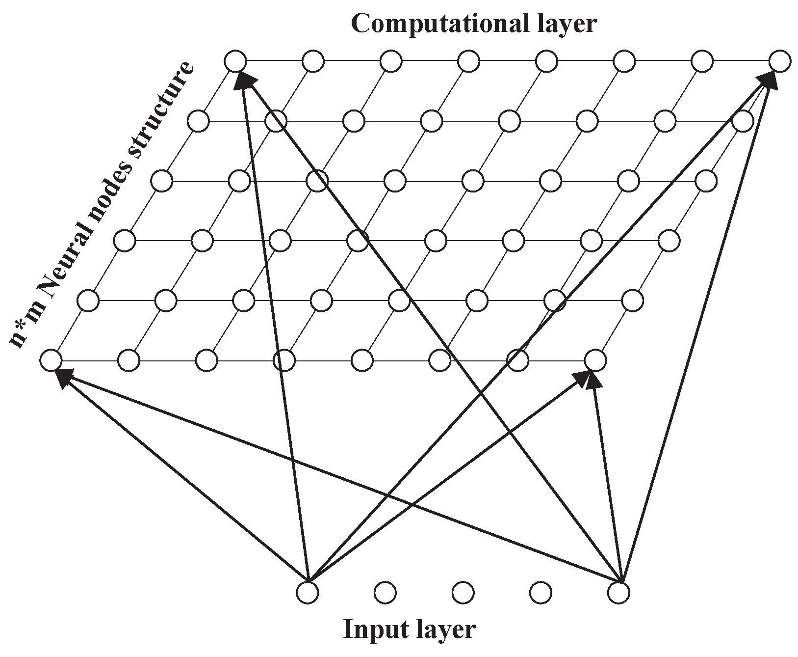
2.2. Self Organizing Maps for Clustering Time Series

As a tool for data segment, clustering is fitted to pattern recognition widely in various circumstances: mining pipeline detection, functional modules segmentation in power system, etc. [15,16]. This study attempted to explore different modules in phase space, and separate them corresponding to different countermeasures, such as the nonlinear and unpredictable intervals of a time series in real market transactions to avoid potential risks. Due to the high volatility and chaotic properties of the real financial time series data, the prediction results could be unaccountable without preprocessing, even the result turns out well-fitted [17,18,19,20,21]. In this study, the underlying financial time series data are restored in dynamics to figure out how the factors affecting price evolved. Furthermore, new factors are generated by the restoration of the time series, such as the angle matrix, which projects the linear degree into Euclidean distance for a better measurement effect.

In addition, the key moments when periodic time series convert into non-periodic time series are detected by clustering in phase space. The time sequence is projected from one dimension to a higher-dimension space after being processed by PSR. Since each dimension is related to all the other ones, the position and direction of the phase point in the space is actually determined by all of these dimensions. In fact, the reconstruction of time series is considered as a chaotic system and a differential equation system with embedded dimensions mathematically. Another problem during clustering is that for it is difficult to track the periodic transformations of the attractors, for the attractors generated by chaotic systems are entirely uncertain. What makes it worse is that it is also hard to define the period and linearity of the phase track segment of an attractor. Classical clustering algorithms—k-means, KNN, etc.—require that the number of clusters to be defined in advance [22,23,24], so the number of cycles and the degree of linearity have to be defined through assumptions first.

The nodes in SOM hidden layer are topological, and the topological relationship needs to be assumed first. In a one-dimensional model, the hidden nodes will be connected into a straight line; as to a two-dimensional topological model, the hidden nodes are connected into a plane, as shown in the Figure 2 (it is also well-known as the Kohonen network [25]):

Due to the topological property of the SOM hidden layer, an input of any dimension is capable to be discretized into one-dimensional or two-dimensional (higher dimension is rare to see) discrete space. Since the phase trajectories are of high complexity and are high-dimensional, it is also possible for SOM to carry nonlinear data by increasing the number of network layers and hidden layer nodes. Consequently, instead of defining the number of clusters, SOM is selected to map the reconstructed time series to the similar SOM neural network, and the similar phase track segments cluster in the network automatically. In Section 3.1.2, the time series data are preprocessed in order to fit the computation of SOM neural network.

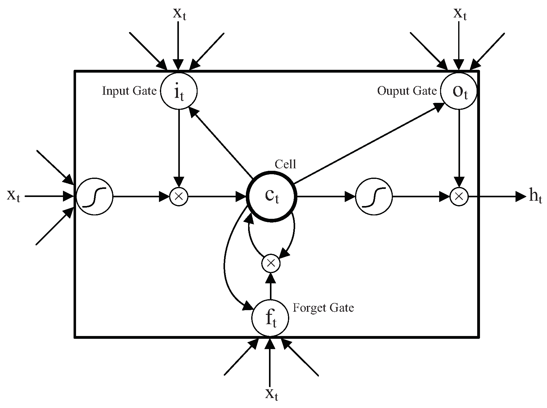
2.3. Long Short-Term Memory Model

The future data of financial time series are commonly assumed to be related to the past data, as well as the recent data and the data long ago [26]. Sepp Hochreiter and Jurgen Schmidhuber proposed the LSTM model in 1997 to predict the time series [27], and Alex Graves improved the LSTM later [28]. The LSTM unit concerns a memory cell that stores information which is updated by three special gates: the input gate, the forget gate and the output gate. LSTM unit structure is shown in Figure 3.

At time t, $t_x$ is the input data of the LSTM cell, $h_{t-1}$ is the output of the LSTM cell at the previous moment, $c_t$ is the value of the memory cell and $h_t$ is the output of the LSTM cell. The calculation process of LSTM unit can be divided into the following steps.

(1)

First, calculate the value of the candidate memory cell ${\tilde{c}}_t$; $W_c$ is the weight matrix, $b_c$ is the bias.

$${\tilde{c}}_t=tanh(W_c·[h_{t-1},x_t]+b_c)$$

(5)

(2)

Calculate the value of the input gate $i_t$. The input gate controls the updating of the current input data to the state value of the memory cell. $\sigma$ is a sigmoid function, $W_i$ is the weight matrix and $b_i$ is the bias.

$$i_t=\sigma (W_i·[h_{t-1},x_t]+b_i)$$

(6)

(3)

Calculate the value of the forget gate; the forget gate controls the updating of the historical data to the state value of the memory cell. $W_f$ is the weight matrix and $b_f$ is the bias.

$$f_t=\sigma (W_f·[h_{t-1},x_t]+b_f)$$

(7)

(4)

Calculate the value of the current moment memory cell $c_t$, and $c_{t-1}$ is the state value of the last LSTM unit.

$$c_t=f_t·c_{t-1}+i_t·{\tilde{c}}_t$$

(8)

where “.” represents dot product. The update of memory cell depends on the state value of the last cell and the candidate cell, and it is controlled by input gate and forget gate.

(5)

Calculate the value of the output gate $o_t$; the output gate controls the output of the state value of the memory cell. $W_o$ is the weight matrix and $b_o$ is the bias.

$$o_t=\sigma (W_o·[h_{t-1},x_t]+b_o)$$

(9)

(6)

Finally, calculate the output of LSTM unit $h_t$.

$$h_t=o_t·tanh\left(c_t\right)$$

(10)

LSTM retains the information of time series for a long time through three control gates and storage units. Besides, the dimension size of the output is controlled by the sharing mechanism of the LSTM internal parameters. Compared with RNN model, LSTM has a longer time delay between the input and feedback, and the error flow in memory cell is always a constant, which makes the gradient smooth and steady. Hence, it is suitable for a financial time series with a large amount of data and high volatility.

In this experiment, a 2-layer LSTM neural network structure with 100 hidden units in each layer is used to fit 1-dimensional time series, and the model is optimized by the Adam algorithm [29]. The parameter of maximum epochs is set as 1000; initial learning rate is 0.005 for every 125 iterations; the learning rate decreases by 20%; and 10% of the data are reserved for prediction. What is more, the statistical error is computed by RMSE (root mean square error), and the result of prediction is given in Section 4.

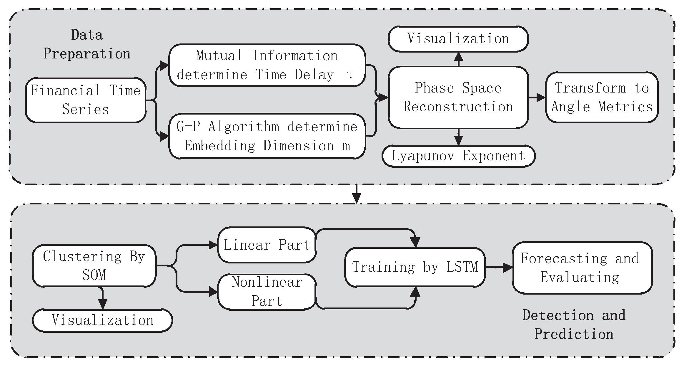
3. Technical Frameworks

Basically, the model is divided into two parts: one is data preparation and another is detection (detecting the boundary between linear and nonlinear data) and prediction. The flowchart of the model has already been given in Section 2. For the part of data preparation, the time series data are projected into a phase space, and the attractor is drawn to exhibit the dynamics in the time series directly. What is more, the Lyapunov exponent is calculated to detect the number of predictable parts of the data. Besides, data transformation is also necessary in order to adapt the data to SOM clustering. As to the detection, the phase trajectories clustered by SOM are segmented into a linear group and a non-linear group, which are verified by the supervised learning algorithm LSTM. The result shows that the segment of SOM is effective.

3.1. Data Preparation

In this study, Gold Index of China (AUL8 2013.8–2020.2), Dow Jones Industrial (DJI 1985.2–2020.2), Growth Enterprises Market Board of China (GEI 2010.6–2020.2) and Nikkei Stock Average (NIKKE225 1988.2–2020.2), are used as samples of time series.

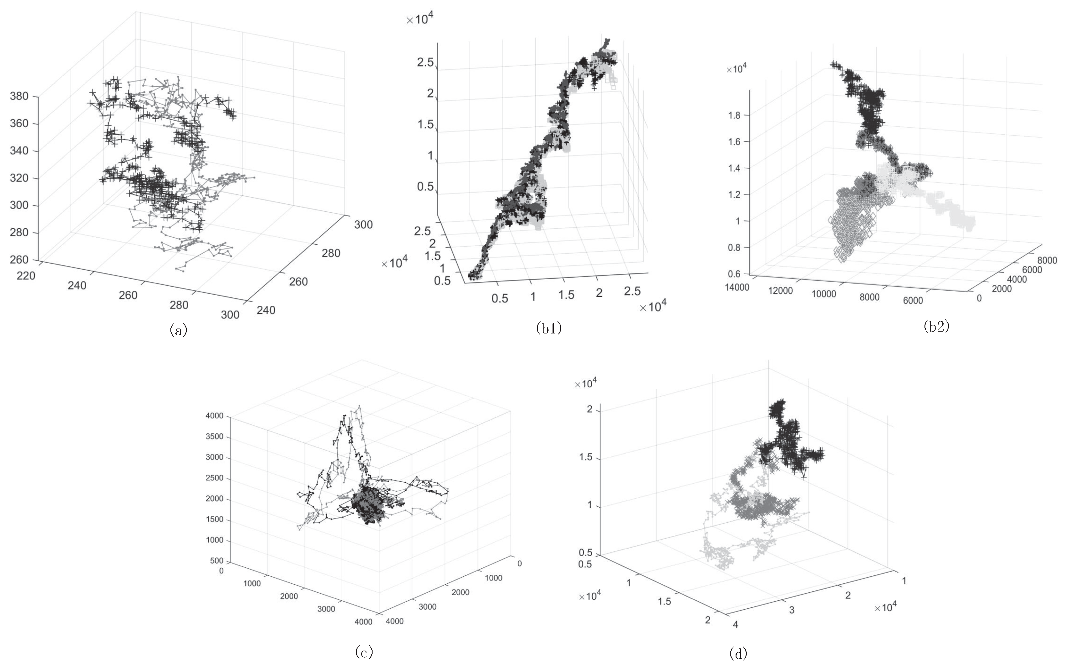
3.1.1. Phase Space Reconstruction and Visualization of Time Series Dynamics

In our previous study, nonlinear models, including an Elman neural network with time delay, a biomimetic model NBDM [4], etc., were applied to predict nonlinear financial time series, and the experiments received satisfactory prediction results. However, it is still a conundrum to predict time series in the long run. In order to solve this problem, here a new solution is proposed. Once the similar phase track segments are found in the time series, the model identifies the latest time series, and divides it into a group of clusters. In that way, the time series will repeat according to the past phase space orbit, so that it is possible to be predicted. First, the time series data are projected into a phase space to restore the phase trajectory. For example, when the fractal dimension D of a 1-dimensional time series is 1.7, since the embedded dimension should be greater than $2D+1$, here it is reasonable to take $M=5$. As to the restored data of 5-dimensional phase points, if each 1-dimensional datum with a time delay of $\tau$ is taken as a single segment, there are $n-\tau$ phase track segments in 1 dimension, and the number of track segments in the whole time series is $5(n-\tau )$. After that, the 5-dimensional data are clustered by the SOM neural network to find out the similar phase track segments. In this study, the time series data of AUL8, DJI, GEI and NIKKE225 are processed by PSR. The time delay $\tau$ of them are calculated by the mutual information algorithm, and the embedded dimension m is worked out by the G-P algorithm [30]. The Lyapunov index and average predictable step size are also calculated.

Table 1. Structural information of four datasets by PSR.

Index	Data Length N	Embeding Dimension m	Time Delay $\mathit{\tau }$	$\mathit{\tau }$_Revision	Reconstructed Structure	Lyapunov Exponent	Predictable Steps
AUL8	1574	5	649	300	5 × 374	0.0558	17.92114695
DJI	8588	10	3294	800	10 × 1388	0.0082	121.9512195
GEI	2353	8	859	200	8 × 953	0.0044	227.2727273
NIKKE225	7826	10	3503	800	10 × 626	0.0101	99.00990099

shows the construction data of the time series.

The reconstruction structure in Table 1 refers to the matrix after the transformation to phase track of time series. For example, AUL8 is transformed from a 1574 time series to 5-dimensional data with 374 data points in each dimension. Besides, the positive value of Lyapunov index indicates that it is a chaotic time series with a predictable step size of 17, which means the error will increase exponentially after 17 steps. The result is also consistent with the prediction result in Section 3.2.2.

Meanwhile, as an overly large value of $\tau$ always leads to a failure of PSR performance, it is necessary to reduce $\tau$ appropriately to continue the transformation. On the other hand, the time series cannot be expanded normally in the phase space and the dynamics of time series cannot be displayed if $\tau$ is too small, such as in a building which failed DJI, Figure 4b1. Instead of $\tau$, ${\tau }_{revision}$ is calculated and the trajectory of time series in the phase space is drawn. The result is exhibited in Figure 4a–d.

3.1.2. Generating Angle Metrics

Despite increasing the numbers of hidden layers and neural nodes to adapt high-dimensional phase trajectory, SOM is employed to identify the linear and nonlinear parts of time series. For a more precise clustering result, further data preprocessing is necessary before the clustering experiment.

For each embedding dimension, the reconstructed phase trajectory is divided into several parts with a time delay of 3, and every second point is taken as the vertex, so the angle of the three points is calculated as $\theta$. It is believed that the closer $\theta$ is to ${180}^{\circ }$, the closer the segment is to linearity, and vice versa. For example, the structure of AUL8 changes from 5 × 374 to 5 × 124, which describes 5-dimensional data with 124 angles in each dimension.

As it is known that a linear equation is still linear after superposing another linear equation, if there are linear segments of n-dimension (total m-dimension) in a same phase trajectory, the time series in the common interval with the linear segments is also linear. Figure 5a–d shows that it is rare to have $80\%$ linear region at the same time in a phase point. Meanwhile, the included angle matrix extracts the linear degree from the original phase trajectory matrix as a new influential factor, and SOM clustering is conducted to solve the problems above.

3.2. Detection and Prediction

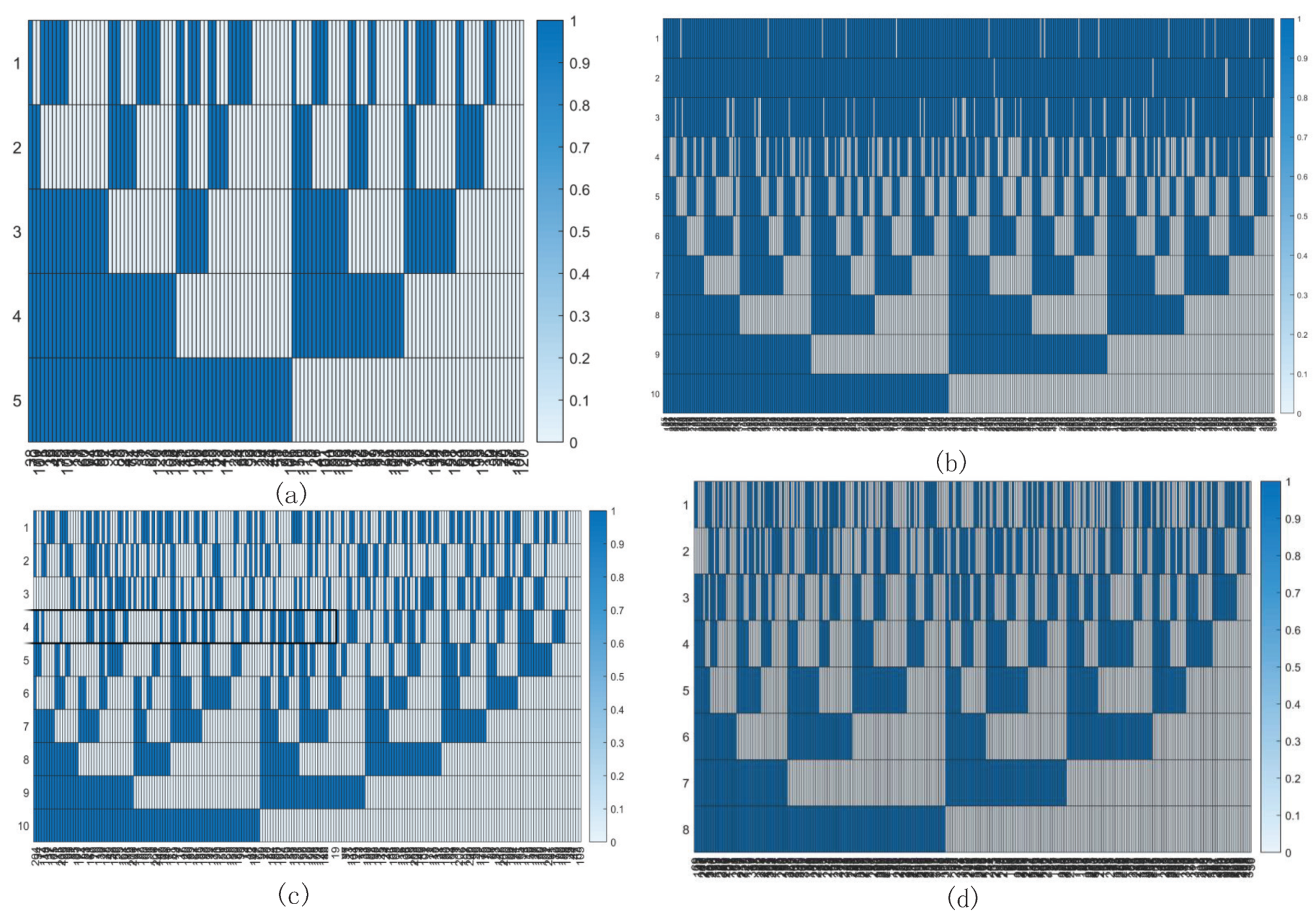
3.2.1. Detecting the Boundary between Linear and Nonlinear by SOM

After being reconstructed by the angle matrix, the datasets of the included angles are clustered by SOM. The boundary between linear and nonlinear data is able to be found when the data are divided into a low linear group and a high linear group. As the initialization of SOM, a 10 × 10 neural node structure was chosen. Before the verification of the supervised learning, whether the structure of SOM is suitable for the track segment in phase space is hard to be decided. In fact, the raw data in the experiment are only a part of the whole system, and the hypothesis is difficult to be determined. Therefore, the decision of the hypothesis itself means that the data is already predicted subjectively, by which a 10 × 10 network structure is chosen as the clustering initially. The phase track is considered linear when the phase track segment of a time series falls into the linear group mostly, which indicates that the time series is able to be predicted and vice versa. As a result, the SOM neighbor weight distances (NWD) diagram is exhibited in Figure 6a–d, from which the weights that connect each input to each of the neurons are observed intuitively. The darker the color is, the larger the weight is. If the connection patterns of two inputs are similar enough, the inputs are regarded as highly correlated.

In addition, the cluster boundary of four kinds of linear and nonlinear time series segmentation are computed and given in

Table 2. Clustering segment boundary and the division of trend to linear or nonlinear regions.

Index	Clustering Boundary	Total Linear Part Percent	80 % Linear Region	80% Nonlinear Region
AUL8	138	49.90%	t1219–t1455	t75–t632
DJI	138	45%	t1–t3448	t5060–t6996
GEI	135	44%	t197–t608	t1114–t2264
NIKKE225	145	45.70%	t139–t285	t5179–t6986

.

In the time series of AUL8, the boundary of cluster is computed as ${138}^{\circ }$, which indicates that when the included angle is greater than ${138}^{\circ }$, it is classified to the linear group by SOM, or else it should be classified to the nonlinear group; so are the other three time series. The linear group is marked as 1 and the nonlinear group as 0, and the sorted result is pictured in Figure 5a–d. It is a fact that linear phase tracking is seldom seen in a certain section. As the increasing time delay of the phase track, the linear section is even more difficult to find, and this is why the real-time financial time series is so hard to be predicted. Besides, the data close to ${180}^{\circ }$ account for $49.9\%$ in the AUL8; $80\%$ of the linear data 1219–1455, and nonlinear data 75–632 are selected to be predicted with LSTM in the next part. The calculated predictable parts of time series are not limited to seasonal changes or any one-way trend.

Furthermore, the clustering result also indicates that during the operation of the reconstructed dynamic system, the m-dimensional time series gradually carries out a transition from the linear group to the nonlinear group, and the phase trajectory deviates from the original operation trajectory. Practically, the paroxysmal chaos is an explanation of the sharp falls and rises in a real-time financial market.

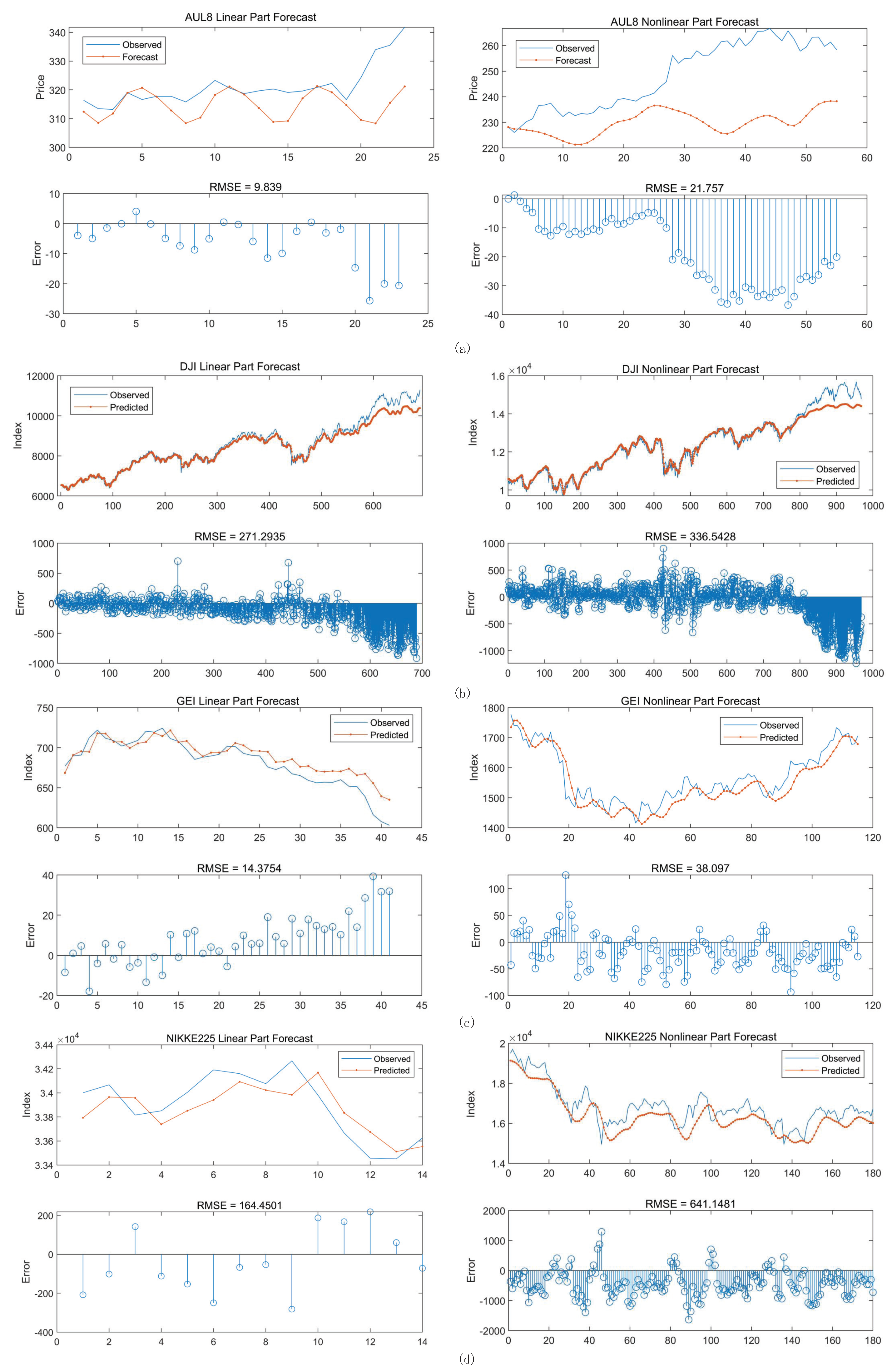
3.2.2. Predicting and Evaluating by LSTM Neural Network

After being divided into a linear group and a nonlinear group by clustering, the two groups of time series are predicted by LSTM neural network to verify the difference between them. The results of prediction are exhibited in

Table 3. Performances of different groups of four time series.

Index	AUL8 (Linear/Nonlinear)	DJI (Linear/Nonlinear)	GEI (Linear/Nonlinear)	NIKKE225 (Linear/Nonlinear)
RMSE	9.839/21.76	271.3/336.5	14.37/38.1	164.5/641.1
MAPE	1.069%/1.275%	1.190%/3.184%	1.565%/1.870%	0.7139%/3.337%
R2	99.98%/99.97%	99.98%/99.79%	99.95%/99.94%	99.98%/99.77%

by an operation of 1000 iterations in 100 times. What can be read from the table is that the predictive performance of the nonlinear group is inferior to that of the linear part, and predicting the nonlinear group of NIKKE225 is the most difficult part. Besides, the predicting performances of the two groups of DJI are close to each other, which is also reflected in Figure 5b. The linear part of DJI takes up comparatively a large area.

A more detailed forecast chart is given as Figure 7, from which the trend of error during the process of predicting is observed.

Obviously, as the non-linear prediction of the time series goes further, the error increases continuously, which corroborates the positive Lyapunov index in Table 1. That is to say, even a negligible error in the original system rises the error exponentially after a certain number of iterations, and this is why the time series in the chaotic system cannot be predicted a long time into the future. Moreover, the method of time series segmentation by SOM is effective for prediction by conducting the LSTM neural network.

4. Discussion

In this study, the four time series datasets were divided into a linear group and a nonlinear group by SOM and predicted by LSTM. It is proven that although the linear part of the time series tends to be more suitable for prediction, the boundary between the linear group and nonlinear group is not $100\%$ accurate. The difference between the restored dynamic system and the original dynamic system of the financial market is caused by the error after putting PSR on to the time series, and the error is inevitable. Therefore, the long-term prediction is reliable only when the dynamic system of the time series does not evolve for a long time in the future.

In fact, there are plenty factors affecting the dynamic system of the financial time series, such as the macro-control, natural disasters, sabotage, etc. The external influence may also stimulate the dynamic system to generate new rules and affect the time series in turn. In addition, it is the initial values which affect the operation of the time series in a chaotic system. As the phase space is regarded as a huge vector field which evolves periodically around the attractor in a price range, the dynamic reconstruction is always in the price scale. Once the price deviates from the attractor, it may break away into a space without dissipative structure, in Brownian motion. However, if paroxysmal chaos does not happen and the price runs periodically in a long time, it is thought that the price has operated in a state space which is deviated from the strange attractor. Thus, the supply and demand of the financial product is stable and the predicting result is more convincing. Although the error is inevitable and the model is not flawless, in fact, the price is not necessary to be totally predictable, and the trade does not happen in the whole process. Based on the experimental result, once the linear part of the time series is computed, it is much more possible that the transaction makes a profit. For example, if common linear segments (the value of N dimension is 0 in a column, and N accounts for $80\%$ of M in Figure 5) do not appear or a linear component is rare in the multidimensional space, the trade will not conducted until there are common linear segments detected. Therefore, the trading risk is lower and the frequency of quantitative trading operations is reduced to achieve a more accurate trading strategy.

5. Conclusions

It was concluded from the study that time series predictions achieve better results in periodic data, and a chaotic system is difficult to predict because of the sensitivity of initial values. Nowadays, there are many methods encompassing machine learning and artificial intelligence being applied to predict time series and approximate in a short time. However, the prediction results are often accompanied with over-fitting, and they can hardly provide useful guidance in real-time market trading. Therefore, the focus of this study is on analyzing the different trajectories in the clustered phase trajectories to detect the predictable part of the time series. In the experiment of the study, SOM was applied to segment the time series into two groups, a linear group and a nonlinear group. Once the phase trajectory runs into the linear group, the operation is predictable. Although it is difficult to find an absolute linear trajectory—even an $80\%$ linear trajectory is rare, and there are still errors in the prediction by the LSTM model—the unpredictable interval is able to be detected. By terminating the transaction right in time to avoid risks, the experiment is a positive for the analysis of financial time series.

References

1. Cao, J.; Li, Z.; Li, J. Financial time series forecasting model based on CEEMDAN and LSTM. Phys. A Stat. Mech. Appl. 2019, 519, 127–139. [Google Scholar] [CrossRef]
2. Wang, J.Q.; Du, Y.; Wang, J. LSTM based long-term energy consumption prediction with periodicity. Energy 2020, 197, 117197. [Google Scholar] [CrossRef]
3. Shen, Z.; Zhang, Y.; Lu, J.; Xu, J.; Xiao, G. A novel time series forecasting model with deep learning. Neurocomputing 2019. [Google Scholar] [CrossRef]
4. Zhou, T.; Gao, S.; Wang, J.; Chu, C.; Todo, Y.; Tang, Z. Financial time series prediction using a dendritic neuron model. Knowl. Based Syst. 2016, 105, 214–224. [Google Scholar] [CrossRef]
5. Lahmiri, S.; Bekiros, S. Chaos, randomness and multi-fractality in Bitcoin market. Chaos Solitons Fractals 2018, 106, 28–34. [Google Scholar] [CrossRef]
6. Kristoufek, L. Fractal markets hypothesis and the global financial crisis: Scaling, investment horizons and liquidity. Adv. Complex Syst. 2012, 15, 1250065. [Google Scholar] [CrossRef] [Green Version]
7. Wolf, A.; Swift, J.B.; Swinney, H.L.; Vastano, J.A. Determining Lyapunov exponents from a time series. Phys. D Nonlinear Phenom. 1985, 16, 285–317. [Google Scholar] [CrossRef] [Green Version]
8. Bianchi, F. The great depression and the great recession: A view from financial markets. J. Monet. Econ. 2019. [Google Scholar] [CrossRef]
9. Takens, F. Detecting Strange Attractors in Turbulence; Springer: Berlin, Germany, 1981; pp. 366–381. [Google Scholar]
10. Grassberger, P.; Procaccia, I. Estimation of the Kolmogorov entropy from a chaotic signal. Phys. Rev. A 1983, 28, 2591. [Google Scholar] [CrossRef] [Green Version]
11. Zhiqiang, G.; Huaiqing, W.; Quan, L. Financial time series forecasting using LPP and SVM optimized by PSO. Soft Comput. 2013, 17, 805–818. [Google Scholar] [CrossRef]
12. Zhang, L.; Tian, F.; Liu, S.; Dang, L.; Peng, X.; Yin, X. Chaotic time series prediction of E-nose sensor drift in embedded phase space. Sens. Actuators B Chem. 2013, 182, 71–79. [Google Scholar] [CrossRef]
13. Fan, X.; Li, S.; Tian, L. Chaotic characteristic identification for carbon price and an multi-layer perceptron network prediction model. Expert Syst. Appl. 2015, 42, 3945–3952. [Google Scholar] [CrossRef]
14. Shang, P.; Na, X.; Kamae, S. Chaotic analysis of time series in the sediment transport phenomenon. Chaos Solitons Fractals 2009, 41, 368–379. [Google Scholar] [CrossRef]
15. Ghadiri, S.M.E.; Mazlumi, K. Adaptive protection scheme for microgrids based on SOM clustering technique. Appl. Soft Comput. 2020, 88, 106062. [Google Scholar] [CrossRef]
16. Teichgraeber, H.; Brandt, A.R. Clustering methods to find representative periods for the optimization of energy systems: An initial framework and comparison. Appl. Energy 2019, 239, 1283–1293. [Google Scholar] [CrossRef]
17. Dose, C.; Cincotti, S. Clustering of financial time series with application to index and enhanced index tracking portfolio. Phys. A Stat. Mech. Appl. 2005, 355, 145–151. [Google Scholar] [CrossRef]
18. Niu, H.; Wang, J. Volatility clustering and long memory of financial time series and financial price model. Digit. Signal Process. 2013, 23, 489–498. [Google Scholar] [CrossRef]
19. Pattarin, F.; Paterlini, S.; Minerva, T. Clustering financial time series: An application to mutual funds style analysis. Comput. Stat. Data Anal. 2004, 47, 353–372. [Google Scholar] [CrossRef]
20. Dias, J.G.; Vermunt, J.K.; Ramos, S. Clustering financial time series: New insights from an extended hidden Markov model. Eur. J. Oper. Res. 2015, 243, 852–864. [Google Scholar] [CrossRef] [Green Version]
21. Nie, C.X. Dynamics of cluster structure in financial correlation matrix. Chaos Solitons Fractals 2017, 104, 835–840. [Google Scholar] [CrossRef]
22. Liu, G.; Zhu, L.; Wu, X.; Wang, J. Time series clustering and physical implication for photovoltaic array systems with unknown working conditions. Sol. Energy 2019, 180, 401–411. [Google Scholar] [CrossRef]
23. Li, H. Multivariate time series clustering based on common principal component analysis. Neurocomputing 2019, 349, 239–247. [Google Scholar] [CrossRef]
24. Song, X.; Shi, M.; Wu, J.; Sun, W. A new fuzzy c-means clustering-based time series segmentation approach and its application on tunnel boring machine analysis. Mech. Syst. Signal Process. 2019, 133, 106279. [Google Scholar] [CrossRef]
25. Kohonen, T. The self-organizing map. Proc. IEEE 1990, 78, 1464–1480. [Google Scholar] [CrossRef]
26. Bengio, Y.; Simard, P.; Frasconi, P. Learning long-term dependencies with gradient descent is difficult. IEEE Trans. Neural Netw. 1994, 5, 157–166. [Google Scholar] [CrossRef] [PubMed]
27. Hochreiter, S.; Schmidhuber, J. Long short-term memory. Neural Comput. 1997, 9, 1735–1780. [Google Scholar] [CrossRef]
28. Graves, A. Generating sequences with recurrent neural networks. arXiv 2013, arXiv:1308.0850. [Google Scholar]
29. Kingma, D.P.; Ba, J. Adam: A Method for Stochastic Optimization. arXiv 2014, arXiv:1412.6980. [Google Scholar]
30. Fraser, A.M.; Swinney, H.L. Independent coordinates for strange attractors from mutual information. Phys. Rev. A 1986, 33, 1134–1140. [Google Scholar] [CrossRef]
Figure 1. The proposed methodological flowchart.
Electronics 09 00823 g001
Figure 2. Typical SOM neural network structure.
Electronics 09 00823 g002
Figure 3. Architecture of the memory block of LSTM.
Electronics 09 00823 g003
Figure 4. Attractor of four datasets: (a) AUL8, (b1) DJI with an unsuitable time delay τ , (b2) DJI, (c) GEI and (d) NIKKE225 in the phase space.
Electronics 09 00823 g004
Figure 5. Visualization of linear group (marked as 1) in each embedding dimension with a sorting. (a) AUL8, (b) DJI, (c) GEI and (d) NIKKE225.
Electronics 09 00823 g005
Figure 6. SOM neighbor weight distances for four datasets: (a) AUL8, (b) DJI, (c) GEI and (d) NIKKE225.
Electronics 09 00823 g006
Figure 7. Four time series (a) AUL8, (b) DJI, (c) GEI and (d) NIKKE225. predictions with different groups (trend to linear part or trend to nonlinear part), and the RMSE in every small forecast step.
Electronics 09 00823 g007