Article

Validation of Large-Scale Classification Problem in Dendritic Neuron Model Using Particle Antagonism Mechanism

1
School of Computer Engineering, Jiangsu Ocean University, Lianyungang 222005, China
2
Department of Management, eSOL Co., Ltd., Tokyo 164-8721, Japan
3
Faculty of Electrical, Information and Communication Engineering, Kanazawa University, Kanazawa-shi 920-1192, Japan
*
Author to whom correspondence should be addressed.
Electronics 2020, 9(5), 792; https://doi.org/10.3390/electronics9050792
Submission received: 15 April 2020 / Revised: 27 April 2020 / Accepted: 1 May 2020 / Published: 11 May 2020
(This article belongs to the Special Issue Applications of Bioinspired Neural Network)

Abstract

:
With the characteristics of simple structure and low cost, the dendritic neuron model (DNM) is used as a neuron model to solve complex problems such as nonlinear problems for achieving high-precision models. Although the DNM obtains higher accuracy and effectiveness than the middle layer of the multilayer perceptron in small-scale classification problems, there are no examples that apply it to large-scale classification problems. To achieve better performance for solving practical problems, an approximate Newton-type method-neural network with random weights for the comparison; and three learning algorithms including back-propagation (BP), biogeography-based optimization (BBO), and a competitive swarm optimizer (CSO) are used in the DNM in this experiment. Moreover, three classification problems are solved by using the above learning algorithms to verify their precision and effectiveness in large-scale classification problems. As a consequence, in the case of execution time, DNM + BP is the optimum; DNM + CSO is the best in terms of both accuracy stability and execution time; and considering the stability of comprehensive performance and the convergence rate, DNM + BBO is a wise choice.

Graphical Abstract

1. Introduction

Along with the arrival of the era of big data, the third wave of artificial intelligence (AI) has been entered [1]. AI is being advanced for uniting IoT and robotics, not just as a research craze but through technological advances in hardware.
Commercialized AI is used as a system of prediction or classification that has been confirmed with high precision [2]. In general, it is difficult and indispensable to classify high quality data from vast amounts of data that contain all the information. However, if the problem is solved using AI, the cost can be greatly reduced. Moreover, the classification problems also exist in fields other than AI [3,4,5]. For example, in the field of gamma ray research in astronomy, cosmic rays can be observed through a telescope [6]. Due to the complexity of radiation, measurements are currently made using Monte-Carlo simulation. The ability to classify and detect gamma rays based on a limited set of characteristics would contribute to further improvements in telescopy.
The neural network is a symbolic presence that can deal with nonlinear problems in the third wave of AI [7,8]. In particular, with the deep learning of the middle layer of the multilayer perceptron (MLP) [9,10], which uses nonlinear functions to network, the accuracy is improved with an increase in the amount of data used for learning. However, as the deepening of middle layer and the number of processed data increase, the computing cost becomes huge. As a consequence, with the characteristics of simple structure and cost saving, research into the dendritic neuron model (DNM) [11,12,13,14,15,16] is being developed to achieve high-precision models. Unlike other neural networks, the DNM is a model of one neuron, and much research indicates that the DNM has better performance than the MLP in small-scale classification problems [17,18]. Additionally, it is proved that the model, with its excellent metaheuristics, can obtain better classification accuracy by the previous optimization experiment for weight and threshold for small-scale classification problems with the DNM.
In various neuronal models and neural networks, it is necessary to change the weight of bonding strength between neurons in order to reduce the error in the desired output. However, as the neural network with random weights (NNRW) cannot guarantee the convergence of errors to the desired output, it is not considered to be a practical learning algorithm [19,20].
Generally, the learning algorithm is used to solve difficult optimization problems since the weighted learning can be considered as an optimization problem. The most famous learning algorithm in local exploration is the back-propagation (BP) [21,22,23], which computes the gradient using the chain rule and has the advantage of low learning cost since the installation is simple. In addition, the method of multi-point exploration, which is used as a model to classify according to natural phenomena and laws, is documented [24]. For example, the gravitational search algorithm is a basic learning algorithm to simulate physical phenomena [25,26,27,28,29], biogeography-based optimization (BBO) [30] is generally used for simulating ecological concepts since the accuracy and stability are the most outstanding among the models using representative metaheuristics [31], and some basic learning algorithms can simulate the moving sample population of organisms such as particle swarm optimization (PSO) [32,33] and ant colony optimization. Moreover, as a variant of PSO, the competitive swarm optimizer (CSO) [34,35] is a simplified metaheuristics set that is suitable for both multi-point and local exploration. Compared to the systems hat only conduct multi-point exploration or local exploration, the trap of the local optimal solution and convergence rate can be balanced using the CSO.
Although the DNM has shown higher accuracy and effectiveness than the MLP in small-scale classification problems, there are no examples that apply it to large-scale classification problems [36]. In this paper, the most famous learning algorithm using a gradient descent method with low computing cost, BP; the high classification accuracy algorithm for small-scale classification problems, BBO; and the especially low cost CSO algorithm are highlighted. The DNM is applied to large-scale classification problems with the above three learning algorithms, respectively. Consequently, the learning algorithm with BP is named DNM + BP, and DNM + BBO and DNM + CSO are named in a similar way. As a comparison object, the approximate Newton-type method (ANE)-NNRW is selected since it was applied to the same classification problem in the previous study. The ANE-NNRW is an NNRW based on the forward propagation MLP that ensures the convergence of solutions by an approximate Newton-type method [37].
Therefore, this study verifies the effectiveness of the DNM for large-scale classification problems, very important information for studying the performance of DNM.

2. Model and Learning Algorithm

2.1. Dendritic Neuron Model

The DNM is a model that vests dendrite function to the existing single layer perceptron [38,39,40] and is composed of four layers. Inputs x1, x2, …, xn in each dendrite are firstly transformed to their corresponding outputs according to four connection instances in the synaptic layer, which possesses a sigmoid function for received inputs. Secondly, all the outputs from the synaptic layer in each dendrite are multiplied as new outputs of the dendrite layer. Thirdly, all the outputs in the dendrite layer are summed to obtain an output of the membrane layer. Finally, this output of the membrane layer is regarded as the input of the soma layer, which utilizes another sigmoid function to calculate the ultimate result of the DNM. The complete structure of the DNM is shown in Figure 1, and its details are described as follows.

2.1.1. Synaptic Layer

A synapse connects neurons from a dendrite to another dendrite/axon or the soma of another neural cell. The information flows from a presynaptic neuron to a postsynaptic neuron, which shows feedforward nature. The changes in the postsynaptic potential influenced by ionotropic phenomena determine the excitatory or inhibitory nature of a synapse. The description connecting the ith (i = 1, 2, …, n) synaptic input to the jth (j = 1, 2, …, m) synaptic layer is given as
  Y i j = 1 1 + e k ( w i j x i θ i j )
where Yij is the output from the ith synaptic input to the jth synaptic layer. k indicates a positive constant. xi manifests the ith input of a synapse and xi ∈ [0, 1]. Weight wij and threshold θij are the connection parameters to be learned.
According to the values of wij and θij, four types of connection instance are shown in Figure 2, where the horizontal axis indicates the inputs of presynaptic neurons and the vertical one clarifies the output of the synaptic layer. As the range of x is [0, 1], only the conforming part is required to be seen. The four connection instances contain:
Figure 2a,b presents wij < 0 < θij or 0 < wij < θij, where the output is approximately 0 no matter when the input transforms from 0 to 1;
Figure 2c,d presents θij < 0 < wij or θij < wij < 0, where the output is approximately 1 no matter when the input transforms from 0 to 1;
Figure 2e depicts 0 < θij < wij, where the output is proportional to the input no matter when the input transforms from 0 to 1;
Figure 2f depicts the inhibitory connection when wij < θij < 0, where the output is inversely proportional to the input no matter when the input transforms from 0 to 1. It is worth noting that these four connection instances are critical to infer the morphology of a neuron by specifying the positions and synapse types of dendrites.

2.1.2. Dendrite Layer

The dendrite layer shows a multiplicative function of the outputs from synapses at various synaptic layers [41]. A type of multiplicative operation can be achieved due to the nonlinearity of synapses, i.e., constant 0 or 1 connection. That is why a multiplicative operation has been chosen to use in this model when it comes to the dendrite layer. The multiplication is equivalent to the logic and operation since the values of inputs and outputs of the dendrites correspond to 1 or 0. The output function for the jth dendrite branch is expressed as follows:
Z j = i = 1 n Y i j

2.1.3. Membrane Layer

The membrane layer collects the signals from each dendritic branch. The input received from a dendrite branch is calculated with a summation function, which closely resembles a logic or operation. Then, the resultant output is delivered into the next layer to activate the soma body. The output of this layer is formulated as
V = j = 1 m Z j

2.1.4. Soma Layer

At last, the soma layer implements the function of soma body such that the neuron fires if the output from the membrane layer exceeds its threshold. This process is expressed by a sigmoid function used to calculate the ultimate output of the entire model:
O = 1 1 + e k s ( V θ s )
The parameter ks is a positive constant, and the threshold θs varies from 0 to 1.
According to the multiplication of each dendrite, the DNM can be used as a neuron model and solve complex problems such as nonlinear problems. In addition, in terms of the activation function of synaptic layer and soma layer, the sigmoid function is used in reference to previous studies.

2.2. Back-Propagation

BP is a point gradient descent learning algorithm that uses chain law to calculate the gradient [42,43]. The construction of the neuron model depends on an effective learning rule. Its learning rule is obtained by the least squared error between the real output vector O and the target output vector T, shown as follows:
E = 1 2 ( T O ) 2
The error is decreased by correcting the synaptic parameters wij and θij in the DNM of the connection function during learning. The updated equations are expressed as follows:
Δ w i j ( t ) = p = 1 P E p w i j , Δ θ i j ( t ) = p = 1 P E p θ i j
where η represents the learning rate, which is a user-defined parameter, and Ep is the mean square error. Then, the updating rules of wij and θij are computed as follows:
w i j ( t + 1 ) = w i j ( t ) η Δ w i j ( t ) , θ i j ( t + 1 ) = θ i j ( t ) η Δ θ i j ( t )
where t is the number of the learning iteration. In addition, the partial differentials of Ep with regard to wij and θij are defined as follows:
E p w i j = E p O p O p V V Z j Z j Y i j Y i j w i j ,   E p θ i j = E p O p O p V V Z j Z j Y i j Y i j θ i j
The detail parts of the above partial differentials are represented as follows:
E p O p = T p O p O p V = k s x i e k s ( w i j x i θ s ) ( 1 + e k s ( w i j x i θ s ) ) 2   V Z j = 1 Z j Y i j = l = 1 a n d l i n Y l j   Y i j w i j = k x i e k ( w i j x i θ i j ) ( 1 + e k ( w i j x i θ i j ) ) 2   Y i j θ i j = k e k ( w i j x i θ i j ) ( 1 + e k ( w i j x i θ i j ) ) 2
In the calculation of ∆wij(t) and ∆θij(t), the partial differential is obtained from input to output in order and in reverse order.

2.3. Biogeography-Based Optimization

BBO is a metaheuristics model of the speciation, extinction, and geographical distribution in biogeography, whose characteristic takes the habitat as a solution and shares the suitability index variables (SIVs) with other habitats directly [44]. The fitness values of other learning algorithms are expressed as the habitat suitability index (HSI), implemented as follows:
  • Current rank of habitat Hi (i = 1, 2, …, n) produces the integer spectrum SIV.
  • The HSI of each habitat is calculated using the following equation:
    H S I ( H i ) = 1 2 P p = 1 P ( T p O p ) 2
    where P is the total number of training samples, Tp is the target vector of the pth sample, and Op is the actual output vector obtained by Hi.
  • The SIV is randomly selected and immigration to other habitats occurs according to the calculations of the emigration rate μi and immigration rate λi.
    μ i = E i m λ i = I ( 1 i m )
    where E is the emigration rate, and I is the maximum immigration rate. The case that E = I = 1 is considered in BBO, and the relationship between λ and μ is established as the following formula:
    λ i + μ i = E
  • For each habitat Hi, the immigrated HSI and the probability, Psi, that it contains the Sth species of habitat are updated.
    P s i ( t + Δ t ) = P s i ( t ) ( 1 λ i Δ t μ i Δ t ) + P s i 1 λ i 1 Δ t + P s i + 1 μ i + 1 Δ t
    If t is sufficiently small, the following equation can be approximated:
    P s i = { ( λ i + μ i ) P s i + μ i + 1 P s i + 1                                           i = 0 ( λ i + μ i ) P s i + λ i 1 P s i 1 + μ i + 1 P s i + 1         1 i n 1 ( λ i + μ i ) P s i + λ i 1 P s i 1                                           i = n
  • Species numbers are varied according to the mutation rate, Pmi, for non-elite habitats:
    P m i = P m m a x 1 P s i P s m a x
    where Psmax is the maximum value of Psi, and Pmmax is the parameter.
  • Step 2 is returned to for the next iteration. The algorithm does not end until the termination condition is satisfied.

2.4. Competitive Swarm Optimizer

The CSO is a kind of group intelligence that improves PSO to face large-scale classification problems. It is a mechanism for comparing the evaluation results of different particles selected from the population; only the failed particles are learned to update [45]. Therefore, in addition to the number of updated particles being able to be reduced to 2/N, the excellent solutions in the search do not need to be saved, and it can be used for efficient search on large-scale classification problems. As with PSO, the individual movement with speed will not be eliminated. The operating steps are shown as follows:
  • For N initial solutions, the particle position xi(i = 1, 2, …, N) and velocity vi(i = 1, 2, …, N) of generated particles are calculated.
  • All solutions are evaluated.
  • The kth (k = 1, 2, …, 2/N) competition for generation t occurs as follows:
    (a)
    The non-repeating particles Nk1 and Nk2 are randomly selected from the undecided particles.
    (b)
    The positions of selected particles of Nk1 and Nk2 are compared and evaluated to determine the winning particle and the failing particle.
    (c)
    A velocity vl,k is applied to the position xl,k of the failed particle to make it move.
    v l , k ( t + 1 ) = R 1 ( k , t ) v l , k ( t ) + R 2 ( k , t ) [ x w , k ( t ) x l , k ( t ) ] + φ R 3 ( k , t ) [ x k ¯ ( t ) x l , k ( t ) ] ,   x l , k ( t + 1 ) = x l , k ( t ) + v l , k ( t + 1 )
    where R1(k, t), R2(k, t), and R3(k, t) are the random vectors of [0, 1], x k ¯ ( t ) is the average position of the whole particles, and φ is the control parameter that sets the degree of influence from the average position, which is recommended as the following conditions in the previous study:
    { φ = 0                                                                           N 100 φ [ 0.14 log ( N ) 0.3 ,   0.27 log ( N ) 0.51 ]         o t h e r w i s e
    (d)
    Operations (a) through (c) are repeated until all the particles are decided.
  • Step 2 is returned to for the next iteration. The algorithm does not end until the termination condition is satisfied.

3. Experiment

Three classification problems in our experiments are shown in Table 1 below. The most downloaded open data sets in different fields of the UCI Machine Learning Repository are used [46], and the value of the characteristic number does not contain the class. F1 classifies whether the cosmic ray received by the Cherenkov telescope is a gamma ray or not, F2 classifies whether the space shuttle radiator is abnormal, and F3 classifies whether the pixel is skin based on the RGB information of the image. Furthermore, the characteristics of any classification problem are expressed by numbers with no data error that contain negative numbers and decimal numbers. According to the input range of the synaptic layer, each characteristic data set is standardized for the experiment.
Each classification problem is tested 30 times independently, and the accuracy of the expected output is calculated according to the classification results. The formula of accuracy is shown in the Equation (18) with TP (true positivity), FP (false positive), TN (true negative), and FN (false negative).
a c c u r a c y = T P + T N T P + F P + T N + F N × 100 %
Besides, the mean square error (MSE) is determined as the evaluation function of the solution that is obtained through Equation (5) for DNM + BP, and Equation (19) for DNM + BBO and DNM + CSO:
M S E = 1 2 P p = 1 P ( O p T p ) 2
The termination condition is set to reach the maximum generation number; for DNM + BP, it is 1000; and for DNM+BBO and DNM + CSO, it is 200, according to the ANE-NNRW. The population number of BBO and CSO is 50.
In addition to the partition ratio of F2, which is specified by the data set, the learning data account for 70% and the testing data account for 30%, referring to the previous study of the DNM as shown in Table 2 [18], and the proportion in the ANE-NNRW is shown in Table 3. In order to make the dimensions consistent, the maximum value of m is set based on the maximum value of m of the interlayer in the previous study.
Moreover, considering the processing load of the DNM, the upper limit of m is 100. Table 4 shows a list of m for the previous study and dimension D and m for this study. Due to the experimental load and time, F1, F2, and F3 use different environments as shown in Table 5.
According to the design of experiment, which is a statistical method for the effective analysis of large combinations using orthogonal arrays based on Latin square, DNM + BP, DNM + BBO, and DNM + CSO are conducted under the above conditions, and the number of experiments can be greatly reduced by the relationship between the factors and levels.
Each factor and level will be applied in the orthogonal array of L25 (56) since this experiment has five factors and five levels. Table 6 and Table 7 represent lists of factors and levels used in F1, F2, and F3.
Table 8 applies to the parameters of F1, and Table 9 applies to those of F2 and F3. Moreover, the numbers in Table 8 and Table 9 are the combination numbers of the experimental parameters.

4. Results

By calculating the average accuracy, the optimum parameters used in this experiment are selected as shown in Table 10, Table 11 and Table 12, respectively.
The average accuracy and standard deviation of each problem and learning algorithm are shown in Table 13. It is clearly that DNM + BP in F1, DNM + CSO in F2, and DNM + BBO in F3 have the highest accuracy.
The results of the ANE-NNRW as the comparison object are shown in Table 14, and the accuracy of the previous paper is recorded as a percentage [19]. Obviously, the accuracy of the DNM is higher than that of the ANE-NNRW in all problems. They also prove that the DNM has the advantage of high accuracy even if the data required for learning are not as much as for the ANE-NNRW, which corresponds to Table 2 and Table 3.
Table 15 summarizes the average execution time and optimum parameter m, which is in deep relation to dimension D. The execution time of the DNM is larger than that of the ANE-NNRW as shown in Table 15 [19].
Even in DNM + BP, which has the lowest computational cost in the experimental method, the execution time of the 200th generation is at least four times that of the ANE-NNRW. One of the reasons for this is that the DNM is more time-consuming than the MLP, which is also mentioned in the case of small-scale classification problems. Additionally, the ANE-NNRW is a calculation method based on the pure propagation MLP; it is considered that a similar result should appear for this large-scale classification problem. Secondly, the ANE-NNRW is an efficient way to solve the large-scale problem; the data set segmentation is performed. Besides, the computational cost is less by learning with random weighting to ensure convergence.
According to the average execution time of DNM+BBO and DNM + CSO in F2 and F3, as the optimum parameter m of DNM + BBO is higher than that of DNM + CSO, there is a large difference of more than 3000 seconds between the two methods in F2. Similarly, because the value of m is the same in F3, the difference is about 10 seconds since DNM + BBO has more order of solution updates. In addition, the difference between DNM + BBO and DNM + CSO in F1 can also be considered as the difference between m, but it is not as great as in F2. Therefore, DNM+CSO is better than DNM + BBO in terms of the execution time of the learning algorithm.
On the other hand, for DNM + BP and DNM + CSO, there is a difference of at least 1000 seconds in the execution time between F1 and F2 under the same m, which is caused by the difference in the number of data and features.
As the DNM calculates m and the number of features using Equation (1), it is confirmed that the execution time approximately follows the calculated amount for the model. Consequently, the execution time increases due to the increase in the number of data. In the same problem, it is desirable that a smaller value of m can reduce the time. However, the m of DNM + BP in F2 and F3 obviously shows that the difference in execution time cannot be determined by the number of data alone.
Therefore, for improving the precision, it is necessary to set an upper limit, split data, and process in parallel to reduce the load of a large-scale problem since the DNM varies in precision according to the set parameters.
Furthermore, the upper limit of m is set as 100 in this experiment, but both of the optimum parameters m of DNM + BBO and DNM + CSO in F3 are 50, half of the upper limit, with a high accuracy of classification as shown in Table 13. Therefore, for large-scale classification problems, DNM learning by metaheuristics may not require an extremely large number of m for problems with a small number of features. As a reference for parameter determination in the application of the DNM to large-scale problems, this will be clarified in the future.
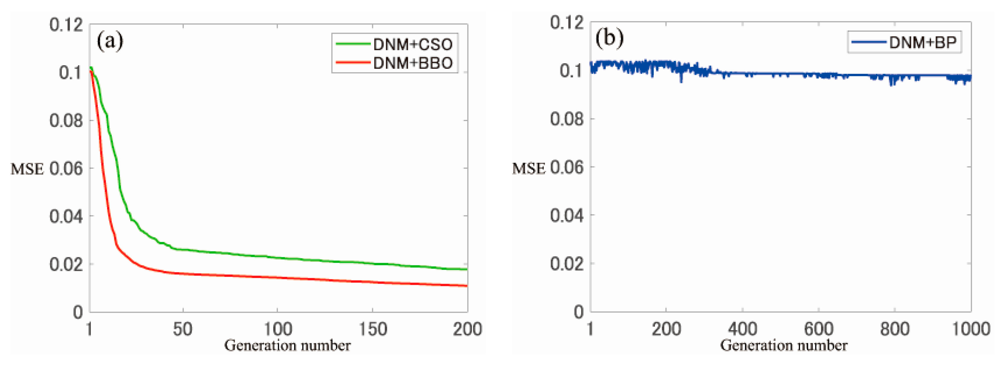
The average convergence graph of each generation of MSE obtained by experiments are shown in Figure 3, Figure 4 and Figure 5. Figure 3a presents the DNM + BBO and DNM + CSO convergence graphs of F1, and Figure 3b presents the DNM + BP convergence graph of F1. In a similar way, the convergence graphs of F2 and F3 are shown in Figure 4 and Figure 5, respectively.
It is clearly that the values of each learning algorithm converge to the end generation number and that DNM + BBO converged first in all cases. In order to reduce the computation, the CSO only updates the solution of particles equal to half of the population numbers. The BBO of the same multi-point search keeps the elite habitat and changes the solution in each generation, and the number of new candidate optimum solutions produced in one generation is larger than that with the CSO. As a new solution is derived from a candidate optimum solution at a certain point in time, the convergence rate of the higher quality solution will be accelerated. Therefore, it is considered that BBO is more suitable than the CSO to obtain a small MSE with a smaller number of generations.
Furthermore, the MSE does not change greatly due to the local solution of F3 in Figure 5b, indicating that BP with a feature that tends to trapped in the local solution has the shortcoming of the problem orientation not being significant compared with that with the multi-point search method, with which it is easy to escape from the local solution.
The stability of each method in F1, F2, and F3 is illustrated by the box-plots of Figure 6, Figure 7 and Figure 8, respectively. In the case of the minimum MSE of each problem, F1 is DNM + CSO, and F2 and F3 are DNM + BBO. Besides, for the maximum MSE of each problem, F1 is DNM + BBO, and F2 and F3 are DNM + BP.
However, for the comprehensive consideration, it can be seen that DNM + BP in F1, DNM + CSO in F2, and DNM + BBO in F3 record the best stability. Moreover, the average values of MSE for the end conditions in each problem and method are shown in Table 16. It shows that the method with excellent stability in each problem is also superior to other methods in terms of the average MSE.
Furthermore, the average of standard deviation of accuracy and the standard deviation of each method for the tests are shown in Table 17 below. Although DNM + BP has the best stability in F1, both the average value and standard deviation are the highest, which indicates that DNM + BP has a large deviation according to the different problems. To the contrary, DNM + BBO and DNM + CSO have more stability that is not easily affected by these three problems of this experiment.
As a consequence, in terms of the convergence and stability of MSE, it is better to adopt a multi-point search method, especially DNM + BBO with the advantage in terms of the convergence rate.
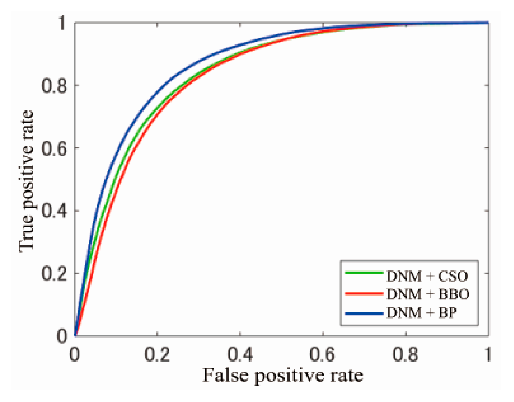
Figure 9, Figure 10 and Figure 11 depict the receiver operating characteristic (ROC) of each method in F1, F2 and F3, respectively. Furthermore, the average value of area under curve (AUC) in each problem and method is shown in Table 18.
According to Figure 9 and Figure 11, DNM + BP in F1 and DNM + BBO in F3 obtain the highest classification accuracies. On the other hand, the three methods overlap on the diagonal line in Figure 10, and the results are similar to those in the case of random classification since the value of AUC is very close to 0.5, as shown in Table 18.
Although DNM + BBO and DNM + CSO differ to some degree in Figure 9 and Figure 11, both of them are convex curves to the upper left. In particular, the AUC of F3 is close to 1, which shows that their classification accuracy is excellent. However, for DNM + BP, the best AUC is a convex curve to the upper left in F1, while F3 is a curve that approximates the diagonal.
On the other hand, in Table 13 and Table 18, the difference in accuracy between DNM + BBO and DNM + CSO in F1 and F3 is also reflected in the AUC. To the contrary, even though the difference in accuracy of DNM + BP in F1 and F3 is only about 1%, the AUC is about 0.3. This is because the value of Op that outputs the error classification result contains many values independent of the set threshold value of DNM + BP in F3. As shown in Figure 5b, the DNM + BP in F3 is trapped in the local solution since it fails to obtain the output with a higher classification accuracy.
As DNM + BP in F3 above, the value of Op that outputs the error classification result contains many values independent of the set threshold value as shown in Figure 10, and the results are almost arranged on the same diagonal by any method in F2. The data set is considered to be the reason for this.
Moreover, because the output range of the DNM is [0, 1], the upper limit of the classifiable class is 2. In this experiment, in order to classify in the DNM, all of the classes representing the abnormality of F2 are unified as a non-anomaly class. It can be seen that the output with a high classification accuracy is not available since the different data trends are aggregated in the class representing each abnormality. Therefore, depending on the network of the DNM, etc., it is possible to expand the output range of the DNM effectively for improvement.
In addition, the average rank of the methods in F1, F2, and F3 obtained by the Friedman test are shown in Table 19. It is clear that DNM + BP in F1, DNM + CSO in F2, and DNM + BBO in F3 ranked the highest on average, that there is no difference in the average accuracy for each problem, and that the result of this test is proved to be significant.

5. Discussion

According to Table A1, Table A2 and Table A3 in the appendix, Table 20 shows the standard deviation of the average accuracy of each method. It can be seen that the accuracy of DNM + BP is the most affected by the combination of the parameters in F1 and F2. In the experiment for optimum parameter selection, the stability is slightly poor. However, the result of DNM + BP in F3 shows that it is not affected by the parameters and is trapped in the local solution with stability. In addition, the average accuracy of the DNM + CSO test in F3 is 20.78% of No. 21 as shown in appendix in Table A3, which is the lowest average accuracy among all methods.
Therefore, in terms of the stability of parameters, no matter which learning algorithm is used, the accuracy will deviate according to compatibility with the problem and the combination of parameters. Due to the nature of neural networks, it is difficult to predict the accuracy deviation based on parameters and learning algorithms, so a variety of methods should be performed for the experiment.

6. Conclusions

With the arrival of the era of big data, research into high-precision models with simple structures and low cost for addressing complex problems is developing rapidly. As a neuron model, the DNM has been proven to be more accurate than the MLP in small-scale classification problems. This study focused on the application of the DNM in complex problems and verified its effectiveness in large-scale classification problems. The DNM, as the model; BP, the most famous method for using the gradient descent to calculate the cost; BBO, with a high classification accuracy for small-scale problems; and CSO, which has the characteristic of low computational cost, were used as the learning algorithms in this experiment.
The comparison results for the three large-scale classification problems with the ANE-NNRW show that any learning algorithm using the DNM can achieve a higher accuracy than the ANE-NNRW. However, they lag behind the ANE-NNRW in terms of execution time. In order to improve this situation, it is necessary to parallelize the parts of the DNM and reduce the computing cost.
Moreover, according to the applied three large-scale classification problems, the precision and classification accuracy of each DNM method are different. This experiment compared each learning algorithm in various aspects. In terms of execution time, DNM + BP is the optimum; DNM + CSO is the best to ensure both accuracy stability and short execution time; and considering the stability of comprehensive performance and convergence rate, DNM + BBO is a wise choice. In the future, for seeking stability independent of the problem, we will attempt to expand the output range of the DNM and employ it across a wider range of fields, e.g., Internet of Vehicles [47,48,49,50] and complex networks [51,52,53]. In addition, recent advanced evolutionary algorithms, e.g., chaotic differential evolution [54], can also be an alternative training method for the DNM.

Author Contributions

Conceptualization, D.J., C.L., Y.T. and H.D.; Data curation, D.J. and Y.F.; Formal analysis, C.L. and H.D.; Funding acquisition, D.J., C.L., Y.T. and H.D.; Investigation, H.D.; Methodology, D.J., Y.F., C.L. and Y.T.; Project administration, C.L., Y.T. and H.D.; Resources, D.J., C.L. and H.D.; Software, D.J. and Y.F.; Supervision, D.J., C.L. and H.D.; Validation, D.J., Y.F., C.L., Y.T. and H.D.; Writing—original draft, D.J.; Writing—review & editing, D.J., Y.F., C.L., Y.T. and H.D. All authors have read and agreed to the published version of the manuscript.

Funding

This research was funded by the JSPS KAKENHI Grant Number JP19K12136, the National Natural Science Foundation of China under Grant 61873105, the Natural Science Foundation of the Jiangsu Higher Education Institutions of China under Grant 19KJB160001, the Lianyungang city Haiyan project Grant 2019-QD-004, the “six talent peaks” high level talent selection and training support project of Jiangsu Province Grant XYDXX-140, and the “521 project” scientific research project support plan of Lianyungang City Grant LYG52105-2018030 and LYG52105-2018040.

Acknowledgments

The authors would like to thank all collaborators for their time and all reviewers for their valuable suggestions.

Conflicts of Interest

The authors declare no conflict of interest.

Appendix A

Table A1 shows the average accuracy of 30 replicate experiments for whole parameter combinations in F1. Similarly, Table A2 is for F2, and Table A3 is for F3.
Table A1. Average accuracy of the learning and tests of each learning algorithm in F1.
No.DNM + BPDNM + BBODNM + CSO
Learning (%)Test (%)Learning (%)Test (%)Learning (%)Test (%)
135.1035.3173.2473.2176.0875.96
268.8368.8678.2378.1676.6176.54
335.1535.1976.9776.8577.7077.43
435.1935.1077.3877.3677.9177.74
535.1835.1376.5976.5276.7276.53
682.3582.2380.3680.4481.6281.20
739.1239.1177.4377.5477.6277.39
838.9939.0176.4376.3578.1377.97
951.8951.7578.3478.2675.8975.90
1040.0539.8377.5677.3877.3277.16
1135.0835.3580.8880.9381.6381.60
1268.3668.5180.2780.0480.3580.17
1355.8955.7479.2178.8579.7179.52
1458.3758.5378.2578.2578.7778.54
1545.8345.7277.5177.5278.0978.00
1667.3167.2881.7181.6981.6881.36
1745.2045.2177.8377.6579.3179.22
1874.1774.2975.5875.6478.7878.82
1960.1560.1573.1773.2576.5376.52
2040.7140.8875.9875.8676.8876.94
2135.1435.2178.8278.7681.4981.45
2282.4082.4076.6676.6379.4679.58
2349.6949.6275.7875.5878.4578.32
2465.8265.9776.6776.6078.6278.37
2545.5245.2777.3477.3179.6279.56
Table A2. Average accuracy of the learning and tests of each learning algorithm in F2.
No.DNM + BPDNM + BBODNM + CSO
Learning (%)Test (%)Learning (%)Test (%)Learning (%)Test (%)
178.6078.5979.8179.7683.6783.64
286.3886.3589.0589.0496.0696.10
354.3054.3490.1590.1194.4794.50
423.6523.6686.8786.8395.6395.56
521.4521.2787.4387.4894.6194.58
685.1185.1286.0586.0993.4493.49
767.9367.7990.6790.7094.8094.80
829.7129.7288.1588.1995.7895.81
972.4972.4988.7788.8494.7594.73
1060.9260.8087.1287.0892.8292.90
1169.0068.9590.7590.7396.0896.05
1278.7978.7792.0992.0794.8394.78
1376.8776.9991.0291.0395.2995.36
1488.0087.9488.8788.8893.1593.17
1566.7766.5989.5789.5196.0296.00
1678.6078.5991.4091.3494.7694.74
1765.2765.1991.8891.8395.7695.74
1890.9790.9688.0387.9993.1993.20
1985.2985.3188.6188.5595.3395.32
2077.1977.3091.4791.4396.3896.37
2125.2125.2392.1192.1395.6895.69
2289.0889.1987.5287.6392.4892.49
2375.4375.3890.4290.5095.6095.58
2480.2780.3092.4192.4096.0196.01
2566.5866.5991.6691.6496.2396.24
Table A3. Average accuracy of the learning and tests of each learning algorithm in F3.
No.DNM + BPDNM + BBODNM + CSO
Learning (%)Test (%)Learning (%)Test (%)Learning (%)Test (%)
179.25 79.2478.62 78.6091.47 91.48
279.26 79.2297.20 97.1994.64 94.63
379.25 79.2396.36 96.3794.30 94.30
479.25 79.2395.82 95.8293.96 93.99
579.24 79.2796.05 96.0594.22 94.22
679.26 79.2296.10 96.1193.71 93.74
779.25 79.2496.86 96.8694.44 94.43
879.24 79.2696.60 96.5993.81 93.62
979.25 79.2495.59 95.5793.29 93.30
1082.20 82.1895.83 95.8293.32 93.33
1179.23 79.2997.43 97.4495.05 95.04
1279.23 79.2896.97 96.9593.91 93.93
1379.26 79.2295.55 95.5692.82 92.78
1479.26 79.2296.18 96.1791.66 91.66
1579.25 79.2496.62 96.6193.46 93.49
1679.25 79.2590.67 90.6688.38 88.37
1779.25 79.2393.37 93.3993.02 93.02
1883.76 83.7696.55 96.5492.85 92.84
1979.25 79.2596.37 96.3793.00 93.01
2079.25 79.2596.30 96.3091.23 91.24
2179.26 79.2279.70 79.7820.79 20.78
2279.24 79.2796.65 96.6591.11 91.14
2379.26 79.2297.09 97.1190.89 90.93
2479.24 79.2595.20 95.1791.84 91.82
2579.23 79.2792.22 92.2091.50 91.48

References

  1. Gao, S.C.; Zhou, M.C.; Wang, Y.R.; Cheng, J.J.; Yachi, H.; Wang, J.H. Dendritic neural model with effective learning algorithms for classification, approximation, and prediction. IEEE Trans. Neural Netw. Learn. Syst. 2019, 30, 601–604. [Google Scholar] [CrossRef] [PubMed]
  2. Hornik, K.; Stinchcombe, M.; White, H. Multilayer feedforward networks are universal approximators. Neural Netw. 1989, 2, 359–366. [Google Scholar] [CrossRef]
  3. Koch, C.; Poggio, T.; Torre, V. Nonlinear interactions in a dendritic tree: Localization, timing, and role in information processing. Proc. Nat. Acad. Sci. USA 1983, 80, 2799–2802. [Google Scholar] [CrossRef] [PubMed] [Green Version]
  4. Brunel, N.; Hakim, V.; Richardson, M.J. Single neuron dynamics and computation. Curr. Opin. Neurobiol. 2014, 25, 149–155. [Google Scholar] [CrossRef] [PubMed]
  5. Cazé, R.D.; Jarvis, S.; Foust, A.J.; Schultz, S.R. Dendrites enable a robust mechanism for neuronal stimulus selectivity. Neural Comput. 2017, 29, 2511–2527. [Google Scholar] [CrossRef] [Green Version]
  6. Almufti, S.; Marqas, R.; Ashqi, V. Taxonomy of bio-inspired optimization algorithms. J. Adv. Comput. Sci. Technol. 2019, 8, 23–31. [Google Scholar] [CrossRef] [Green Version]
  7. McCulloch, W.S.; Pitts, W. A logical calculus of the ideas immanent in nervous activity. Bull. Math. Biophys. 1943, 5, 115–133. [Google Scholar] [CrossRef]
  8. Gao, S.C.; Song, S.B.; Cheng, J.J.; Todo, Y.; Zhou, M.C. Incorporation of Solvent Effect into Multi-objective Evolutionary Algorithm for Improved Protein Structure Prediction. IEEE/ACM Trans. Comput. Biol. Bioinform. 2018, 15, 1365–1378. [Google Scholar] [CrossRef]
  9. Todo, Y.; Tamura, H.; Yamashita, K.; Tang, Z. Unsupervised learnable neuron model with nonlinear interaction on dendrites. Neural Netw. 2014, 60, 96–103. [Google Scholar] [CrossRef]
  10. Mirjalili, S.; Mirjalili, S.M.; Lewis, A. Let a biogeography based optimizer train your multi-layer perceptron. Inf. Sci. 2014, 269, 188–209. [Google Scholar] [CrossRef]
  11. Jain, A.K.; Bhasin, S. Tracking control of uncertain nonlinear systems with unknown constant input delay. IEEE/CAA J. Autom. Sin. 2020, 7, 420–425. [Google Scholar] [CrossRef]
  12. Sha, Z.J.; Hu, L.; Todo, Y.; Ji, J.K.; Gao, S.C.; Tang, Z. A breast cancer classifier using a neuron model with dendritic nonlinearity. IEICE Trans. Inf. Syst. 2015, 98, 1365–1376. [Google Scholar] [CrossRef] [Green Version]
  13. Ji, J.K.; Gao, S.C.; Cheng, J.J.; Tang, Z.; Todo, Y. An approximate logic neuron model with a dendritic structure. Neurocomputing 2016, 173, 1775–1783. [Google Scholar] [CrossRef]
  14. Jiang, T.; Gao, S.C.; Wang, D.; Ji, J.K.; Todo, Y.; Tang, Z. A neuron model with synaptic nonlinearities in a dendritic tree for liver disorders. IEEJ Trans. Elect. Electron. Eng. 2017, 12, 105–115. [Google Scholar] [CrossRef]
  15. Zhou, T.L.; Gao, S.C.; Wang, J.; Chu, C.; Todo, Y.; Tang, Z. Financial time series prediction using a dendritic neuron model. Knowl. Based Syst. 2016, 105, 214–224. [Google Scholar] [CrossRef]
  16. Chen, W.; Sun, J.; Gao, S.C.; Cheng, J.J.; Wang, J.; Todo, Y. Using a single dendritic neuron to forecast tourist arrivals to Japan. IEICE Trans. Inf. Syst. 2017, 100, 190–202. [Google Scholar] [CrossRef] [Green Version]
  17. He, K.M.; Zhang, X.Y.; Ren, S.Q.; Sun, J. Deep Residual Learning for Image Recognition. IEEE Conf. Comput. Vis. Pattern Recognit. 2016. [Google Scholar] [CrossRef] [Green Version]
  18. Yang, X.; Zhao, B. Optimal neuro-control strategy for nonlinear systems with asymmetric input constraints. IEEE/CAA J. Autom. Sin. 2020, 7, 575–583. [Google Scholar]
  19. Ye, H.L.; Cao, F.L.; Wang, D.H.; Li, H. Building feedforward neural networks with random weights for large scale datasets. Expert Syst. Appl. 2018, 106, 233–243. [Google Scholar] [CrossRef]
  20. Yu, Y.; Gao, S.C.; Wang, Y.R.; Todo, Y. Global optimum-based search differential evolution. IEEE/CAA J. Autom. Sin. 2019, 6, 379–394. [Google Scholar] [CrossRef]
  21. Rumelhart, D.E.; Hinton, G.E.; Williams, R.J. Learning Internal Representations by Error Propagation; University of California: San Diego, CA, USA, 1985. [Google Scholar]
  22. Widrow, B.; Lehr, M.A. 30 years of adaptive neural networks: Perceptron, madaline, and backpropagation. Proc. IEEE 1990, 78, 1415–1442. [Google Scholar] [CrossRef]
  23. Ruder, S. An Overview of Gradient Descent Optimization Algorithms. Available online: https://arxiv.org/abs/1609.04747 (accessed on 16 March 2020).
  24. Zhang, Y.; Zhou, P.; Cui, G.M. Multi-model based PSO method for burden distribution matrix optimization with expected burden distribution output behaviors. IEEE/CAA J. Autom. Sin. 2019, 6, 1506–1512. [Google Scholar] [CrossRef]
  25. Jia, D.; Yanagisawa, K.; Ono, Y.; Hirobayashi, K.; Hasegawa, M.; Hirobayashi, S.; Tagoshi, H.; Narikawa, T.; Uchikata, N.; Takahashi, H. Multiwindow nonharmonic analysis method for gravitational waves. IEEE Access 2018, 6, 48645–48655. [Google Scholar] [CrossRef]
  26. Jia, D.; Yanagisawa, K.; Hasegawa, M.; Hirobayashi, S.; Tagoshi, H.; Narikawa, T.; Uchikata, N.; Takahashi, H. Time-frequency-based non-harmonic analysis to reduce line noise impact for LIGO observation system. Astron. Comput. 2018, 25, 238–246. [Google Scholar] [CrossRef]
  27. Jia, D.; Dai, H.; Takashima, Y.; Nishio, T.; Hirobayashi, K.; Hasegawa, M.; Hirobayashi, S.; Misawa, T. EEG Processing in Internet of Medical Things Using Non-Harmonic Analysis: Application and Evolution for SSVEP Responses. IEEE Access 2019, 7, 11318–11327. [Google Scholar] [CrossRef]
  28. Abbott, L.F.; Regehr, W.G. Synaptic computation. Nature 2004, 431, 796–803. [Google Scholar] [CrossRef]
  29. Jan, Y.N.; Jan, L.Y. Branching out: Mechanisms of dendritic arborization. Nat. Rev. Neurosci. 2010, 11, 316–328. [Google Scholar] [CrossRef]
  30. Simon, D. Biogeography-based optimization. IEEE Trans. Evolut. Comput. 2008, 12, 702–713. [Google Scholar] [CrossRef] [Green Version]
  31. Li, R.M.; Huang, Y.F.; Wang, J. Long-term traffic volume prediction based on K-means Gaussian interval type-2 fuzzy sets. IEEE/CAA J. Autom. Sin. 2019, 6, 1344–1351. [Google Scholar] [CrossRef]
  32. Eberhart, R.; Kennedy, J. A new optimizer using particle swarm theory. In Proceedings of the Sixth International Symposium on Micro Machine and Human Science, MHS’95, Nagoya, Japan, 4–6 October 1995; Volume 1, pp. 39–43. [Google Scholar]
  33. Yu, Y.; Gao, S.C.; Wang, Y.R.; Cheng, J.J.; Todo, Y. ASBSO: An Improved Brain Storm Optimization with Flexible Search Length and Memory-based Selection. IEEE Access 2018, 6, 36977–36994. [Google Scholar] [CrossRef]
  34. Cheng, R.; Jin, Y. A competitive swarm optimizer for large scale optimization. IEEE Trans. Cybern. 2014, 45, 191–204. [Google Scholar] [CrossRef] [PubMed]
  35. Khan, A.H.; Cao, X.W.; Li, S.; Katsikis, V.N.; Liao, L.F. BAS-ADAM: An ADAM based approach to improve the performance of beetle antennae search optimizer. IEEE/CAA J. Autom. Sin. 2020, 7, 461–471. [Google Scholar]
  36. Guan, S.W.; Wang, Y.P.; Liu, H.Y. A New Cooperative Co-evolution Algorithm Based on Variable Grouping and Local Search for Large Scale Global Optimization. J. Netw. Intell. 2017, 2, 339–350. [Google Scholar]
  37. Gao, S.C.; Wang, Y.R.; Cheng, J.J.; Inazumi, Y.; Tang, Z. Ant colony optimization with clustering for solving the dynamic location routing problem. Appl. Math. Comput. 2016, 285, 149–173. [Google Scholar] [CrossRef]
  38. Qian, X.X.; Wang, Y.R.; Cao, S.; Todo, Y.; Gao, S.C. Mr2DNM: A Novel Mutual Information-Based Dendritic Neuron Model. Comput. Intell. Neurosci. 2019, 2019, 7362931. [Google Scholar] [CrossRef] [PubMed] [Green Version]
  39. Cheng, J.J.; Cheng, J.L.; Zhou, M.C.; Liu, F.Q.; Gao, S.C.; Liu, C. Routing in Internet of Vehicles: A Review. IEEE Trans. Intell. Transp. 2015, 16, 2339–2352. [Google Scholar] [CrossRef]
  40. Gandhi, R.V.; Adhyaru, D.M. Takagi-Sugeno fuzzy regulator design for nonlinear and unstable systems using negative absolute eigenvalue approach. IEEE/CAA J. Autom. Sin. 2020, 7, 482–493. [Google Scholar] [CrossRef]
  41. Gabbiani, F.; Krapp, H.G.; Koch, C.; Laurent, G. Multiplicative computation in a visual neuron sensitive to looming. Nature 2002, 420, 320–324. [Google Scholar] [CrossRef] [Green Version]
  42. Khaw, J.F.C.; Lim, B.S.; Lim, L.E.N. Optimal design of neural networks using the Taguchi method. Neurocomputing 1995, 7, 225–245. [Google Scholar] [CrossRef]
  43. Dong, W.; Zhou, M. Gaussian classifier-based evolutionary strategy for multimodal optimization. IEEE Trans. Neural Netw. Learn. Syst. 2014, 25, 1200–1216. [Google Scholar]
  44. Mahapatro, S.R.; Subudhi, B.; Ghosh, S. Design of a robust optimal decentralized PI controller based on nonlinear constraint optimization for level regulation: An experimental study. IEEE/CAA J. Autom. Sin. 2020, 7, 187–199. [Google Scholar] [CrossRef]
  45. Roy, P.; Mahapatra, G.S.; Dey, K.N. Forecasting of software reliability using neighborhood fuzzy particle swarm optimization based novel neural network. IEEE/CAA J. Autom. Sin. 2019, 6, 1365–1383. [Google Scholar]
  46. UCI Machine Learning Repository. Available online: https://archive.ics.uci.edu/ml/index.php (accessed on 18 March 2020).
  47. Cheng, J.J.; Yuan, G.Y.; Zhou, M.C.; Gao, S.C.; Huang, Z.H.; Liu, C. A Connectivity Prediction-based Dynamic Clustering Model for VANET in an Urban Scene. IEEE Internet Things 2020. In Press. [Google Scholar] [CrossRef]
  48. Cheng, J.J.; Yuan, G.Y.; Zhou, M.C.; Gao, S.C.; Liu, C.; Duan, H.; Zeng, Q.T. Accessibility Analysis and Modeling for IoV in an Urban Scene. IEEE Trans. Veh. Technol. 2020, 69, 4246–4256. [Google Scholar] [CrossRef]
  49. Cheng, J.J.; Yuan, G.Y.; Zhou, M.C.; Gao, S.C.; Liu, C.; Duan, H. A Fluid Mechanics-based Data Flow Model to Estimate VANET Capacity. IEEE Trans. Intell. Transp. 2020. [Google Scholar] [CrossRef]
  50. Cui, J.; Wei, L.; Zhong, H.; Zhang, J.; Xu, Y.; Liu, L. Edge Computing in VANETs-An Efficient and Privacy-Preserving Cooperative Downloading Scheme. IEEE J. Sel. Areas Commun. 2020. [Google Scholar] [CrossRef]
  51. Cheng, J.J.; Qin, P.Y.; Zhou, M.C.; Gao, S.C.; Huang, Z.H.; Liu, C. A Novel Method for Detecting New Overlapping Community in Complex Evolving Networks. IEEE Trans. Syst. Man Cybern. 2019, 49, 1832–1844. [Google Scholar] [CrossRef]
  52. Cheng, J.J.; Chen, M.J.; Zhou, M.C.; Gao, S.C.; Liu, C.M.; Liu, C. Overlapping Community Change Point Detection in an Evolving Network. IEEE Trans. Big Data 2020, 6, 189–200. [Google Scholar] [CrossRef]
  53. Sun, J.; Gao, S.C.; Dai, H.W.; Cheng, J.J.; Zhou, M.C.; Wang, J.H. Bi-objective Elite Differential Evolution Algorithm for Multivalued Logic Networks. IEEE Trans. Cybern. 2020, 50, 233–246. [Google Scholar] [CrossRef]
  54. Gao, S.C.; Yu, Y.; Wang, Y.R.; Wang, J.H.; Cheng, J.J.; Zhou, M.C. Chaotic Local Search-based Differential Evolution Algorithms for Optimization. IEEE Trans. Syst. Man Cybern. 2019. [Google Scholar] [CrossRef]
Figure 1. Structure of the dendritic neuron model (DNM).
Electronics 09 00792 g001
Figure 2. Four types of connection instance in the synaptic layer: (a) Constant 0 connection, (b) Constant 0 connection, (c) Constant 1 connection, (d) Constant 1 connection, (e) Excitatory connection, and (f) Inhibitory connection.
Electronics 09 00792 g002
Figure 3. Convergence graphs of F1. (a) DNM + BBO and DNM + CSO, (b) DNM + BP.
Electronics 09 00792 g003
Figure 4. Convergence graphs of F2. (a) DNM + BBO and DNM + CSO, (b) DNM + BP.
Electronics 09 00792 g004
Figure 5. Convergence graphs of F3. (a) DNM + BBO and DNM + CSO, (b) DNM + BP.
Electronics 09 00792 g005
Figure 6. Mean square error (MSE) of each method in F1.
Electronics 09 00792 g006
Figure 7. MSE of each method in F2.
Electronics 09 00792 g007
Figure 8. MSE of each method in F3.
Electronics 09 00792 g008
Figure 9. Receiver operating characteristic (ROC) of each method in F1.
Electronics 09 00792 g009
Figure 10. ROC of each method in F2.
Electronics 09 00792 g010
Figure 11. ROC of each method in F3.
Electronics 09 00792 g011
Table 1. Details of the classification data sets.
No.Classification Data SetCharacteristic NumberTotal Data
F1Magic gamma telescope data set1019,020
F2Stat log shuttle data set958,000
F3Skin segmentation data set3245,057
Table 2. Number and proportion of data sets in the DNM.
No.Learning Data Number (Proportion)Testing Data Number (Proportion)
F113,314 (70%)5706 (30%)
F243,500 (75%)14,500 (25%)
F3171,540 (70%)73,517 (30%)
Table 3. Numbers and proportions of data sets in the approximate Newton-type neural network with random weights (ANE-NNRW).
No.Learning Data Number (Proportion)Testing Data Number (Proportion)
F119,020 (100%)1300 (6.83%)
F243,500 (75%)14,500 (25%)
F3200,000 (81.6%)45,057 (18.4%)
Table 4. Set value of m in the experiment.
No.Maximum Value m of ANE-NNRWMaximum Value m of DNMMaximum Dimension D of DNM
F11200602 × 10 × 60 = 1200
F220001002 × 9 × 100 = 1800
F312001002 × 3 × 100 = 600
Table 5. Experimental environment of the DNM.
ItemComputing Environment of F1Computing Environment of F2 and F3
CPU3.00 GHz Intel(R) Core(TM) i5-85003.00 GHz Intel(R) Core(TM) i5-7400
OSWindows 10 EducationWindows 10 Pro
RAM16.0 GB8.00 GB
SoftwareMATLAB R2018bMATLAB R2018b
Table 6. Factors and levels of F1.
mkksθsη
5110.10.0001
15550.30.0005
3010100.50.001
4515150.70.005
6025250.90.01
Table 7. Factors and levels for F2 and F3.
mkksθsη
15110.10.0001
30550.30.0005
5010100.50.001
7515150.70.005
10025250.90.01
Table 8. Parameter combination of F1.
No.mkksθsη
15110.10.0001
25550.30.0005
3510100.50.001
4515150.70.005
5525250.90.01
615150.50.005
7155100.70.01
81510150.90.0001
91515250.10.0005
10152510.30.001
11301100.90.0005
12305150.10.001
133010250.30.005
14301510.50.01
15302550.70.0001
16451150.30.01
17455250.50.0001
18451010.70.0005
19451550.90.001
204525100.10.005
21601250.70.001
2260510.90.005
23601050.10.01
246015100.30.0001
256025150.50.0005
Table 9. Parameter combination of F2 and F3.
No.mkksθsη
115110.10.0001
215550.30.0005
31510100.50.001
41515150.70.005
51525250.90.01
630150.50.005
7305100.70.01
83010150.90.0001
93015250.10.0005
10302510.30.001
11501100.90.0005
12505150.10.001
135010250.30.005
14501510.50.01
15502550.70.0001
16751150.30.01
17755250.50.0001
18751010.70.0005
19751550.90.001
207525100.10.005
211001250.70.001
22100510.90.005
231001050.10.01
2410015100.30.0001
2510025150.50.0005
Table 10. Optimum parameters of the DNM + back-propagation (BP).
No.mkksθsηAverage Accuracy (%)
F160510.90.00582.40
F2751010.70.000590.96
F3751010.70.000583.76
Table 11. Optimum parameters of the DNM + biogeography-based optimization (BBO).
No.mkksθsAverage Accuracy (%)
F1451150.381.69
F210015100.392.40
F3501100.997.44
Table 12. Optimum parameters of DNM + competitive swarm optimizer (CSO).
No.mkksθsφAverage Accuracy (%)
F1601250.70.0582.34
F2751010.70.0596.76
F3501100.9095.04
Table 13. Average accuracy and standard deviation of each learning algorithm.
No.Learning AlgorithmLearning’s Average Accuracy (%) ± Standard DeviationTest’s Average Accuracy (%) ± Standard Deviation
F1DNM + BP81.91 ± 1.6681.78 ± 1.60
DNM + BBO79.92 ± 1.6279.65 ± 1.67
DNM + CSO80.09 ± 2.1080.03 ± 2.13
F2DNM + BP90.70 ± 3.3090.68 ± 3.32
DNM + BBO91.53 ± 2.9391.49 ± 2.90
DNM + CSO94.53 ± 2.5594.54 ± 2.58
F3DNM + BP80.53 ± 4.8380.49 ± 4.84
DNM + BBO97.72 ± 0.7297.70 ± 0.75
DNM + CSO95.95 ± 0.7795.98 ± 0.77
Table 14. Highest accuracy of each problem with the ANE-NNRW.
No.Learning’s Average Accuracy (%)Test’s Average Accuracy (%)
F167.1661.46
F279.2479.16
F379.2879.46
Table 15. Average execution time and optimum parameter of each learning algorithm.
No.Learning AlgorithmAverage Execution Time (sec)Optimum Parameter m
F1ANE-NNRW27.3
DNM + BP1276.860
DNM + BBO1629.745
DNM + CSO2158.460
F2ANE-NNRW35.89
DNM + BP5485.275
DNM + BBO12454.0100
DNM + CSO9284.575
F3ANE-NNRW271.0
DNM + BP6369.175
DNM + BBO8805.150
DNM + CSO8795.750
Table 16. Average MSE at end condition.
No.Learning AlgorithmAverage MSE
F1DNM + BP7.04 × 10−2
DNM + BBO7.24 × 10−2
DNM + CSO7.15 × 10−2
F2DNM + BP4.01 × 10−2
DNM + BBO3.27 × 10−2
DNM + CSO3.09 × 10−2
F3DNM + BP9.78 × 10−2
DNM + BBO1.09 × 10−2
DNM + CSO1.78 × 10−2
Table 17. Average of standard deviation of accuracy and standard deviation of each method for the tests.
Learning AlgorithmAverage of Standard Deviation ± Standard Deviation
DNM + BP3.25 ± 1.62
DNM + BBO1.77 ± 1.08
DNM + CSO1.83 ± 0.95
Table 18. Average area under curve (AUC) for each problem and method.
No.Learning AlgorithmAverage AUC
F1DNM + BP0.868
DNM + BBO0.835
DNM + CSO0.847
F2DNM + BP0.500
DNM + BBO0.501
DNM + CSO0.501
F3DNM + BP0.542
DNM + BBO0.981
DNM + CSO0.967
Table 19. Average ranks of methods in F1, F2 and F3.
No.Learning AlgorithmAverage Rank
F1DNM + BP1.4333
DNM + BBO2.4333
DNM + CSO2.1333
F2DNM + BP2.5
DNM + BBO2.0667
DNM + CSO1.4333
F3DNM + BP2.9
DNM + BBO1.1
DNM + CSO2
Table 20. Standard deviation of average accuracy of each method for the tests.
No.Learning AlgorithmAverage Rank
F1DNM + BP15.65
DNM + BBO2.04
DNM + CSO1.75
F2DNM + BP21.15
DNM + BBO2.72
DNM + CSO2.53
F3DNM + BP1.06
DNM + BBO4.86
DNM + CSO14.49

