Abstract
In recent years, convolutional neural networks (CNN) have been widely used in image denoising for their high performance. One difficulty in applying the CNN to medical image denoising such as speckle reduction in the optical coherence tomography (OCT) image is that a large amount of high-quality data is required for training, which is an inherent limitation for OCT despeckling. Recently, deep image prior (DIP) networks have been proposed for image restoration without pre-training since the CNN structures have the intrinsic ability to capture the low-level statistics of a single image. However, the DIP has difficulty finding a good balance between maintaining details and suppressing speckle noise. Inspired by DIP, in this paper, a sorted non-local statics which measures the signal autocorrelation in the differences between the constructed image and the input image is proposed for OCT image restoration. By adding the sorted non-local statics as a regularization loss in the DIP learning, more low-level image statistics are captured by CNN networks in the process of OCT image restoration. The experimental results demonstrate the superior performance of the proposed method over other state-of-the-art despeckling methods, in terms of objective metrics and visual quality.
1. Introduction
Medical images are an important application of digital imaging combined with biology to visually express important medical information. Optical coherence tomography (OCT) is a rapidly evolving imaging model with high resolution, dynamic range, and non-invasive and non-destructive detection, suitable for detecting a variety of biological tissues [,]. However, OCT is susceptible to speckle noise during acquisition, resulting in poor imaging results and preventing the physician from making accurate diagnoses []. Therefore, OCT image denoising is very important for subsequent medical applications.
In the past few decades, a variety of methods have been developed for reducing the speckle noise in OCT images. These algorithms can be categorized as transformation-based, spatial filtering, and sparse representations. In the transform domain, there are mainly the wavelet transform [,], the curvelet transform [], and the contourlet transform []. In the transform domain, the coefficients representing the image are assumed to be distinguishable from the speckle noise by using shrinkage or threshold. However, when the decomposed sub-bands come to recomposition, the transform domain algorithms are prone to producing some artifacts. Spatial filtering techniques are mainly represented by non-local means (NLM) methods [,,,,], which have the advantage of the self-similarity of natural images by comparing patches with non-local neighborhoods []. Based on the double Gaussian anisotropic kernels [], the uncorrupted probability of each pixel (PNLM) [], or the weighted maximum likelihood estimation [], the non-local means is able to reduce the speckle noise more effectively. Non-local means-based methods take advantage of the self-similarity of images in a non-local manner; they are usually more robust compared with local-based filtering. However, these techniques tend to over-smooth the image details and leave a few artifacts in the despeckling results. Sparse representation has been widely applied to signal processing, such as multi-focus image fusion [] and OCT image despeckling [,]. Sparse representation techniques in OCT adopt a customized scanning pattern in which a few B-scans are captured with high signal-to-noise ratio (SNR) which can be used to improve the quality of low-SNR B-scans. Based on the high-SNR images, multi-scale sparsity-based tomographic denoising (MSBTD) [] trains the sparse representation dictionaries to improve the quality of neighboring low-SNR B-scans. Furthermore, in sparsity-based simultaneous denoising and interpolation (SBSDI) [], the dictionaries are improved by constructing from previously collected datasets high-SNR images from the target imaging subject. These sparse representation techniques can preserve most image details, but they tend to leave some noise in the despeckling result.
In recent years, with the advent of deep convolutional neural networks, the ability to exploit the spatial correlations and extract the features at multiple resolutions has been greatly improved by using a hierarchical network structure. Current advancements in neural networks have shown their great applicability in supervised and unsupervised signal preprocessing and classification. Many phases of the biosignal process have been augmented with the use of deep neural network-based methods, such as electron transport proteins identifying [,,] and OCT despeckling [,]. Deep convolutional neural networks have become a popular tool for image denoising [,,]. The denoising CNN (DnCNN) [] method showed that the residual learning and batch normalization were particularly useful for image denoising. The denoising performance of CNN can be improved by symmetric convolutional-deconvolutional layers [] and the prior observation model []. However, to train their numerous parameters, these networks generally require large amounts of high-quality data, which is an inherent limitation for OCT despeckling. To tackle this issue, frame averaging has been used for training the network [,], but the results were not satisfactory since the ground truth images were obtained only by frame averaging and still contained speckle noise.
Deep image prior (DIP) [] shows that the structure of the generator network is sufficient to capture a large number of low-level image statistics—that is, before any learning has shown that CNN can produce a denoised image without a “clean” dataset or a training dataset. The main reason is that compared with the noise, the convolution layer can easily recover the signal which has more self-similarity. However, as the reconstruction loss of DIP only measures the L1 or L2 loss between the network output and the input image, it is not suitable for multiple speckle noise suppressions.
In this paper, a non-local deep image prior network is proposed for OCT image restoration by adding a sorted non-local statics as autocorrelation loss in the reconstruction function. The sorted non-local statics measures the signal autocorrelation by calculating the correlation between each patch with its non-local neighbors in the differences between the constructed image and the input image, and then sorting these correlation values to select the most correlated patches. By minimizing the signal autocorrelation loss in the DIP learning, more non-local similarity image statistics are captured by CNN in the process of OCT image restoration. It allows the recovery of most of the OCT signals.
In summary, the two main contributions in this paper are as follows:
(1) A sorted non-local statics is proposed which measures the signal autocorrelation by calculating and sorting the correlation between each patch with its non-local neighbors in the differences between the constructed image and the input image.
(2) The sorted non-local statics is used as an autocorrelation loss in the deep image prior learning framework to get rid of the speckle noise in the OCT image.
2. Non-Local Deep Image Prior
2.1. Deep Image Prior Model
In this section, we briefly review the deep image prior model [].
Deep convolutional networks are one of the most commonly-used techniques in image denoising. Traditional deep convolutional networks need to train a large amount of image information, and the training parameters of the deep convolutional network can be determined by:
where represents the training parameters, represents the th original image, represents the th input noisy image, and represents the deep convolutional network. However, it is difficult to prepare a large amount of high-quality data for the OCT image despeckling. The DIP model indicates that a large amount of training data is not needed, and the deep convolution network itself has the ability to learn the low-dimensional information of noise images. In the DIP [], the goal of the image restoration process is to recover the original image from the corrupted image . Such problems are often formulated as an optimization task:
where is a task-dependent data item and is a regularizer. Similar to the adaptive dictionary learning, can be replaced by the implicit prior captured by the deep convolution network, so the DIP model can be written as:
where the network input of the DIP network is random noise. The parameters which are represented can be trained by using an optimizer such as gradient descent. In the DIP denoising model, is the reconstruction loss, which measures the error between the constructed image and the input image:
Therefore, Equation (3) becomes:
Figure 1 is the OCT despeckling results of the DIP. Figure 1a is the original noisy OCT image, and Figure 1b–d is the despeckling results after 500, 1000 and 1500 iterations, respectively. It can be seen that when the DIP is trained to reconstruct the OCT image, it generates along the way an intermediate clean version of the image, before overfitting the noise. It can be seen from Figure 1c that the clean version of the deep image prior allows the recovery of most of the image details while containing some speckle noise. In other words, based on the reconstruction loss in Equation (4), the DIP model has difficulty finding a good balance between maintaining details and suppressing speckle noise.
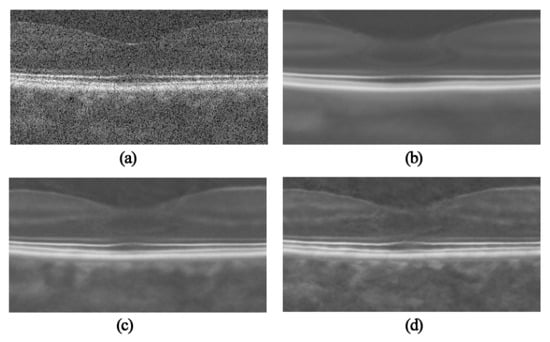
Figure 1.
Comparison of DIP denoising OCT image: (a) input noisy image, (b) constructed image with DIP speckle reduction after 500 iterations, (c) constructed image with DIP speckle reduction after 1000 iterations, (d) constructed image with DIP speckle reduction after 1500 iterations.
2.2. Non-Local Deep Image Prior Model
The convolutional neural networks (CNNs) have the intrinsic ability to solve inverse problems such as denoising without any pre-training. The main reason is that compared with the noise, the convolution layer is better able to recover the signal which has more self-similarity. However, for OCT despeckling, the DIP model has difficulty finding a good balance between maintaining details and suppressing speckle noise. One reason is that the L2 loss in Equation (4) does not distinguish between the differences originating from signal and noise.
The differences between the constructed image and the input image can be defined as:
As shown in Figure 2c, in the difference image, the signal shows stronger self-similarity than the noise. A sorted non-local statics is proposed in this section to measure the signal autocorrelation. Minimizing the signal autocorrelation of the difference image can make the network parameters converge more quickly with the OCT signals.
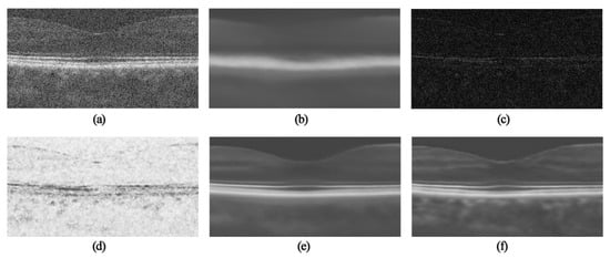
Figure 2.
NLM-DIP denoising OCT image: (a) input noisy image , (b) constructed image after 200 iterations, (c) absolute value of difference image between (a) and (b), (d) the uncorrelation of difference image, (e) constructed image with NLM-DIP speckle reduction after 450 iterations, (f) constructed image with NLM-DIP speckle reduction after 900 iterations.
We apply block matching to measure the non-local self-similarity in the difference image by calculating the correlation between the reference patch and each patch in the neighborhood . In this paper, the autocorrelation coefficient is applied as the metric:
where is the reference patch in difference image centered at , is the covariance of and , and and denote the standard deviation of and , respectively.
Note that the edge details in the difference image are not correlated with all their non-local neighborhood. To solve this problem, a sorted non-local statistic is proposed by sorting and selecting the mth largest autocorrelation coefficient. Based on the non-local statistic, the uncorrelation of difference image is obtained as follows:
where is the mth largest one among . It can be seen in Figure 2d, the statistic provides a measure of how independent a patch is to its most similar non-local neighbors in the difference image. The signal uncorrelation of the differences is obtained as follows:
The optimization loss function is therefore:
where the maximizes the signal uncorrelation or minimizes the signal autocorrelation in the difference image. The weight is used to balance two terms in the loss function.
Therefore, the parameters of the neural network can be trained by:
2.3. Network Structure and the NLM-DIP Algorithm
It can be seen from Figure 3 that the network structure employed in this work is based on the same U-Net type [] 5-layer “hourglass” architecture with skip-connections as DIP. The purpose of using an hourglass network is to repeatedly obtain information contained in images of different scales. The architecture consists of an encoding path (upper side) and a decoding path (lower side). Each scale of the encoding path consists of two 5 × 5 convolution layers, the first convolution layer with stride 2 for down-sampling. Each convolution layer is followed by a batch normalization (BN) and a leaky rectified linear unit (LReLU). Each scale of the decoding path consists of a 5 × 5 convolution layer, a 1 × 1 convolution layer and an up-sampling layer respectively, each convolution layer followed by the BN and the LReLU. As shown in Figure 3, the numbers of convolution kernels in the 5-layer network are 16, 32, 64, 128, and 128, respectively. The parameters of the neural network can be trained by the proposed reconstruction loss in Equation (11), as shown in Figure 3.
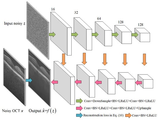
Figure 3.
The network structure used in this work.
The proposed NLM-DIP algorithm is summarized as follows:
| Algorithm NLM-DIP |
| Input: Maximum iteration number MaxIt, network initialization , noisy image and the network input (random noise). For to MaxIt do Calculate the signal uncorrelation of the differences using (9). Calculate the reconstruction loss using (10). Train the network using (11). End For Return . |
In each iteration, the input are perturbed with an additive normal noise which is used as a noise-based regularization. The proposed sorted non-local static selects most correlated patches () in the neighborhood . The in Equation (10) is used to balance the L1 loss and the proposed signal autocorrelation loss in the reconstruction function. In this paper, is set to 0.85 according to the experimental results. We set a learning rate of 0.001 and 900 iterations for the network training. Currently the code of the proposed NLM-DIP is not optimized and the network training was done in GPU (NVIDIA GTX1060). The neural network was implemented using PyTorch. Because the NLM-DIP needs to calculate and sort the non-local correlation coefficients in each iteration, it takes 0.40 s per iteration for a 900 × 450 OCT image, while the DIP takes 0.18 s per iteration.
3. Experimental Results
In this section, the proposed NLM-DIP is compared with TNode [], SBSDI [], PNLM [], and DIP [] on two types of retinal SDOCT image datasets []. The synthetic image dataset contains 18 spectral domain OCT (SDOCT) noise images generated from high resolution images that were then subsampled; each image was obtained by an 840 nm wavelength SDOCT imaging system from Bioptigen with an axial resolution of ~4.5 μm per pixel in the tissue. The real image dataset contains 39 SDOCT noise images acquired at a natively low sample rate.
3.1. OCT Despeckling Results
In order to facilitate the subjective comparison of the denoising effect, two images were randomly selected from the synthetic and the real image datasets, respectively. The experimental results are shown in Figure 4 and Figure 5. Figure 4a and Figure 5a are the original noisy OCT images. Figure 4b and Figure 5b are the TNode results which contain some noise. Figure 4c and Figure 5c show the SBSDI results. It can be seen that SBSDI allowed the recovery of most of the image information while containing some speckle noise. On the contrary, the PNLM results shown in Figure 4d and Figure 5d removed most speckle noise while losing some details. By contrast, the results of DIP and NLM-DIP are more natural-looking. Compared with DIP, NLM-DIP generally output smoother surfaces in homogeneous regions and maintained layer texture and boundary clarity without introducing artifacts.
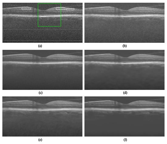
Figure 4.
Comparison of denoising OCT-15 image in the synthetic dataset: (a) original noisy image (900 × 450), (b) image after TNode speckle reduction, (c) image after SBSDI speckle reduction, (d) image after PNLM speckle reduction, (e) image after DIP speckle reduction, (f) image after NLM-DIP speckle reduction.
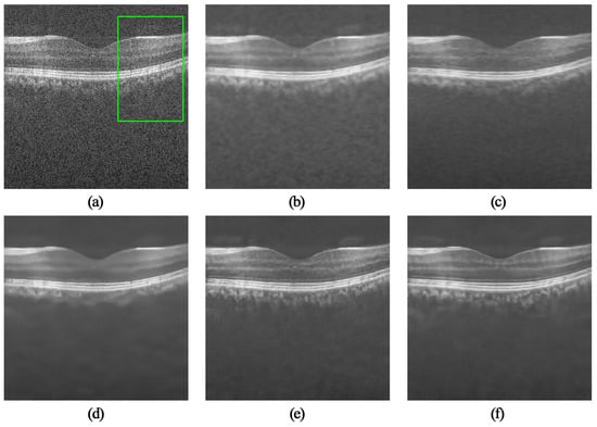
Figure 5.
Comparison of denoising OCT-26 image in the real dataset: (a) original noisy image (450 × 450), (b) image after TNode speckle reduction, (c) image after SBSDI speckle reduction, (d) image after PNLM speckle reduction, (e) image after DIP speckle reduction, (f) image after NLM-DIP speckle reduction.
In addition, some interesting areas in the field in the OCT image have been selected in Figure 4 and Figure 5 which are marked with green boxes, and the partial area is enlarged. The results are shown in Figure 6 and Figure 7. The TNode results show that the images containing noise and some local details were not clear. As can be seen from Figure 6c and Figure 7c, the SBSDI algorithm blurred the local layer structure of the image, and the denoised result still contained a slight noise. The PNLM algorithm performed well in low-intensity regions, but the layer structure of the denoised result was unclear. The results suggest the DIP algorithm can be used for OCT denoising, but the layer structure of the image was ambiguous. The NLM-DIP algorithm efficiently removed the speckle noise. In addition, it maintained the details and the layer structure of the image, which was beneficial to further layer segmentation or clinical diagnosis and analysis.
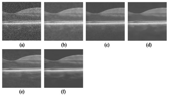
Figure 6.
Comparison of local layered structures of the green box in Figure 3. (a) Noisy image (256 × 256), results by (b) TNode, (c) SBSDI, (d) PNLM, (e) DIP, (f) NLM-DIP.
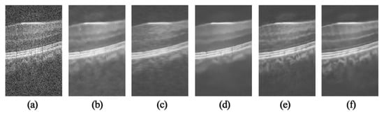
Figure 7.
Comparison of local layered structures of the green box in Figure 5. (a) Noisy image (256 × 160), results by (b) TNode, (c) SBSDI, (d) PNLM, (e) DIP, (f) NLM-DIP.
3.2. Image Quality Metrics
Considering that the experimental images in this chapter have been processed and compared with the clinical images of medical experiments, there is a lack of original images, and it is inconvenient to perform signal-to-noise ratio measurements. In order to make objective quantitative comparisons of various denoising methods, this section uses the average contrast to noise ratio (CNR) and the average equivalent number of looks (ENL) as evaluation measures. CNR measures the contrast level between the selected regions from the object in an image and the background region in the image. It can be calculated as:
where and are the mean and standard deviation of the th interest foreground region (e.g., the areas in solid rectangles inFigure 4a, and are the mean and standard deviation of the pixels in the background region (e.g., the dashed rectangle area in Figure 4a). ENL measures smoothness in areas that should have a homogeneous appearance but are corrupted by speckle:
To quantitatively compare different despeckling algorithms, we averaged the CNR and ENL images in the two datasets. It can be seen from Table 1 and Table 2 that the NLM-DIP algorithm provided the best despeckling performance in terms of CNR and ENL, compared with the other algorithm.

Table 1.
Metrics comparison of different despeckling algorithms on the synthetic dataset.
Table 2.
Metrics comparison of different despeckling algorithms on the real dataset.
4. Conclusions
Current advancements in neural networks show their great applicability for unsupervised signal preprocessing. In this paper, a non-local deep image prior network was proposed for OCT image restoration. By adding a sorted non-local statics as regularization loss in the DIP learning, more low-level image statistics were captured by CNN networks in the process of OCT image restoration. The experimental results show that the proposed NLM-DIP allowed the recovery of most of the OCT signal while getting rid of the speckle noise.
Author Contributions
Conceptualization, H.Y. and W.F.; software, W.F.; H.Y. and T.C.; writing—original draft preparation, W.F.; H.Y. and S.J.; supervision, H.Y. All authors have read and agree to the published version of the manuscript.
Funding
This work was supported in part by the Natural Science Foundation of China under grants 61971221.
Conflicts of Interest
The authors declare no conflict of interest.
References
- Choma, M.; Sarunic, M.; Yang, C.; Izatt, J. Sensitivity advantage of swept source and Fourier domain optical coherence tomography. Opt. Express 2003, 18, 2183–2189. [Google Scholar] [CrossRef]
- Farsiu, S.; Chiu, S.; O’Connell, J.; Folgar, F.; Yuan, E.; Izatt, A.J.; Toth, C. Quantitative classification of eyes with and without intermediate age-related macular degeneration using optical coherence tomography. Ophthalmology 2014, 121, 162–172. [Google Scholar] [CrossRef]
- Karamata, B.; Hassler, K.; Laubscher, M.; Lasser, T. Speckle statistics in optical coherence tomography. J. Opt. Soc. Am. A 2005, 22, 593–596. [Google Scholar] [CrossRef]
- Mayer, M.A.; Borsdorf, A.; Wagner, M.; Hornegger, J.; Mardin, C.Y.; Tornow, P.R. Wavelet denoising of multiframe optical coherence tomography data. Biomed. Opt. Express 2012, 3, 572–589. [Google Scholar] [CrossRef]
- Zaki, F.; Wang, Y.; Su, H.; Yuan, X.; Liu, X. Noise adaptive wavelet thresholding for speckle noise removal in optical coherence tomography. Biomed. Opt. Express 2017, 8, 2720–2731. [Google Scholar] [CrossRef] [PubMed]
- Jian, Z.; Yu, Z.; Yu, L.; Rao, B.; Chen, Z.; Tromberg, B.J. Speckle attenuation in optical coherence tomography by curvelet shrinkage. Opt. Lett. 2009, 34, 1516–1520. [Google Scholar] [CrossRef] [PubMed]
- Xu, J.; Ou, H.; Lam, E.Y.; Chui, P.C.; Wong, K.Y. Speckle reduction of retinal optical coherence tomography based on contourlet shrinkage. Opt. Lett. 2013, 38, 2900–2903. [Google Scholar] [CrossRef] [PubMed]
- Buades, A.; Coll, B.; Morel, J.M. A non-local algorithm for image denoising. In Proceedings of the IEEE Computer Society Conference on Computer Vision and Pattern Recognition, CVPR, San Diego, CA, USA, 20–25 June 2005; Volume 2, pp. 60–65. [Google Scholar]
- Aum, J.; Kim, J.; Jeong, J. Effective speckle noise suppression in optical coherence tomography images using nonlocal means denoising filter with double Gaussian anisotropic kernels. Appl. Opt. 2015, 54, D43–D50. [Google Scholar] [CrossRef]
- Yu, H.; Gao, J.; Li, A. Probability-based non-local means filter for speckle noise suppression in optical coherence tomography images. Opt. Lett. 2016, 41, 994–998. [Google Scholar] [CrossRef] [PubMed]
- Huang, S.; Chen, T.; Xu, M.; Qiu, Y.; Lei, Z. BM3D-based total variation algorithm for speckle removal with structure-preserving in OCT images. Appl. Opt. 2019, 58, 6233–6243. [Google Scholar] [CrossRef] [PubMed]
- Carlos, C.V.; René, R.; Bouma, B.E.; Néstor, U.P. Volumetric non-local-means based speckle reduction for optical coherence tomography. Biomed. Opt. Express 2018, 9, 3354–3372. [Google Scholar]
- Qi, G.; Zhang, Q.; Zeng, F.; Wan, J.; Zhu, Z. Multi-focus image fusion via morphological similarity-based dictionary construction and sparse representation. CAAI Trans. Intell. Technol. 2018, 3, 83–94. [Google Scholar] [CrossRef]
- Fang, L.; Li, S.; Nie, Q.; Izatt, J.A.; Toth, C.A.; Farsiu, S. Sparsity based denoising of spectral domain optical coherence tomography images. Biomed. Opt. Express 2012, 3, 927–942. [Google Scholar] [CrossRef] [PubMed]
- Fang, L.; Li, S.; McNabb, R.P.; Nie, Q.; Kuo, A.N.; Toth, C.A.; Izatt, J.A.; Farsiu, S. Fast acquisition and reconstruction of optical coherence tomography images via sparse representation. IEEE Trans. Med. Imaging Process. 2013, 32, 2034–2049. [Google Scholar] [CrossRef] [PubMed]
- Le, N.Q.K.; Ho, Q.T.; Ou, Y.Y. Incorporating deep learning with convolutional neural networks and position specific scoring matrices for identifying electron transport proteins. J. Comput. Chem. 2017, 38, 2000–2006. [Google Scholar] [CrossRef] [PubMed]
- Le, N.Q.K. Fertility-GRU: Identifying Fertility-Related Proteins by Incorporating Deep-Gated Recurrent Units and Original Position-Specific Scoring Matrix Profiles. J. Proteome Res. 2019, 18, 3503–3511. [Google Scholar] [CrossRef]
- Le, N.Q.K.; Yapp, E.K.Y.; Yeh, H.Y. ET-GRU: Using multi-layer gated recurrent units to identify electron transport proteins. BMC Bioinform. 2019, 20, 377. [Google Scholar] [CrossRef]
- Halupka, K.J.; Antony, B.J.; Lee, M.H.; Lucy, K.A.; Rai, R.S.; Ishikawa, H.; Wollstein, G.; Schuman, J.S.; Garnavi, R. Retinal optical coherence tomography image enhancement via deep learning. Biomed. Opt. Express 2018, 9, 6205–6221. [Google Scholar] [CrossRef]
- Qiu, B.; Huang, Z.; Liu, X.; Meng, X.; You, Y.; Liu, G.; Yang, K.; Maier, A.; Ren, Q.; Lu, Y. Noise reduction in optical coherence tomography images using a deep neural network with perceptually-sensitive loss function. Biomed. Opt. Express 2020, 11, 817–830. [Google Scholar] [CrossRef]
- Zhang, K.; Zuo, W.; Chen, Y.; Meng, D.; Zhang, L. Beyond a Gaussian Denoiser: Residual learning of deep CNN for image denoising. IEEE Trans. Image Process. 2017, 26, 3142–3155. [Google Scholar] [CrossRef]
- Priyanka, S.; Wang, Y.K. Fully symmetric convolutional network for effective image denoising. Appl. Sci. 2019, 9, 778. [Google Scholar] [CrossRef]
- Dong, W.; Wang, P.; Yin, W.; Shi, G. Denoising Prior Driven Deep Neural Network for Image Restoration. IEEE Trans. Pattern Anal. Mach. Intell. 2018, 41, 2305–2318. [Google Scholar] [CrossRef] [PubMed]
- Ulyanov, D.; Vedaldi, A.; Lempitsky, V. Deep Image Piror. In Proceedings of the IEEE Computer Society Conference on Computer Vision and Pattern Recognition, CVPR, Salt Lake City, UT, USA, 18–22 June 2018; pp. 9446–9454. [Google Scholar]
- Çiçek, Ö.; Abdulkadir, A.; Lienkamp, S.S.; Brox, T.; Ronneberger, O. 3D U-Net: Learning dense volumetric segmentation from sparse annotation. In Lecture Notes in Computer Science, Proceedings of International Conference Medical Image Computing and Computer-Assisted Intervention, MICCAI, Athens, Greece, 17–21 October 2016; Springer: Cham, Switzerland, 2016; pp. 424–432. [Google Scholar]
© 2020 by the authors. Licensee MDPI, Basel, Switzerland. This article is an open access article distributed under the terms and conditions of the Creative Commons Attribution (CC BY) license (http://creativecommons.org/licenses/by/4.0/).