Abstract
Optimal tuning of particle accelerators is a challenging task. Many different approaches have been proposed in the past to solve two main problems—attainment of an optimal working point and performance recovery after machine drifts. The most classical model-free techniques (e.g., Gradient Ascent or Extremum Seeking algorithms) have some intrinsic limitations. To overcome those limitations, Machine Learning tools, in particular Reinforcement Learning (RL), are attracting more and more attention in the particle accelerator community. We investigate the feasibility of RL model-free approaches to align the seed laser, as well as other service lasers, at FERMI, the free-electron laser facility at Elettra Sincrotrone Trieste. We apply two different techniques—the first, based on the episodic Q-learning with linear function approximation, for performance optimization; the second, based on the continuous Natural Policy Gradient REINFORCE algorithm, for performance recovery. Despite the simplicity of these approaches, we report satisfactory preliminary results, that represent the first step toward a new fully automatic procedure for the alignment of the seed laser to the electron beam. Such an alignment is, at present, performed manually.
1. Introduction
In a seeded Free-Electron Laser (FEL) [1,2,3,4], the generation of the FEL process is based on the overlap of a ∼1 -long bunch of relativistic electrons with a ∼100 pulse of photons of an optical laser, which takes place inside a static magnetic field generated by specific devices called undulators. Both the longitudinal (temporal) and transverse superposition are crucial for attaining the FEL process and therefore they must be controlled precisely. The former is adjusted by means of a single mechanical delay line placed in the laser path, while the latter has several degrees of freedom as it involves the trajectories of the electron and laser beams inside the undulators. A shot-to-shot feedback system based on position sensors [5] has been implemented, at the Free Electron laser Radiation for Multidisciplinary Investigations (FERMI), to keep the electron trajectory stable, while the trajectory of the laser has to be continuously readjusted being subject to thermal drifts or restored whenever the laser transverse profile changes because the FEL operators modify the laser wavelength.
During standard operations, the horizontal and vertical transverse position and angle (pointing) of the laser beam inside the undulators is kept optimal by an automatic process exploiting the correlation of the FEL intensity with the natural noise of the trajectory [6]. Whenever the natural noise is not sufficient to determine in which direction to move the pointing of the laser, artificial noise can be injected. This method improves the convergence of the optimization, but the injected noise can affect the quality of the FEL radiation. This kind of model-free optimization techniques (ex. Gradient Ascent and Extremum Seeking [7,8]) are widely used in FEL facilities, but have some intrinsic disadvantages:
- the need to evaluate the gradient of the objective function, which can be difficult to estimate when the starting point is far from the optimum;
- the difficulty to determine the hyper-parameters, whose appropriate values depend on the environment and the noise of the system;
- the lack of “memory” to exploit the past experience.
Modern algorithms like Reinforcement Learning (RL), which belong to the category of Machine Learning (ML), are able to automatically discover the hidden relationship between input variables and objective function without human supervision. Although they usually require large amounts of data sets and long leaning time, they are becoming popular in the particle accelerator community thanks to their capability to work with no knowledge of the system.
In order to optimize the FEL’s performance, different approaches have been adopted in recent years [9]. In 2011, a multi-physics simulation tool kit designed for the study of FELs and synchrotron light sources called OCELOT [10] was developed at the European XFEL GmbH. In addition to some common generic optimization algorithms (Extremum Seeking, Nelder-Mead) the framework implements Bayesian optimization based on Gaussian process. This tool is routinely employed in tuning of quadrupole currents at the Stanford Linear Accelerator Center (SLAC) [11,12] and optimization of the self-amplification power of the spontaneous emission (SASE) for the Free electron LASer in Hamburg (FLASH) at the Deutsches Elektronen-SYnchrotron (DESY) [13]. A different approach is described in Reference [14], where the authors advocate the use of artificial neural networks to model and control particle accelerators; they also mention applications based on the combination of neural networks and RL methods. Finally, recent works [15,16,17,18] have presented RL methods used in the context of particle accelerators. In References [15] and [16], performed through simulations, the FEL model and the policy are defined by neural networks. In Reference [17] the authors present an application of RL on a real system. The study concerns a beam alignment problem faced with a deep Q-learning approach in which the state is defined as the beam position.
The present paper is actually an extended version of Reference [18], in which Q-Learning with linear function approximation was used to perform the alignment of the seed laser. Here, we use an additional well-known RL technique, namely the Natural Policy Gradient (NPG) version of the REINFORCE algorithm [19] (NPG REINFORCE). It allows us to operate on a continuous space of actions that adapts itself to an underlying model changing over time. In fact, while in Reference [18] the goal was to control the overlap of electrons and laser beams starting from random initial conditions, in this paper we also deal with the problem of machine drifts. For the latter, we use NPG REINFORCE. The target of our study is the FERMI FEL (Section 3), one of the few 4th-generation light source facilities available in the world. Due to its intensive use, its availability for testing the algorithms is very limited. Therefore, some preliminary experiments have been conducted on a different system, namely the Electro-Optical Sampling station (EOS) (Section 2). Despite the differences between the two systems, they lead to similar problem formulations of RL. Both techniques have finally been implemented on the FERMI FEL.
The rest of the article is organized as follows—Section 2 and Section 3 introduce the physical systems of EOS and FEL. Basic information on our implementation of the RL algorithms is provided in Section 4, while the experimental configuration and the achieved results are described in Section 5. Finally, conclusions are drawn in Section 6.
2. EOS Alignment System
The considered optical system is part of the EOS station, located upstream of the second line of the free-electron laser. The EOS is a non destructive diagnostics device designed to perform on-line single-shot longitudinal profile and arrival time measurements of the electron bunches using an UV laser [20,21,22]. Since the aim of the present work is to control a part of the laser trajectory, we will not explain in details the EOS process, but rather we will focus on the parts of the device relevant for our purpose.
The device, simplified in Figure 1, is a standard optical alignment system composed of two planar tip-tilt mirrors [23] (TTs), each driven by two couples of motors. Coarse positioning is obtained via two coarse-motors, while two piezo-motors are employed for fine-tuning. In the optimization process, only the piezo-motors are considered.Two charge-coupled devices (CCDs) detect the position of the laser beam in two different places along the path (the CCDs do not intercept the laser beam thanks to the use of semi-reflecting mirrors).
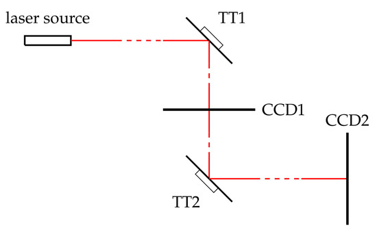
Figure 1.
Simple scheme of the Electro-Optical Sampling station (EOS) laser alignment set up. TT1 and TT2 are the tip-tilt mirrors (TTs) while CCD1 and CCD2 are the charge-coupled devices (CCDs).
The ultimate goal is to steer and keep the laser spot inside a pre-defined region of interest (ROI) of each CCD. To achieve this result, a proper voltage has to be applied to each piezo-motor. The product of the two light intensities detected by the CCDs in the ROIs can be used as an evaluation criterion for the correct positioning of the laser beam. In particular, it can be interpreted as an AND logic operator, that is “true” when the laser is inside both of the ROIs.
3. FEL Alignment System
In a seeded FEL, an initial seed signal, provided by a conventional high peak power pulsed laser, is temporally synchronized to overlap the electron bunches inside a first undulator section called modulator. In the transverse alignment process two Yttrium Aluminum Garnet (YAG) screens equipped with CCDs are properly inserted and extracted, in order to measure the electron beam transverse position before and after the modulator [24]. After the electron beam inhibition, using the same YAG screens, the seed laser position is measured and the correct positions of two tip-tilt mirrors are manually found by moving the coarse-motors in order to overlap the electron beam. The above destructive (a screen has to be inserted) procedure is repeated several times and, at the end, the screens are removed to switch on the FEL. The simplified scheme of the alignment set up is shown in Figure 2. After the above described coarse tuning, a further optimization is carried out by moving the tip-tilt mirrors to maximize the FEL intensity measured by the monitor. The working principle of this monitor is the atomic photo-ionization of a rare gas at low particle density in the range of ( mbar). The FEL photon beam, traveling through a rare gas-filled chamber, generates ions and electrons, which are extracted and collected separately. From the resulting currents it is possible to derive the absolute number of photons per pulse, shot by shot.
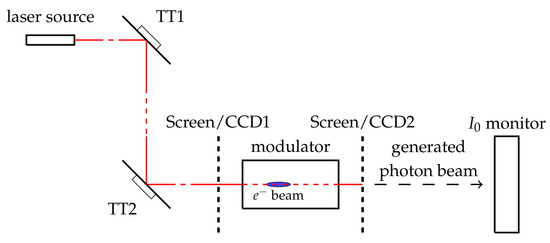
Figure 2.
Simple scheme of the FERMI FEL seed laser alignment set up. TT1 and TT2 are the tip-tilt mirrors, Screen/CCD1 and Screen/CCD2 are the two removable YAG screens with CCDs and monitor is the employed intensity sensor.
4. Reinforcement Learning
In RL, basically, data collected through experience are employed to select future inputs of a dynamical system [25,26]. An environment is a discrete dynamical system whose model can be defined by:
in which and respectively are the environment state and the external control input (the action) at the k-th instant; while f is the state-transition function. A controller, or agent, learns a suitable state-action map, also known as policy (), by interacting with the environment through a trial and error process. For each chosen action , in state , the environment provides a reward . The aim of the learning process is to find an optimal policy with respect to the maximization of an objective function J, which is a design choice.
4.1. Q-Learning
Among the different approaches to the RL problem, the approximate dynamic programming aims at solving the problem
in which is the discount factor, by iteratively estimating an action-value function (or Q-function) from data. Here, J takes the form of an expected discounted cumulative reward. Assuming that there exists a stationary (stationarity is the consequence of the infinite time horizon, i.e., , and implies that the optimal action for a given state x at time k depends only on x and not on k). Optimal policy, the Q-function is defined as the optimum value of the expected discounted reward when action u is selected being in state x. Therefore, given the action-value function , the optimal policy is
In other words, estimating the Q-function amounts to solving the learning problem. An attractive and well-known method for estimating the Q-function is the Q-learning algorithm [27].
In the present work, we employ the Q-learning in an episodic framework (meaning that the learning is split into episodes that end when some terminal conditions are met). The choice of the Q-learning among other RL approaches is due to its simplicity and the fact that the problem admits a non-sparse reward which is beneficial for speeding up the learning [28]. During learning, the exploration of the state-action space can be achieved by employing a so-called -greedy policy:
in which defines the probability of a random choice (exploration). The Q-learning update rule is:
where is the learning rate and is the temporal difference error, the difference between the discounted optimal Q in the state and the value (see Algorithm 1 for more details). Defining the state set as (where n is the dimension of the state vector), since the actions are finite (), the action-value function can be represented as a collection of maps from to . In order to work with a continuous state space, we employ a linear function approximation version of the Q-learning algorithm. More precisely, we parametrize each as , where is a vector of features and a weight vector associated to the j-th input . Thus, the whole is specified by the vector of parameters , and the corresponding policy will be identified by . In particular, we employ Gaussian Radial Basis Functions (RBFs) as features; given a set of centers , we set in which is:
where determines the decay rate of RBF. The pseudo code of the Q-learning with linear function approximation is reported in Algorithm 1.
| Algorithm 1 Q-learning algorithm with linear function approximation [29] |
Initialize and set , For each episode:
|
4.2. Policy Gradient REINFORCE
An alternative approach consists of directly learning a policy, without relying on value functions. In this regard, given a policy parametrized by a vector , Policy Gradient (PG) methods [26] aim at finding an optimal which ensures to
in which is a state-input trajectory obtained by following a particular , and is the corresponding cumulative reward. The trajectory can be thought of as a random variable that has a probability distribution . We employ the REINFORCE algorithm [19] which aims at finding the optimal for , solution of the optimization problem (5), by updating along gradient of the objective function. More precisely, a stochastic gradient ascent is performed:
where is the learning rate. Since , where is the transition probability from to when the action is applied, the update rule (6) becomes:
Such an update is performed every time a path is collected. In order to reduce the variance of the gradient estimates, typical of the PG approaches [30], we employ a NPG version [31] of the REINFORCE algorithm, in which a linear transformation of the gradient is adopted by using the inverse Fisher information matrix . The pseudo code of the REINFORCE is reported in Algorithm 2.
| Algorithm 2 REINFORCE |
Set and set While :
|
5. Implementation and Results
In the following we apply the two different RL techniques described above, to address the two problems:
- the attainment of an optimal working point, starting from random initial conditions;
- the recovery of the optimal working point when some drifts, or working conditions changes, occur.
The former employs the Q-Learning, the latter through the NPG REINFORCE algorithm. The reason is their simplicity. In particular, for the problem of target recovery, the policy gradient algorithm REINFORCE has been chosen to employ a continuous action space, which allows fine adjustments to compensate small drifts. Both algorithms have been tested on the EOS system before being deployed on the FEL system. In the present section we describe the experimental protocols, and we report the results, that will be discussed in Section 5.3.
5.1. Optimal Working Point Attainment Problem
The problem of defining a policy, able to lead the plant to an optimal working point starting from random initial conditions, requires to split the experiments in two phases: (i) a training, which allows the controller to learn a proper policy, and (ii) a test, to validate the ability of the learned policy to properly behave, possibly in conditions not experienced during training.
In both the optical systems—the EOS and the FEL—the state x is a 4 dimensional vector that provides the current voltage values applied to each piezo-motor (two values for the first mirror and two values for the second mirror). We neglect the dynamics of the piezo-motors, being their transients much shorter than the time between shots. The input u is also a 4 dimensional vector; denoting the component index as a superscript, the update rule is:
that is, the input is the incremental variation of the state itself. The action space is discrete, thus the module of each i-th component of u is set equal to a fixed value. Moreover, the state x can only assume values that satisfy the physical constraints of the piezo-motors [23]:
hence we allow, for each state x of both systems, only those inputs u for which the component-wise inequality (8) is not violated. In the following, when referring to the intensity of the EOS, we will actually refer to the product of the two intensities detected in the ROIs when the laser hits both ROIs; by FEL intensity, we will mean the intensity measured by the monitor. Finally, for both systems, we will denote the target intensity (computed as explained below) as .
5.1.1. EOS
The training of the EOS alignment system consists of 300 episodes. The number of episodes has been chosen after preliminary experiments on a EOS device simulator. However, based on the results obtained on the real device, the number of episodes can be actually reduced (see Figure 3). At the beginning of the training, the ROIs are selected, and therefore also the target value . They remain the same for all the training episodes. At each time step k, the input provided by the agent is applied, and the new intensity is compared with the target (). The episode ends in two cases:
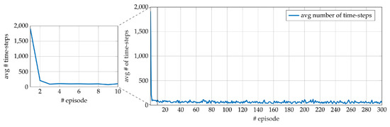
Figure 3.
Average number of time-steps for each episode during the 10 runs in training performed on the EOS system. The average number of time-steps required in the first 10 episodes is highlighted in the enlarged portion.
- when the detected intensity in the new state is greater than or equal to a certain percentage of the target ();
- when the maximum number of allowed time steps is reached.
When the first statement occurs, the goal is achieved. During the training procedure the values of (exploration) of (2) and (learning rate) of (3), decay according to the following rules [32,33]:
where the value is set empirically. In addition, the reward is shaped according to [28]:
where is taken equal to 1 if the target is reached, 0 otherwise; the values of and are set empirically. The specific design of (10) allows to reward the agent in correspondence of state-action pairs that lead to a sufficiently increased detected intensity () and to penalize it otherwise (). At the end of each episode a new one begins from a new initial state, randomly selected, until the maximum number of episodes is reached. Then, a test (with random initial states) is carried out for the same target conditions of the training but with a fixed as in Reference [34] and . We repeat the training and test 10 times (i.e., we perform 10 different runs) and report in the following the results in terms of average duration of each episode. The parameter values employed during experiments are reported in Table 1; they result from offline experiments on a simulator of the EOS system.

Table 1.
Parameters used in EOS Q-learning.
The average number of time-steps per episode for the whole training phase is reported in Figure 3. The steep decrease of the average number of time steps shows that a few episodes are sufficient to get a performance close to the one obtained after a whole training phase. Indeed, thanks to the reward shaping (10), the Q-function is updated at each step of each episode instead of just at the end of the episode (see Section 5.3 for further details). The average number of time-steps per episode during the test phase is visible in Figure 4 and is consistent with the training results.
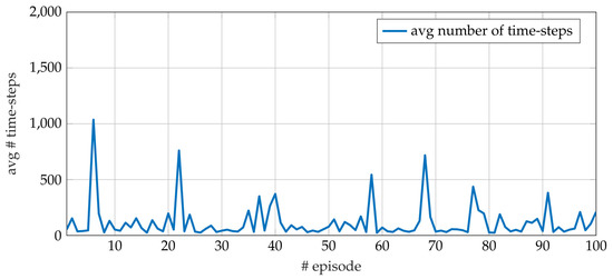
Figure 4.
Average number of time-steps for each episode during the 10 runs in the test performed on the EOS system.
5.1.2. FEL
The experiment carried out on the FEL system consists of a training of 300 episodes and a test of 50 episodes. The chosen target value is kept constant throughout the whole training and test. At the beginning of each episode, a random initialization is applied. Each episode ends when the same conditions defined in Section 5.1.1 occur. The and the values decay according to (9) and the reward is shaped in the same way of the EOS case. The parameter values are reported in Table 2.
Table 2.
Parameters used in FERMI free electron laser (FEL) Q-learning.
The results are reported in Figure 5 and Figure 6, for training and test respectively. It can be observed that the overall behaviors, in training and test, resemble those in Figure 3 and Figure 4.
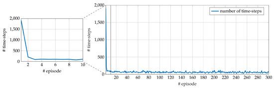
Figure 5.
Number of time-steps for each episode during a single run of training performed on the FERMI FEL system. The number of time-steps required in the first 10 episodes is highlighted in the enlarged portion.
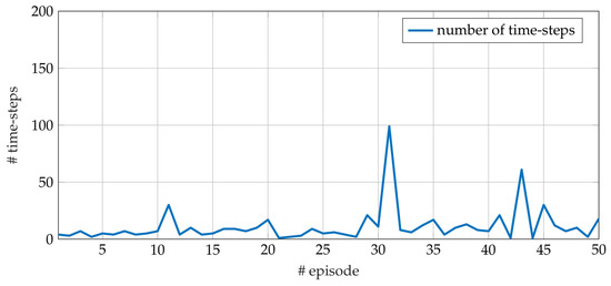
Figure 6.
Number of time-steps for each episode during a single run of test performed on the FERMI FEL system.
5.2. Recovery of Optimal Working Point
In particle accelerator facilities, the working conditions are constantly subject to fluctuations. Indeed, thermal drifts or wavelength variations requested by users are common and result in a displacement of the optimal working point. Therefore, a controller must be able to quickly and properly adapt its policy to such drifts. For this purpose, we adopt the NPG REINFORCE algorithm (Section 4.2), which is able to work with a continuous action space and, thus, to allow for precise fine tuning. Here, we want to employ the learning as an adaptive mechanism, to face the machine drifts. Thus, in this case, a test phase would be meaningless, since adaptation occurs during learning only.
For both the optical systems, the EOS and the FEL, the state is a four-dimensional vector of the voltage values applied to each piezo-motor (two values for the first mirror and two values for the second mirror) and the action is composed of four references, one for each piezo-motor actuators, from which the new state depends.
The agent consists of four independent parametrized policies, one for each element of the action vector (), which are shaped according to the Von Mises distribution (such a distribution is a convenient choice when the state and action spaces are bounded, since it is null outside a bounded region):
where is a concentration measure, is the mean, is the modified Bessel function of the first kind [35] and is the i-th policy parameter vector, updated at each step of the procedure.
At each training step k, when the system is in state , the agent performs an action , according to the current policy, thus leading the system in a new state . Then, the intensity is detected and the reward is computed according to:
where is the target intensity. In the EOS system, in order to emulate drifts of the target condition, is initialized by averaging values collected at the beginning of the training procedure and then updated, each time that results greater than , according to:
In the FEL, however, we initialize the system in a manually found optimal setting (including both the state and the ), and impose some disturbances manually. The possibility to update the target intensity is still enabled though.
5.2.1. EOS
The NPG REINFORCE experiment performed on the EOS system consists of a single training phase, at the beginning of which the EOS system is randomly initialized, as well as the . The learning rate (7) is kept constant and equal to (empirical setting). Only when the detected intensity assumes a value greater than , is the latter updated according to (12) and the algorithm continues with the new target to be reached. The procedure is stopped when vectors lead each Von Mises distributions enough close to Dirac delta functions, after no target update has been performed for a predefined time. Figure 7 shows the detected intensity (blue line), its moving average (green line) and the target intensity (red dashed line) during the experiment. In Figure 8, the reward (blue line) is reported along with its moving average (green line) and the target (red dashed line). By comparing the two figures, it can be seen that once the target does not change, the reward approaches zero and the detected intensity variance shrinks, evidence that the optimal working point is close.
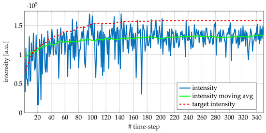
Figure 7.
Intensity during a single run of Natural Policy Gradient (NPG) REINFORCE on EOS. The blue line represents the detected intensity, while the green line is its moving average obtained with a fixed window size of 50 samples. The dashed red line represents the target intensity. Until time-step 200 the improvement of the intensity is appreciable; a further evidence is the update of the target intensity. In the remaining time-steps, the target intensity exhibits only small updates.
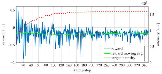
Figure 8.
Reward (blue), moving average of reward (green) with a fixed window size of 50 samples and target intensity (red, dashed) during a single run of NPG REINFORCE on EOS. The target intensity increases each time a reward greater than zero is observed.
5.2.2. FEL
Even in this case, the experiment consists of a single training phase, at the beginning of which, however, the system is set on an optimal working point, manually found by experts. During the experiment, some misalignment are forced by manually changing the coarse motors position. The learning rate of (7) is kept constant and equal to an empirically set value ().
Figure 9 and Figure 10 report the detected intensity and the reward, together with the target, during the execution of the NPG REINFORCE algorithm on the FEL. It can be seen that, contrary to the EOS experiment, the target intensity is not significantly updated. Indeed, in this case the system is initialized on an optimal working point. Two drift events took place, the first around time-step 120, and the second around time-step 210. Both plots, (detected intensity and reward), clearly show the capability to recover an optimal working point.
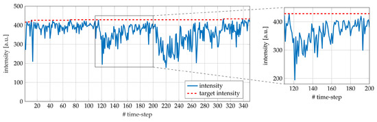
Figure 9.
Intensity during a single run of NPG REINFORCE on FEL. The blue line represents the detected intensity. The dashed red line represents the target intensity. The target intensity is almost constant during the whole run. Two perturbations have been manually introduced by moving the coarse motors. It is possible to appreciate the capability to recover FEL intensity in both events. The first perturbation and subsequent recovery are highlighted in the enlarged portion.
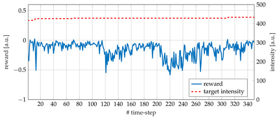
Figure 10.
Reward (blue) and target intensity (red, dashed) during a single run of NPG REINFORCE on FEL. The slight increases of target intensity correspond to positive rewards.
5.3. Discussion
The results obtained on EOS and FEL systems during experiments and presented above deserve some further comments that are provided here. The Q-learning algorithm has been applied to face the problem of finding an optimal working point, starting from a random initialization. The results are reported in Section 5.1. The enlarged portions reported in Figure 3 and Figure 5 show that a few episodes are sufficient to drastically reduce the number of steps required to reach the goal. In other words, the exploration carried out during the first episodes provides a valuable information for the estimation of the Q-function and, as a consequence, of an appropriate policy. We believe that the main reason is the effectiveness of the reward shaping (10), that allows for obtaining a reward at each time step, as opposite of a sparse reward occurring only at the end of the episodes. Such a shaping seems reasonable for the problem at hand, and is based on the assumption that the observed intensity change of two subsequent steps is significant for guiding the learning. On the other hand, during the test phase, we have observed that some unsuccessful trials occur. Although some further investigation is needed, it might be due to either (i) the occurrence of unexpected drifts of the target during the test or (ii) the discrete set of actions employed, consisting of fixed steps that can prevent reaching the goal, starting from random initial conditions.
The NPG REINFORCE algorithm has been applied for restoring the optimal working point in case of drifts. The results are reported in Section 5.2. In particular, Figure 9 and Figure 10 show the response to manual perturbations of the FEL operating conditions, set initially in an optimal working point. It is possible to observe how the algorithm quickly replies to disturbances of environment settings (marked by negative reward spikes), by learning a policy able to recover the optimal pointing of the laser.
6. Conclusions
Two tasks of particle accelerator optimal tuning have been addressed in this paper, namely (i) the attainment of the optimal working point and (ii) its recovery after a machine drift. Accordingly, two appropriate RL techniques have been employed: an the episodic Q-learning with linear function approximation, to reach the optimal working point starting from a random initialization, and a non-episodic NPG REINFORCE, to recover the performance after machine drifts or disturbances. Both approaches have been applied on the service laser alignment in the electro-optical sampling station before being successfully implemented on the FERMI free-electron laser at Elettra Sincrotrone, Trieste.
Based on the promising results, further investigation on free-electron laser optimization via automatic procedures will be carried out. Among some other approaches that could be investigated, we mention the normalized advantage functions [36], a continuous variant of the Q-learning, and the iterative linear quadratic regulator [37].
Author Contributions
Supervision, M.L. and F.A.P.; Conceptualization, N.B., G.F., F.H.O. and F.A.P.; Formal analysis, N.B., G.F., F.H.O., F.A.P. and E.S.; Investigation, validation and data curation, N.B., G.G. and F.H.O. Writing—Original draft, N.B. and E.S.; Writing—Review and editing, G.F., G.G., M.L. and F.A.P. All authors have read and agreed to the published version of the manuscript.
Funding
This research was partially funded by the Italian Ministry for Research in the framework of the 2017 Program for Research Projects of National Interest (PRIN), Grant no. 2017YKXYXJ.
Conflicts of Interest
The authors declare no conflict of interest.
Abbreviations
The following abbreviations are used in this manuscript:
| FEL | Free-Electron Laser |
| FERMI | Free Electron laser Radiation for Multidisciplinary Investigations |
| ML | Machine Learning |
| RL | Reinforcement Learning |
| SLAC | Stanford Linear Accelerator Center |
| DESY | Deutsches Elektronen-SYnchrotron |
| SASE | Self-Amplified Spontaneous Emission |
| FLASH | Free-electron LASer in Hamburg |
| NPG | Natural Policy Gradient |
| EOS | Electro-Optical Sampling |
| TT | Tip-Tilt |
| CCD | Charge-Coupled Device |
| ROI | Region Of Interest |
| YAG | Yttrium Aluminium Garnet |
| RBF | Radial Basis Function |
| PG | Policy Gradient |
References
- Yu, L.H. Generation of intense UV radiation by subharmonically seeded single-pass free-electron lasers. Phys. Rev. A 1991, 44, 5178. [Google Scholar] [CrossRef] [PubMed]
- Allaria, E.; Badano, L.; Bassanese, S.; Capotondi, F.; Castronovo, D.; Cinquegrana, P.; Danailov, M.; D’Auria, G.; Demidovich, A.; De Monte, R.; et al. The FERMI free-electron lasers. J. Synchrotron Radiat. 2015, 22, 485–491. [Google Scholar] [CrossRef] [PubMed]
- Allaria, E.; Appio, R.; Badano, L.; Barletta, W.; Bassanese, S.; Biedron, S.; Borga, A.; Busetto, E.; Castronovo, D.; Cinquegrana, P.; et al. Highly coherent and stable pulses from the FERMI seeded free-electron laser in the extreme ultraviolet. Nat. Photonics 2012, 6, 699. [Google Scholar] [CrossRef]
- Allaria, E.; Castronovo, D.; Cinquegrana, P.; Craievich, P.; Dal Forno, M.; Danailov, M.; D’Auria, G.; Demidovich, A.; De Ninno, G.; Di Mitri, S.; et al. Two-stage seeded soft-X-ray free-electron laser. Nat. Photonics 2013, 7, 913. [Google Scholar] [CrossRef]
- Gaio, G.; Lonza, M. Evolution of the FERMI beam based feedbacks. In Proceedings of the 14th International Conference on Accelerator & Large Experimental Physics Control Systems (ICALEPCS), San Francisco, CA, USA, 6–11 October 2013; pp. 1362–1365. [Google Scholar]
- Gaio, G.; Lonza, M.; Bruchon, N.; Saule, L. Advances in Automatic Performance Optimization at FERMI. In Proceedings of the 16th International Conference on Accelerator & Large Experimental Physics Control Systems (ICALEPCS), Barcelona, Spain, 8–13 October 2017. [Google Scholar]
- Ariyur, K.B.; Krstić, M. Real-Time Optimization by Extremum-Seeking Control; John Wiley & Sons: New York, NY, USA, 2003. [Google Scholar]
- Bruchon, N.; Fenu, G.; Gaio, G.; Lonza, M.; Pellegrino, F.A.; Saule, L. Free-electron laser spectrum evaluation and automatic optimization. Nucl. Instrum. Methods Phys. Res. Sect. A Accel. Spectrom. Detect. Assoc. Equip. 2017, 871, 20–29. [Google Scholar] [CrossRef][Green Version]
- Tomin, S.; Geloni, G.; Zagorodnov, I.; Egger, A.; Colocho, W.; Valentinov, A.; Fomin, Y.; Agapov, I.; Cope, T.; Ratner, D.; et al. Progress in Automatic Software-based Optimization of Accelerator Performance. In Proceedings of the 7th International Particle Accelerator Conference (IPAC), Busan, Korea, 8–13 May 2016. [Google Scholar]
- Agapov, I.; Geloni, G.; Tomin, S.; Zagorodnov, I. OCELOT: A software framework for synchrotron light source and FEL studies. Nucl. Instrum. Methods Phys. Res. Sect. A Accel. Spectrom. Detect. Assoc. Equip. 2014, 768, 151–156. [Google Scholar] [CrossRef]
- McIntire, M.; Cope, T.; Ratner, D.; Ermon, S. Bayesian optimization of FEL performance at LCLS. In Proceedings of the 7th International Particle Accelerator Conference (IPAC), Busan, Korea, 8–13 May 2016. [Google Scholar]
- McIntire, M.; Ratner, D.; Ermon, S. Sparse Gaussian Processes for Bayesian Optimization. In Proceedings of the Thirty-Second Conference on Uncertainty in Artificial Intelligence (UAI), Arlington, VA, USA, 25–29 June 2016. [Google Scholar]
- Agapov, I.; Geloni, G.; Zagorodnov, I. Statistical optimization of FEL performance. In Proceedings of the 6th International Particle Accelerator Conference (IPAC), Richmond, VA, USA, 3–8 May 2015. [Google Scholar]
- Edelen, A.; Biedron, S.; Chase, B.; Edstrom, D.; Milton, S.; Stabile, P. Neural networks for modeling and control of particle accelerators. IEEE Trans. Nucl. Sci. 2016, 63, 878–897. [Google Scholar] [CrossRef]
- Edelen, A.L.; Edelen, J.P.; RadiaSoft, L.; Biedron, S.G.; Milton, S.V.; van der Slot, P.J. Using Neural Network Control Policies For Rapid Switching Between Beam Parameters in a Free-Electron Laser. In Proceedings of the 31st Conference on Neural Information Processing Systems (NIPS), Long Beach, CA, USA, 8 December 2017. [Google Scholar]
- Edelen, A.L.; Milton, S.V.; Biedron, S.G.; Edelen, J.P.; van der Slot, P.J.M. Using A Neural Network Control Policy For Rapid Switching Between Beam Parameters in an FEL; Technical Report; Los Alamos National Lab (LANL): Los Alamos, NM, USA, 2017. [Google Scholar]
- Hirlaender, S.; Kain, V.; Schenk, M. New Paradigms for Tuning Accelerators: Automatic Performance Optimization and First Steps Towards Reinforcement Learning at the CERN Low Energy Ion Ring. In Proceedings of the 2nd ICFA Workshop on Machine Learning for Charged Particle Accelerators, PSI, Villigen, Switzerland, 26 February–1 March 2019; Available online: https://indico.cern.ch/event/784769/contributions/3265006/attachments/1807476/2950489/CO-technical-meeting-_Hirlaender.pdf (accessed on 31 March 2020).
- Bruchon, N.; Fenu, G.; Gaio, G.; Lonza, M.; Pellegrino, F.A.; Salvato, E. Toward the Application of Reinforcement Learning to the Intensity Control of a Seeded Free-Electron Laser. In Proceedings of the 23rd International Conference on Mechatronics Technology (ICMT), Salerno, Italy, 23–26 October 2019; Senatore, A., Dinh, T.Q., Eds.; IEEE: Piscataway, NJ, USA, 2019; pp. 1–6. [Google Scholar]
- Williams, R.J. Simple statistical gradient-following algorithms for connectionist reinforcement learning. Mach. Learn. 1992, 8, 229–256. [Google Scholar] [CrossRef]
- Veronese, M.; Allaria, E.; Cinquegrana, P.; Ferrari, E.; Rossi, F.; Sigalotti, P.; Spezzani, C. New Results Of Fermi Fel1 Eos Diagnostics With Full Optical Synchronization. In Proceedings of the 3rd International Beam Instrumentation Conference (IBIC), Monterey, CA, USA, 14–18 September 2014. [Google Scholar]
- Veronese, M.; Danailov, M.; Ferianis, M. The Electro-Optic Sampling Stations For FERMI@ Elettra, a Design Study. In Proceedings of the 13th Beam Instrumentation Workshop (BIW), Tahoe City, CA, USA, 4–8 May 2008. [Google Scholar]
- Veronese, M.; Abrami, A.; Allaria, E.; Bossi, M.; Danailov, M.; Ferianis, M.; Fröhlich, L.; Grulja, S.; Predonzani, M.; Rossi, F.; et al. First operation of the electro optical sampling diagnostics of the FERMI@ Elettra FEL. In Proceedings of the 1st International Beam Instrumentation Conference (IBIC), Tsukuba, Japan, 1–4 October 2012; Volume 12, p. 449. [Google Scholar]
- Cleva, S.; Pivetta, L.; Sigalotti, P. BeagleBone for embedded control system applications. In Proceedings of the 14th International Conference on Accelerator & Large Experimental Physics Control Systems (ICALEPCS), San Francisco, CA, USA, 6–11 October 2013. [Google Scholar]
- Gaio, G.; Lonza, M. Automatic FEL optimization at FERMI. In Proceedings of the 15th International Conference on Accelerator and Large Experimental Control Systems (ICALEPCS), Melbourne, Australia, 17–23 October 2015. [Google Scholar]
- Sutton, R.S.; Barto, A.G. Reinforcement Learning: An Introduction; MIT Press: Cambridge, MA, USA, 2018. [Google Scholar]
- Recht, B. A tour of reinforcement learning: The view from continuous control. Ann. Rev. Control Robot. Auton. Syst. 2018, 2, 253–279. [Google Scholar] [CrossRef]
- Watkins, C.J.; Dayan, P. Q-learning. Mach. Learn. 1992, 8, 279–292. [Google Scholar] [CrossRef]
- Ng, A.Y.; Harada, D.; Russell, S. Policy invariance under reward transformations: Theory and application to reward shaping. In Proceedings of the 16th International Conference on Machine Learning (ICML), Bled, Slovenia, 27–30 June 1999; Volume 99, pp. 278–287. [Google Scholar]
- Szepesvári, C. Algorithms for reinforcement learning. Synth. Lect. Artif. Intell. Mach. Learn. 2010, 4, 1–103. [Google Scholar] [CrossRef]
- Zhao, T.; Hachiya, H.; Niu, G.; Sugiyama, M. Analysis and improvement of policy gradient estimation. In Proceedings of the 25th Conference on Neural Information Processing Systems (NIPS), Granada, Spain, 12–17 December 2011. [Google Scholar]
- Kakade, S.M. A natural policy gradient. In Proceedings of the 15th Conference on Neural Information Processing Systems (NIPS), Vancouver, BC, Canada, 3–8 December 2001. [Google Scholar]
- Vermorel, J.; Mohri, M. Multi-armed Bandit Algorithms and Empirical Evaluation. In Machine Learning: ECML 2005; Gama, J., Camacho, R., Brazdil, P.B., Jorge, A.M., Torgo, L., Eds.; Springer: Berlin/Heidelberg, Germany, 2005; pp. 437–448. [Google Scholar]
- Geramifard, A.; Walsh, T.J.; Tellex, S.; Chowdhary, G.; Roy, N.; How, J.P. A tutorial on linear function approximators for dynamic programming and reinforcement learning. Found. Trends Mach. Learn. 2013, 6, 375–451. [Google Scholar] [CrossRef]
- Mnih, V.; Kavukcuoglu, K.; Silver, D.; Rusu, A.A.; Veness, J.; Bellemare, M.G.; Graves, A.; Riedmiller, M.; Fidjeland, A.K.; Ostrovski, G.; et al. Human-level control through deep reinforcement learning. Nature 2015, 518, 529. [Google Scholar] [CrossRef] [PubMed]
- Abramowitz, M.; Stegun, I.A. Handbook of Mathematical Functions with Formulas, Graphs, and Mathematical Tables, 10th ed.; US Government Printing Office: Washington, DC, USA, 1972; Volume 55.
- Gu, S.; Lillicrap, T.; Sutskever, I.; Levine, S. Continuous deep q-learning with model-based acceleration. In Proceedings of the International Conference on Machine Learning (ICML), New York, NY, USA, 19–24 June 2016; pp. 2829–2838. [Google Scholar]
- Li, W.; Todorov, E. Iterative linear quadratic regulator design for nonlinear biological movement systems. In Proceedings of the 1st International Conference on Informatics in Control, Automation and Robotics (ICINCO), Setúbal, Portugal, 25–28 August 2004; pp. 222–229. [Google Scholar]
© 2020 by the authors. Licensee MDPI, Basel, Switzerland. This article is an open access article distributed under the terms and conditions of the Creative Commons Attribution (CC BY) license (http://creativecommons.org/licenses/by/4.0/).