On the Interpretability of Machine Learning Models and Experimental Feature Selection in Case of Multicollinear Data

Abstract

In the field of machine learning, a considerable amount of research is involved in the interpretability of models and their decisions. The interpretability contradicts the model quality. Random Forests are among the best quality technologies of machine learning, but their operation is of “black box” character. Among the quantifiable approaches to the model interpretation, there are measures of association of predictors and response. In case of the Random Forests, this approach usually consists of calculating the model’s feature importances. Known methods, including the built-in one, are less suitable in settings with strong multicollinearity of features. Therefore, we propose an experimental approach to the feature selection task, a greedy forward feature selection method with least-trees-used criterion. It yields a set of most informative features that can be used in a machine learning (ML) training process with similar prediction quality as the original feature set. We verify the results of the proposed method on two known datasets, one with small feature multicollinearity and another with large feature multicollinearity. The proposed method also allows for a domain expert help with selecting among equally important features, which is known as the human-in-the-loop approach.

1. Introduction

Artificial intelligence (AI) as a scientific field and machine learning (ML) as a prominent part of AI are gaining traction in latest decade because of new development in computer hardware which enables us to perform computationally intensive operations easier than before. These advancements in turn support elaboration of new methods and software solutions. This is partly because the research and developer communities are growing due to increased interest in AI in both academia and industry. Applications of AI and ML extend from industry to other societal subsystems, including traffic, health, entertainment, defence, and many others [1,2].

In the process of ML model development, the primary goal is to build a model with a high quality of prediction. Besides that, interpretability of ML models and their outcomes is important for multiple reasons. Humans tend to trust the models more if they know the reasons that underlie the model’s decision [3,4,5,6]. Recent changes in the legislation follow this principle by imposing strict demands for model decision explanation, where the model’s decision has implications on human life (e.g., in European Union, the General Data Protection Regulation (GDPR)) [7].

Machine learning methods are basically twofold. Models called “white box” or “glass box” models are designed so that the inner workings are easy to comprehend. Examples of white box models are linear models, where model explanation can be derived from model coefficients. The second type of models is more sophisticated, which impairs our ability to interpret them, so they are called “black box” models. In practice, they give higher quality results. Examples of black box models are neural networks (especially deep neural networks) which consist of a great number of basic elements (neurons) that are interconnected with even greater number of weighted connections. Neurons also implement some non-linear activation function that additionally complicates the inner workings of the whole network. Another high-quality black box example is Random Forests^TM (RF). This is an ensemble of simple estimators—decision trees, where an output is obtained from many different decision trees statistically [8,9]. Because each of the trees is constructed differently—randomly selected features are used in different trees—it is difficult to obtain an explanation of the model’s operation.

Although there is no strict definition of interpretability (see [10]), we can infer the ML method’s principle of operation from some measure of influence of input features on the model’s output. It is also useful to know the most influential features. We can reduce the number of input features to the important ones only. This is known as the feature selection. It enables us to reach the desired objective using as little resources as possible. Minimum feature set thus obtained also satisfies the Occam’s razor [11] (p. 112). Many practical use cases of feature selection are present in all of the fields where ML is used. We would like to mention a few of them where we are involved:

• In the field of Internet of Things (IoT), the remote sensors are constrained by limited battery power and limited communication bandwidth. Reduced set of quantities that are measured and sent over the network as an input to a ML model can help to utilize both limited resources more economically. A more thorough discussion of the limitations in IoT ecosystem is available in [12].
• An important part of public health and well-being is monitoring growth and development of children and adolescents. Many countries conduct periodic surveys of children and adolescents consisting of body measurements, measurements of sport performance and in some cases including psychometric and other questionnaires. We are involved in evaluation of such a survey in Slovenia [13]. An interesting question in organizing such surveys is whether all the measured quantities are necessary, or some of them could be omitted from the survey. In addition, the decision process of experts involved in improving the development of young population could be simplified if it were based on a smaller number of most important parameters.

In the ML data preparation phase, two feature selection approaches exist [1] (pp. 307–314). The first is based on some calculation from statistical or information theoretical properties of the data and is called filter method. The other is called wrapper method and involves an additional machine learning method, which selects the subset of features depending on that features’ prediction quality [14]. Within the wrapper method, there are two ways of feature space search. If the procedure starts with empty dataset and gradually adds individual best quality features, the approach is called forward selection. If the procedure successively excludes individual worst quality features from the original dataset it is called backward elimination approach. The forward selection approach is more suitable if the goal is to understand the decision process on the data, which is the case in our problem.

In our work, we concentrate on Random Forests only, because their training time is generally short compared with neural networks of similar prediction quality. Random Forests also have inherent qualities that make them especially suitable for the task of feature selection. As stated in [9], among other, they do not overfit and they can be used with problems where number of samples is relatively low compared with number of features. However, it was shown that the built-in method that calculates feature importances may not be accurate, first already by the method’s authors [9] and later in a subsequent study [15]. Proposed permutation importance and drop-column importance methods must sometimes be manually engineered to be successful [16]. It was shown also that in the presence of multicollinearity in the data, the calculated importances do not give a meaningful picture. Intuitively, we could expect that when a single feature is dropped from the dataset, other features that are correlated to the dropped one help the model to achieve better prediction than it would do if the dropped feature were not correlated to the rest.

Therefore, we chose a greedy forward feature selection method to select important features from a multicollinear dataset. This approach can serve as a good approximation of the all-subsets feature space search and is computationally efficient [2] (p. 78). In this method, we gradually add features to a new dataset and train a new model on the new dataset after each feature addition. This is in principle similar to the Single Feature Introduction Test (SFIT) method [17]. However, the SFIT method analyses existing model by gradually introducing single features into the input dataset by unmasking them so that new training is not necessary. It is, therefore, suitable for models that take long time to train, e.g., neural networks. Our proposed method avoids a necessity of choosing a value to which the masked features are set in order to be excluded (masked) as the authors of the SFIT method recommend (at the end of Section 2.1). In our method, they are instead not included in the input dataset at all. This way, it is also impossible for the excluded features to interact with the included ones.

Our method obtains feature importances and reduced feature set in an experimental way. Thus, it avoids any assumptions about statistical distributions and other statistical properties of used data. We first perform the training process on the whole dataset and record the model’s prediction quality, which serves as a reference. Then, in the feature selection process, we try to achieve a comparable prediction quality to the referential one. Note that the very values of these prediction qualities are not of the central interest in our work; the important part is that they are as similar as required.

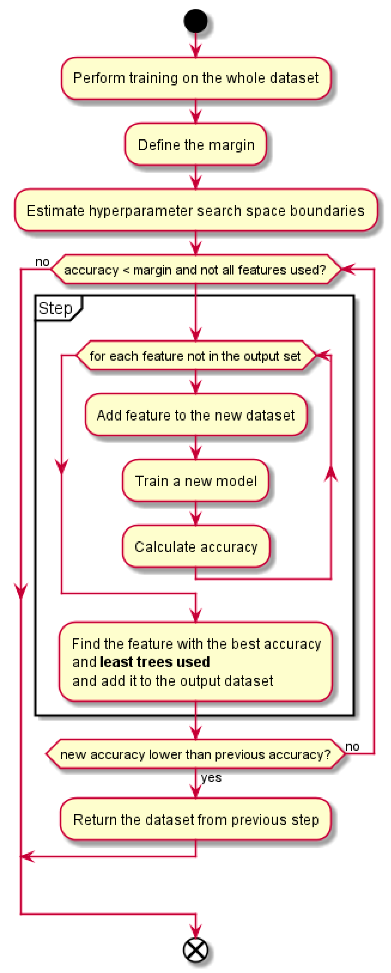
A block diagram of our proposed method is presented in the Figure 1. First three blocks serve as the preparation phase: training of the classifier on the whole dataset, defining the margin that defines the terminating condition for the main loop and estimation of the hyperparameter search space size. Then, in the main loop, at each repetition (“Step”), all the features are used for training and the feature that yields the best prediction quality is selected for inclusion into the output dataset. The main loop ends when the achieved prediction quality reaches the margin. More detailed description of the algorithm follows in the Section 2.4.

Key contributions of our work consist of:

• Evaluation of prominent existing ways of obtaining feature importances with RF models. These are found to be inadequate for multicollinear data.
• Proposal of a greedy forward feature selection method based on feature importance with a least-trees-used optimization.
• Verification of the proposed method using two real-world datasets that are widely used in the scientific community. It will be shown that the proposed method successfully selects small number of most important features and these are sufficient to build a model that yields an accuracy comparable to accuracy of a model built from the complete initial dataset.

In this paper, we first describe used tools, data and both existing and newly proposed algorithms in Section 2. In Section 3, we present results of our experiments using the new proposed algorithm. At the end, we sum up our findings and envision further use of our proposed method on the data not presented here in Section 4.

2. Materials and Methods

2.1. Tools

Experiments were carried out in the Python language using the popular scikit-learn package [18]. We concentrated on classification problems only. Training the RandomForestClassifier estimators was done using the utility GridSearchCV function which performs k-fold cross-validation and at the same time, a search over hyperparameter space. The RF classifier can use out-of-bag training method, and in this case cross-validation is not needed (as stated in [9]). So we implemented a special “cross-validation” method that takes a complete input dataset (n_splits = 1) and performs only the hyperparameter space search (see [19]). The out-of-bag mode of operation was enabled by setting classifier’s oob_score parameter to 1. After the training, the trained best estimator and all its parameters are retained in the GridSearchCV function’s output data structure.

We denote with X a matrix of input samples with N samples as rows and P features as columns. Vector of sample labels is denoted with y and the classifier output vector (predictions) with y_pred.

With RF, the hyperparameter space search can be performed on two hyperparameters: max_features and n_estimators. The former limits the number of features used in the formation of branches in the trees and the latter limits the number of trees trained. The values searched were {2ⁱ; i = {0, 1, 2, …, floor(log₂ P)}, P} for max_features and {i²; a < = i < = b} for n_estimators. The search rule for the max_features parameter was set up in accordance with the RF authors’ recommendation (they denote it mtry0) [20]. The limits a and b were estimated for each dataset as follows. Initial values were chosen based on previous experiments on the same datasets to: a = 1; b = 4. Then experiments were performed and the limit b was increased by one until the best accuracy was obtained using the value of n_estimators strictly below the upper limit b². The lower limit a was subsequently raised if values of the n_estimators parameter were consistently higher than previous values of a². Values of the limits a and b estimated in this way were 4 and 11 for the first dataset and 1 and 6 for the second one. Such sparse hyperparameter values were chosen to reduce search time. The best value for the max_features hyperparameter was later determined to be 1 in all of the experiments we performed.

As the prediction quality criterion, the accuracy was used which is defined as average of equal values of predictions vs. true outputs over all samples (where δ denotes Kronecker delta function):

Acc = E(δ(y_pred, y)).

(1)

We defined the margin ε as a termination criterion of the algorithm as one half of one sample and the goal accuracy margin Acc_ε as:

ε = (0.5/N) × Acc₀
Acc_ε = (1 − (0.5/N)) × Acc₀

(2)

2.2. Data

In the experiments, we used two datasets that are widely used in the research community. The first one is a modified dataset from the KDD Cup 1999 competition, called NSL-KDD dataset (after the Network Security Laboratory of University of New Brunswick, Canada), which is commonly used in training of the computer networks’ intrusion detection system models [21]. We only used its full training set contained in the KDDTrain+.arff file. It consists of 125,973 samples with 41 features and has a modest multicollinearity. The samples are labelled either ‘normal’ or ‘anomaly’. It can be obtained from several online sources, e.g., [22]. The other one is UCI Breast Cancer Wisconsin Dataset (later referred to as UCI-BCW dataset) with bigger multicollinearity. It consists of 569 samples with 30 features. The samples are labelled either ‘malignant’ or ‘benign’. This dataset can be obtained through a call to the scikit-learn library function load_breast_cancer.

A measure of rank collinearity M of a given dataset can be defined as a mean of absolute values of Spearman’s rank correlation coefficients ρ of all distinct feature pairs:

M = E(|ρ_ij|); i = {1, …, N}, j = {i + 1, …, N}, j ≠ i.

(3)

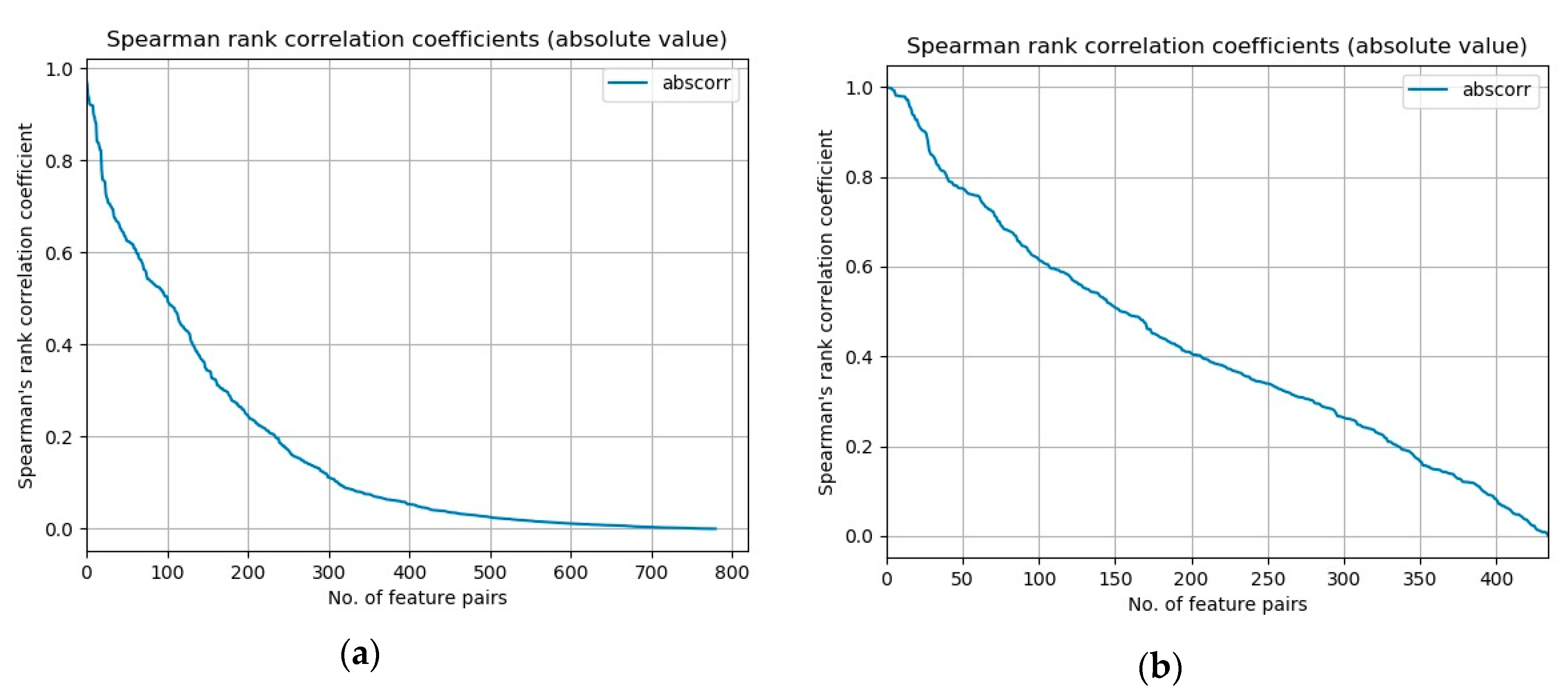
Values of measure M for our datasets are 0.172 for the NSL-KDD dataset and 0.422 for the UCI-BCW dataset. Another informative representation of this measure is a graphical one. Figure 2 presents plots of absolute values of Spearman’s rank correlation coefficients of all distinct feature pairs for both datasets, ordered by their absolute value in descending order. We can see that in the case of UCI-BCW dataset, the coefficients’ absolute values decrease slower from their maximum value on the left to the minimum on the right, than in the NSL-KDD case.

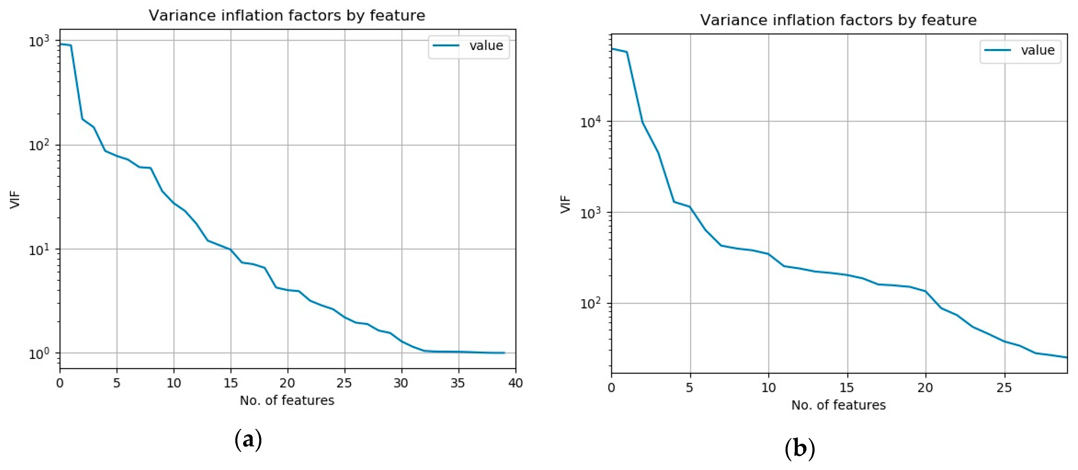
As a measure of multicollinearity, the variable inflation factor (VIF) is commonly used [2]. It expresses the degree to which a given feature can be predicted from all the other features of the dataset. We have computed it for all the features of both our datasets and plotted them again ordered from the largest to the smallest, which is presented in the Figure 3.

Mean values of VIF for the NSL-KDD dataset is 67.22 whereas for the UCI-BCW dataset it is much larger: 4749.56. It is known that VIF values above 5 or 10 indicate a presence of multicollinearity. So we can see that these datasets contain a substantial multicollinearity and the UCI-BCW more than the other.

Given that RF is non-linear ML method and that VIF is calculated using a linear ML method (R²) it is an open research question if VIF is adequate in determining the suitability of RF methods.

2.3. Existing Algorithms

The scikit-learn RF built-in method for estimation of feature importances gave unreliable results on both datasets. Across different runs, this method assigned quite different values of importances to the features so that even their order was not consistent. The first three most important features along with their importance measures are shown in the

Table 1. The three most important features and their importance—NSL-KDD dataset, 10 runs. Each row contains the three most important features from a single run with their respective importance values for the built-in method.

1st Feature	Imp.	2nd Feature	Imp.	3rd Feature	Imp.
dst_bytes	0.111	same_srv_rate	0.059	service	0.056
dst_bytes	0.095	diff_srv_rate	0.092	src_bytes	0.082
dst_bytes	0.112	dst_host_same_srv_rate	0.099	diff_srv_rate	0.080
dst_bytes	0.120	src_bytes	0.098	dst_host_same_srv_rate	0.079
src_bytes	0.091	dst_host_same_srv_rate	0.078	dst_bytes	0.073
src_bytes	0.102	dst_host_same_srv_rate	0.072	flag	0.066
src_bytes	0.126	same_srv_rate	0.093	serror_rate	0.084
src_bytes	0.066	dst_host_serror_rate	0.064	dst_bytes	0.063
src_bytes	0.090	dst_bytes	0.079	same_srv_rate	0.079
dst_bytes	0.109	src_bytes	0.088	dst_host_srv_count	0.077

and summarized in the

Table 2. The most frequent feature combinations by importance order—NSL-KDD dataset, 10 runs. For each importance level, the features that were placed to that level are listed with the percentages of their occurrence at that level among runs for the built-in method.

Importance Level	Feature	Frequency (%)
1	dst_bytes	50
1	src_bytes	50
2	dst_host_same_srv_rate	30
2	same_srv_rate	20
2	src_bytes	20
2	diff_srv_rate	10
2	dst_host_serror_rate	10
2	dst_bytes	10
3	dst_bytes	20
3	src_bytes	10
3	service	10
3	diff_srv_rate	10
3	dst_host_same_srv_rate	10
3	flag	10
3	serror_rate	10
3	same_srv_rate	10
3	srv_count	10
…

for the NSL-KDD dataset and likewise in the

Table 3. The three most important features and their importance—UCI-BCW dataset, 20 runs. Each row contains the three most important features from a single run with their respective importance values for the built-in method.

1st Feature	Imp.	2nd Feature	Imp.	3rd Feature	Imp.
worst area	0.104	mean compactness	0.087	worst radius	0.086
mean concave points	0.120	mean radius	0.109	mean concavity	0.075
mean concave points	0.149	worst area	0.084	worst perimeter	0.074
mean concave points	0.147	mean perimeter	0.109	mean concavity	0.093
worst radius	0.130	area error	0.116	worst concave points	0.097
worst concave points	0.123	mean perimeter	0.096	area error	0.070
worst concavity	0.079	mean area	0.073	mean concave points	0.070
worst area	0.140	worst perimeter	0.129	area error	0.113
worst perimeter	0.135	worst area	0.094	mean radius	0.089
worst area	0.088	mean area	0.087	mean concave points	0.075
worst perimeter	0.162	mean perimeter	0.151	mean concave points	0.080
mean concavity	0.130	mean concave points	0.122	worst area	0.115
mean concave points	0.096	worst concave points	0.074	mean radius	0.071
worst radius	0.125	worst area	0.082	mean concave points	0.079
worst perimeter	0.176	mean concavity	0.062	worst compactness	0.059
worst perimeter	0.132	worst radius	0.114	mean concave points	0.076
worst concave points	0.079	mean concave points	0.073	mean perimeter	0.070
worst perimeter	0.081	worst radius	0.073	area error	0.072
mean radius	0.107	worst perimeter	0.099	worst area	0.083
mean perimeter	0.101	worst perimeter	0.088	worst radius	0.066

and

Table 4. The most frequent feature combinations by importance order—UCI-BCW dataset, 20 runs. For each importance level, the features that were placed to that level are listed with the percentages of their occurrence at that level among runs for the built-in method.

Importance Level	Feature	Frequency (%)
1	worst perimeter	25
1	mean concave points	20
1	worst area	15
1	worst concave points	10
1	worst radius	10
1	mean concavity	5
1	mean perimeter	5
1	mean radius	5
1	worst concavity	5
2	worst area	15
2	worst perimeter	15
2	mean perimeter	15
2	mean area	10
2	mean concave points	10
2	worst radius	10
2	area error	5
2	worst concave points	5
2	mean compactness	5
2	mean concavity	5
2	mean radius	5
3	mean concave points	25
3	area error	15
3	mean concavity	10
3	mean radius	10
3	worst area	10
3	worst radius	10
3	mean perimeter	5
3	worst compactness	5
3	worst concave points	5
3	worst perimeter	5
…

for the UCI-BCW dataset.

The experiments with the package rfpimp [16] using its methods of permutation feature importance and drop-column feature importance gave similarly unreliable results. On the less multicollinear NSL-KDD dataset, the only consistent result was that the src_bytes was the most important feature. All the other features appeared on the list of the most important features randomly, even sometimes with zero importance, while at other runs with non-zero one. On the more multicollinear UCI-BCW dataset, no feature was consistently placed at the top.

All the importance measure values obtained from the rfpimp methods were very low. They were consistently below 0.01, which is far lower than the sensible lower limit of 0.15 recommended by the package authors.

These results show that usual methods of determining the most important features are inadequate to support the task of feature selection in cases where the data exhibit stronger multicollinearity. The main problem here is a lack of consistency of the results. If, according to these methods, several features were designated as most important in different runs then we might need to include all of them in the final dataset to avoid loss of information. This would make the feature selection process less efficient.

These shortcomings of existing methods prompted us to find a new method of defining feature importance in the multicollinear settings.

2.4. Proposed Algorithm

The proposed greedy feature selection algorithm is defined as follows. We start with a RF model, pre-trained on the dataset at hand. This model serves only as a baseline for determining an end criterion later in the procedure. Then we take an empty output dataset and successively add individual features from the original dataset that yield the best prediction quality. In the first step, when the output dataset is empty, we try each of the feature alone and get their individual prediction quality. The feature with the best prediction quality is added to the output dataset. In the second step, all the remaining features are evaluated along with the one chosen in the first step and the best quality feature in this combination is added to the output dataset. An important part of the procedure is that a new model is trained for each evaluated feature, including the hyperparameter search. This procedure of adding the best quality feature to the output dataset is repeated until the prediction quality of the new model is lower than the prediction quality of the original model only for a predefined small value ε. In the datasets with a large multicollinearity, the number of necessary steps proves to be quite low. Therefore, the number of necessary training runs is acceptable. Pseudo-code for this procedure is shown in Algorithm 1.

The hyperparameter space search is performed every time a feature is evaluated for inclusion to the output dataset. It turns out that if we omit this step, the results can be numerically unstable. With this step included, the best prediction quality is achieved and so the most informative feature is selected.

Algorithm 1 Greedy Feature Selection.
1	Train a model on input dataset and remember its accuracy
2	Define ε, margin = Accε
3	Define empty output set of features
4	Estimate hyperparameter search space for the given dataset
5	Repeat until the best accuracy ≥ margin or all features are used {
6	For each feature not in the output set {
7	Make temporary feature set from output set plus the current feature
8	Train the model with hyperparameter search using temporary feature set
9	Obtain predictions from the newly trained model
10	Calculate prediction accuracy
11	}
12	Find the temporary feature set with the best accuracy and least trees used
13	Make the temporary feature set found in the previous line the new output set
14	If the best accuracy from the current step is less than the one from the previous step {
15	Finish the loop and make the output dataset the one from previous step
16	}
17	}
18	Return the output dataset

We refer to the block of lines 6–16 in the Algorithm 1 as a “step”. A step finds a feature to be added to the output dataset by using the criterion of the best accuracy and least trees used. The line 12 consists of the important part, which is the least-trees-used criterion and this is a key novelty of our method.

Often, multiple features achieved the same accuracy at some step in our experiments. The final choice among them (line 12 in Algorithm 1) was then performed in two ways: the first way was using the first or random one, and the second way was using the feature that was modelled by means of the lowest number of trees. As it is confirmed in the results section, the least-trees-used approach proved to be better.

This algorithm is theoretically not guaranteed to converge. It is, theoretically, possible to reach a local maximum that is dealt with by the exit condition of the line 14 if the new accuracy is less than the accuracy from the previous step. If the algorithm does not end up in a local maximum then it finishes at least when coming to use all the input features, for which we have obtained a working model beforehand. In all our experiments with the two given datasets, the algorithm concluded a lot earlier, by using only a small subset of features.

Random Forests calculates the feature importance values in the process of building the trees and in the scikit-learn implementation provides them as an output property feature_importances_ of a trained RandomForestRegressor or RandomForestClassifier object. Feature selection based on these values commonly consists of sorting the features by their importance and eliminating some number of the least important ones. In the proposed algorithm, the process is reversed so that we gradually add features to the new dataset and the basic criterion to include them is the best accuracy.

Commonly, the feature selection process based on the feature importances ends after some predefined number of features is eliminated. This principle is implemented, e.g., in the popular helper functions RFE and RFECV in the scikit-learn Python package. In the proposed algorithm, a different principle is implemented so that it terminates the feature selection process after a sufficiently high accuracy is achieved.

The algorithm and an application to use it are deposited at the public repository https://github.com/fdrobnic/GFS.

3. Results

Initial accuracy of models trained on the original datasets Acc₀ was on average 0.9999398 with σ = 6.84 × 10⁻⁶ in 10 runs for the NSL-KDD dataset and 0.99895 with σ = 0.00149 in 20 runs for the UCI-BCW dataset.

The exact run times were not part of our research interest, but we made a rough estimation of the computing time until the goal accuracy was achieved using the given computer resources. Total computing time until the goal accuracy was achieved was on average 12 h 39 min 28 s with σ = 2 h 50 min 12 s in 10 runs for the NSL-KDD dataset and on average 5 min 51 s with σ = 19 s in 20 runs for the UCI-BCW dataset. The experiments were performed on a laptop with four core CPU with a clock speed of 3 GHz. Parallel processing during training and prediction was employed by setting the classifier and the GridSearchCV function parameter n_jobs to -1, which means to use all available CPU cores. Such computing time implies that our proposed method of feature selection is not suitable to be performed in real time. Nevertheless, this seemingly large consumed time can pay off in lowered processing and communication costs in the aforementioned use case of IoT. We consider such amount of time not too high for a one-time process of finding most informative features, which was our primary goal. A possibility for reducing the computing time would be using a smaller sample of the data, especially from the NSL-KDD dataset. On the other side, the computing time of predictions on the whole datasets used to find the accuracy of these models was substantially shorter, it was 0.30 ± 0.05 s for the NSL-KDD dataset and 0.117 ± 0.001 s for the UCI-BCW dataset. There was no significant difference between computing times on the whole datasets compared to computing times on the reduced datasets, possibly because Python is an interpreted language and the runtime overhead contributes the majority of the time consumed.

Accuracy improvement due to choosing the feature that was modelled at the step 11 of Algorithm 1 using the least trees was substantial, especially in the case of the UCI-BCW dataset. By choosing one of equally good features at random (or simply the first one) the average accuracy was 0.99584 with σ = 0.00407 and with the least-trees-used optimization it was 0.99877 with σ = 0.00168 which is nearly as good as the initial accuracy on the whole dataset. The results with the least-trees-used option were also more consistent, at least at the first step. In both cases, the most probable feature at the first step was “mean concave points”. With the first option, it was chosen in 66.67% of runs and with the second option in 95% of all runs. In the case of the NSL-KDD dataset, the difference between qualities of both options was smaller, but also in favour of the least-trees-used option. The criterion of the least trees used can be regarded as a form of “regularization” that prevents the model to adhere to the training dataset too strictly [23] (p. 596). We have therefore chosen the least-used-trees option, and only the results obtained from the least-used-trees option will be evaluated.

Even with hyperparameter search after each feature addition, the selected features were different among runs. The

Table 5. The most frequent feature combinations—NSL-KDD dataset, 10 runs. For each step, the features that were selected at that step are listed with the percentages of their occurrences at that step among runs for the newly proposed method.

Step	Feature	Frequency (%)
1	src_bytes	100
2	dst_host_same_srv_rate	100
3	service	100
4	count	100
5	dst_host_srv_count	100
6	flag	70
6	dst_host_diff_srv_rate	30
7	dst_bytes	80
7	dst_host_count	10
7	rerror_rate	10
8	dst_host_srv_diff_host_rate	40
8	dst_host_srv_serror_rate	20
8	hot	10
8	land	10
8	protocol_type	10
8	srv_count	10
9	dst_host_srv_diff_host_rate	30
9	dst_host_srv_serror_rate	30
9	duration	10
9	num_access_files	10
9	num_failed_logins	10
9	protocol_type	10
10	dst_host_srv_diff_host_rate	30
10	dst_bytes	10
10	dst_host_diff_srv_rate	10
10	dst_host_srv_serror_rate	10
10	land	10
10	num_failed_logins	10
11	dst_host_srv_serror_rate	30
11	num_shells	10
12	dst_host_same_src_port_rate	10
12	num_outbound_cmds	10
13	dst_host_srv_serror_rate	10

and

Table 6. The most frequent feature combinations—UCI-BCW dataset, 20 runs. For each step, the features that were selected at that step are listed with the percentages of their occurrences at that step among runs for the newly proposed method.

Step	Feature	Frequency (%)
1	mean concave points	95
1	mean concavity	5
2	radius error	15
2	mean area	10
2	symmetry error	10
2	worst area	10
2	worst radius	10
2	worst texture	10
2	compactness error	5
2	concave points error	5
2	mean perimeter	5
2	mean radius	5
2	mean symmetry	5
2	perimeter error	5
2	worst compactness	5

summarize the most common feature combinations from the NSL-KDD and the UCI-BCW dataset, respectively. Variations in selection of a feature at some step is indicated with multiple features present in the row of that step and percentage of runs where that feature was selected.

Note that different runs reached the goal in different number of steps for the NSL-KDD dataset (this is indicated in the sum of percentages not giving 100% for the steps 10 and above). Two examples of the shortest chains are shown in the

Table 7. The smallest feature combinations—NSL-KDD dataset. For each step, the features that were selected at that step in two shortest runs are listed for the newly proposed method. Note the equality of selected features in several steps.

Step	One of the Runs	Equal?	Another Run
1	src_bytes	=	src_bytes
2	dst_host_same_srv_rate	=	dst_host_same_srv_rate
3	service	=	service
4	count	=	count
5	dst_host_srv_count	=	dst_host_srv_count
6	flag		dst_host_diff_srv_rate
7	dst_bytes	=	dst_bytes
8	dst_host_srv_serror_rate		dst_host_srv_diff_host_rate
9	dst_host_srv_diff_host_rate		dst_host_srv_serror_rate

.

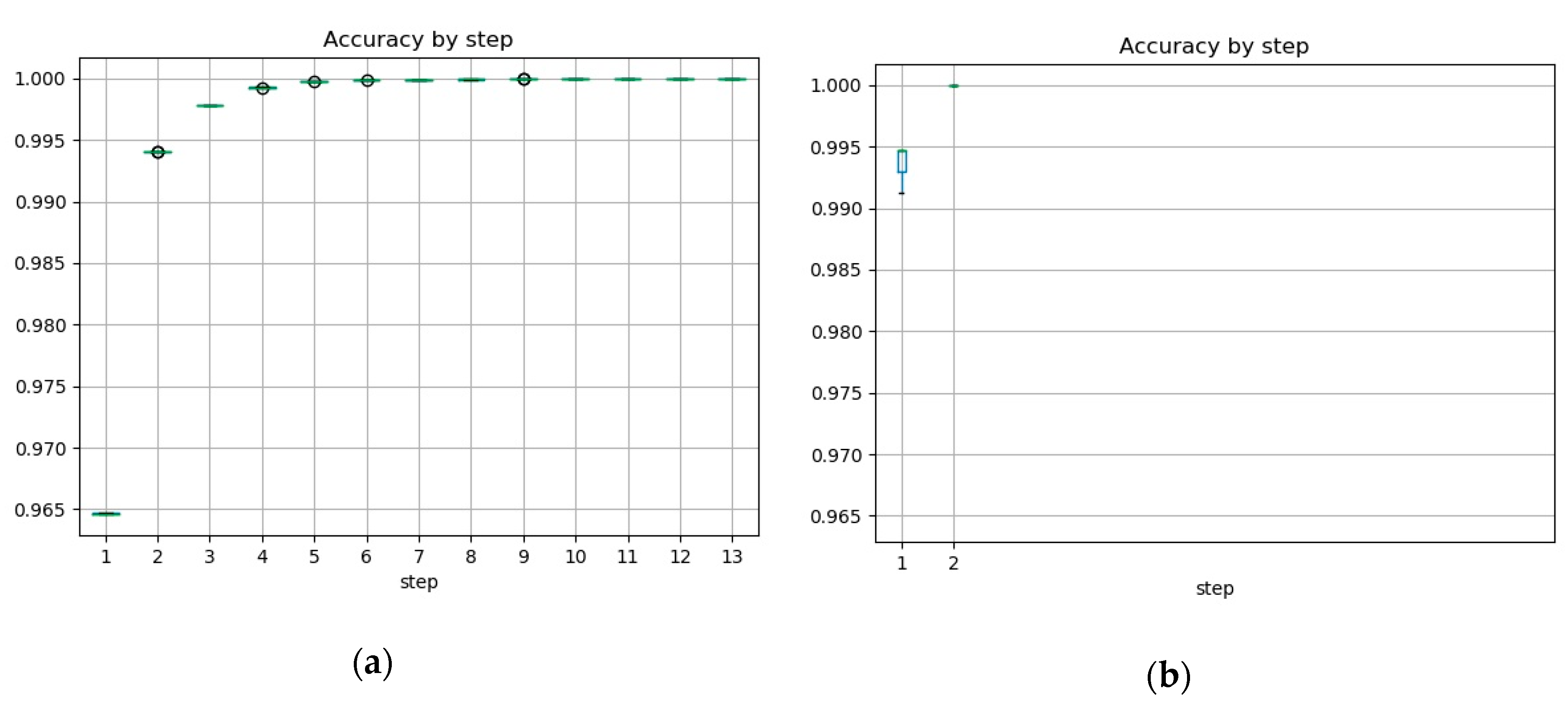
At every step, accuracy of the trained model increased and finally reached the goal accuracy, as presented by boxplots in Figure 4 for each of two datasets. It is clearly visible that the less multicollinear dataset needed more steps to achieve the goal accuracy and started from a lower accuracy than the more multicollinear one.

It is true that, even with the least-trees-used criterion implemented, there were cases where the same minimum number of used trees was achieved with more than one feature. In this case, it would be possible that a domain expert would choose among those features based on knowledge not known to us. It could be facilitated by extending our software to provide a user with such choice in the course of model training, which is known as the human-in-the-loop approach.

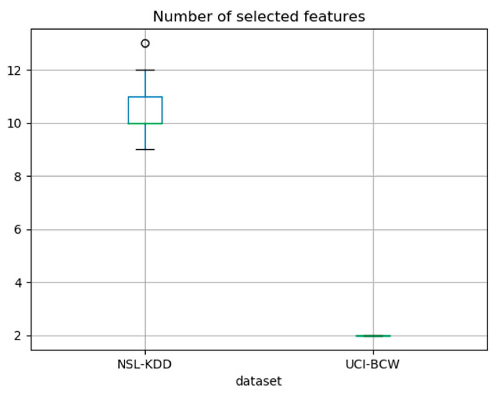
In case of the NSL-KDD dataset, number of selected features was varying among runs from nine to 13, whereas in case of UCI_BCW dataset, it was consistently two. The Figure 5 displays these numbers as a pair of boxplots to provide a statistical information about them.

We have, thus, verified that the proposed greedy forward feature selection method with least-trees-used criterion does indeed achieve the imposed goal. It does find a consistent subset of input features that can be used in training a model and obtaining that model’s predictions with an accuracy, which is almost as high as the initial accuracy of a model trained on the complete dataset and is lower than that only for a small margin ε.

4. Conclusions

The greedy forward feature selection algorithm with least-trees-used criterion for use in highly multicollinear datasets is proposed and tested on two benchmark datasets, which are widely used in the scientific community. Their multicollinearity was determined using pairwise Spearman’s rank correlation coefficients on the features and using the standard multicollinearity measure—variable inflation factor (VIF). Both measures showed that both datasets are multicollinear and that the UCI-BCW dataset is more multicollinear than the NSL-KDD dataset.

We have shown that it is possible to find the most important features even in datasets with a high multicollinearity where existing methods do not give consistent results. Our method achieves better results with more multicollinear datasets. In the case of the NSL-KDD dataset, the necessary number of steps and thus the number of selected features was from nine to thirteen, whereas in the case of the more multicollinear UCI-BCW dataset, this number was only two. We were in both cases able to perform predictions using such reduced feature set with an accuracy comparable to that of the complete initial dataset. Note that the primary goal of our research was not like classical ML problems of achieving as good prediction quality as possible, but instead to perform a feature selection, which would give such feature subset that would support similar prediction quality as the original dataset. The feature selection process consumes some computing time. It is, however, performed once and in advance so that the reduced model can be built, which then potentially uses less processing power and less communication in the prediction phase of its lifecycle, when it may perform a lot of predictions.

Because in the process we build new models, our method serves more to the purpose of finding most informative features from a given dataset rather than that of explanation of existing model predictions. However, in this way we can understand what features can drive any model due to quantity of information they can provide with regard to the predicted variables.

The method could be improved further by implementing a human-in-the-loop approach where domain expert would assist in choosing the most appropriate feature from a subset of equally performing features, based on the domain knowledge.

We initially developed and tested the algorithm for the feature selection stage during modelling of the influence of bio-psycho-social features of children and adolescents on their motor efficiency. The preliminary test results were promising. As the algorithm proved to be excellent for multicollinear datasets, we generalized it and now we present it in this article in its generic form. We expect it to become an important tool for the scientific community.

The proposed algorithm is not limited to any domain, as long as supervised machine learning environment is provided. It means that the records of the training dataset are labelled with class labels.

We published the software that can be used to reproduce the results presented here on the public repository: https://github.com/fdrobnic/GFS.