Channel and Spatial Attention Regression Network for Cup-to-Disc Ratio Estimation

Abstract

Cup-to-disc ratio (CDR) is of great importance during assessing structural changes at the optic nerve head (ONH) and diagnosis of glaucoma. While most efforts have been put on acquiring the CDR number through CNN-based segmentation algorithms followed by the calculation of CDR, these methods usually only focus on the features in the convolution kernel, which is, after all, the operation of the local region, ignoring the contribution of rich global features (such as distant pixels) to the current features. In this paper, a new end-to-end channel and spatial attention regression deep learning network is proposed to deduces CDR number from the regression perspective and combine the self-attention mechanism with the regression network. Our network consists of four modules: the feature extraction module to extract deep features expressing the complicated pattern of optic disc (OD) and optic cup (OC), the attention module including the channel attention block (CAB) and the spatial attention block (SAB) to improve feature representation by aggregating long-range contextual information, the regression module to deduce CDR number directly, and the segmentation-auxiliary module to focus the model’s attention on the relevant features instead of the background region. Especially, the CAB selects relatively important feature maps in channel dimension, shifting the emphasis on the OD and OC region; meanwhile, the SAB learns the discriminative ability of feature representation at pixel level by capturing the relationship of intra-feature map. The experimental results of ORIGA dataset show that our method obtains absolute CDR error of 0.067 and the Pearson’s correlation coefficient of 0.694 in estimating CDR and our method has a great potential in predicting the CDR number.

1. Introduction

As the second leading cause of blindness, glaucoma is a disease that causes damage to the optic nerve of the eyes resulting in deteriorated vision [1]. Once diagnosed, the disease cannot be treated completely, but timely detection can further control the effect of glaucoma. Therefore, early detection and treatment are essential for glaucoma patients to safeguard their vision [2,3,4].

Various diagnosis parameters of glaucoma are proposed, such as CDR, ISNT rule, DDLS, GRI (Glaucoma risk index) [5], which are used for assessing structural changes at the optic nerve head (ONH) and diagnosis of glaucoma. The CDR is widely regarded as one of the crucial indications of the risk factor for diagnosis of glaucoma. It is calculated by the ratio of vertical cup diameter (VCD) to vertical disc diameter (VDD). Calculation of the CDR includes subjective assessment by observing fundus photographs, or interactive segmentation tools which allow clinicians for manual segmentation and grading, such as DCSeg (specifically designed to manually segment the optic disc and cup.) [6]. There is no denying that these traditional processes are labor-intensive, time-consuming and costly.

Automatic diagnosing glaucoma can eliminate the above shortcomings, such as a computer-aided diagnosis system [7,8,9]. Two categories of solutions exist for automatic diagnosing glaucoma using CDR: segmentation methods and direct estimation methods. The former takes segmentation masks as network output. To get an accurate measurement of CDR, precise segmentation of OD and OC is needed. it is surprisingly difficult to obtain excellent and robust segmentation owning to the existence of a lot of vessels traversing the OC’s boundary, diverse structural changes and the differences between subjects. The latter without segmentation usually deduces the CDR number directly, which has grown in popularity and has satisfactory performance. Distinguished from most previous work that relies on the premise of joint OD and OC segmentation, we address the problems as a regression task using deep learning technology.

CNN has demonstrated high power in a board range of computer vision, as well as medical image analysis. Some algorithms [10,11] are designed, such as U-net to generate the segmentation masks directly. The standard U-net, nevertheless, only concentrates on local features, which cannot consider the large-range contextual information effectively.

For this task to get accurate CDR numbers, distinguishing blurred OD and OC boundaries must be within our considerations. For example, the cup boundaries are more indistinguishable from the disc boundaries, at the same time, a lot of vessels traversing the OC’s boundary and background region will affect the precision of the task. Therefore, it is crucial to improve the discrimination ability of each pixel’s representation. M-net [12] uses the multi-scale to solve this unanswered question.

Different from previous work, in this paper we propose a novel and effective combination model, which effectively combines self-attention mechanisms with the regression network to solve the problem mentioned above.

Here, our proposed self-attention mechanism consists of channel attention block (CAB) and spatial attention block (SAB), which is added to the middle of traditional U-net. The CAB selects relatively important feature maps in channel dimension, shifting the emphasis on the OD and OC region. Meanwhile, the SAB learns the discriminative ability of feature representation at the pixel level by capturing the relationship of the intra-feature map. Through experiments, we also find that the SAB makes the classification of pixels on the boundary area more accurate. Then, a fusion operation is used to combine the two blocks into one. Finally, the CDR number is predicted by convolutional layers.

Another challenge is that the deep learning regression module is like a black box, and it is tough to select features that could represent OD and OC accurately. However, it is easy to learn some features or focus on a specific region (such as OC, OD) for the segmentation task, but these features are difficult to learn via the single regression task. Therefore, the segmentation-auxiliary module (SAM) is introduced into our model, which is parallel to the main regression task. Intuitively it can focus the model’s attention on the relevant features instead of the background region. In this way, during the test, our model works in an implicit way for which image segmentation information is considered but not displayed.

In summary, proposed channel and spatial attention regression model (CSAR) consists of four modules as shown in Figure 1. The CSAR contains the feature extraction module to extract deep features expressing the complicated pattern of OD and OC, the attention module to improve feature representation by aggregating long-range contextual information, the regression module to deduce a CDR number directly, and the segmentation-auxiliary module to focus the model’s attention on the relevant features instead of the background region. The main contributions of our paper include:

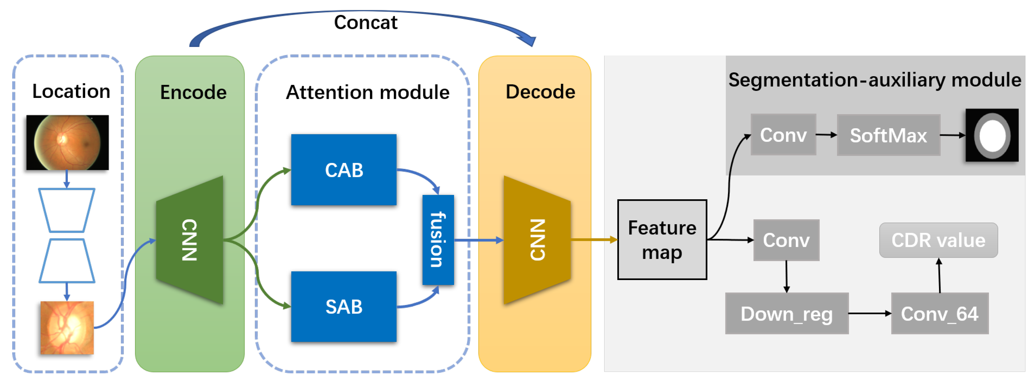
• We propose an end-to-end channel and spatial attention regression deep learning network for predicting CDR, which jointly learns the self-attention module and the regression module.
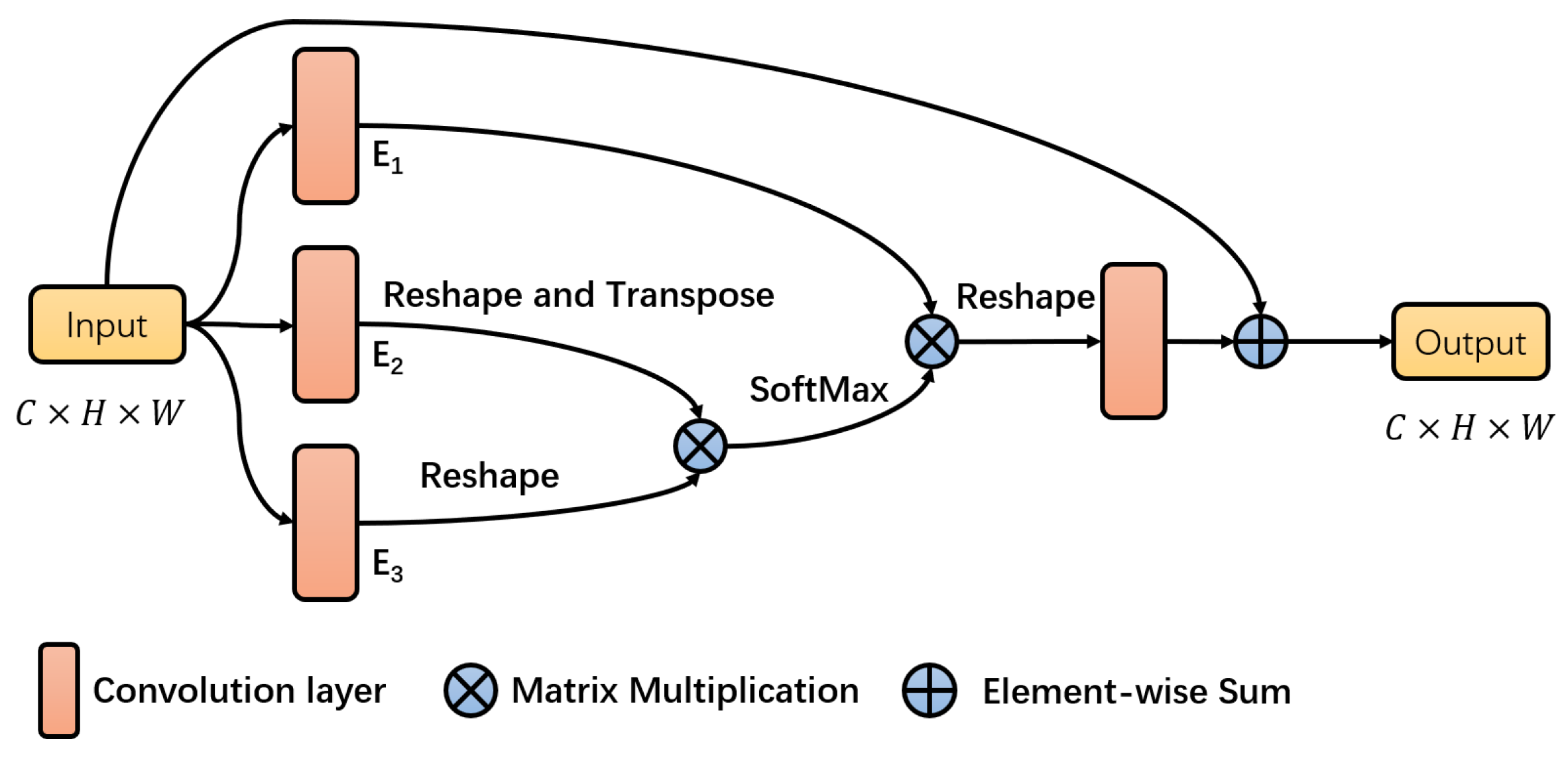
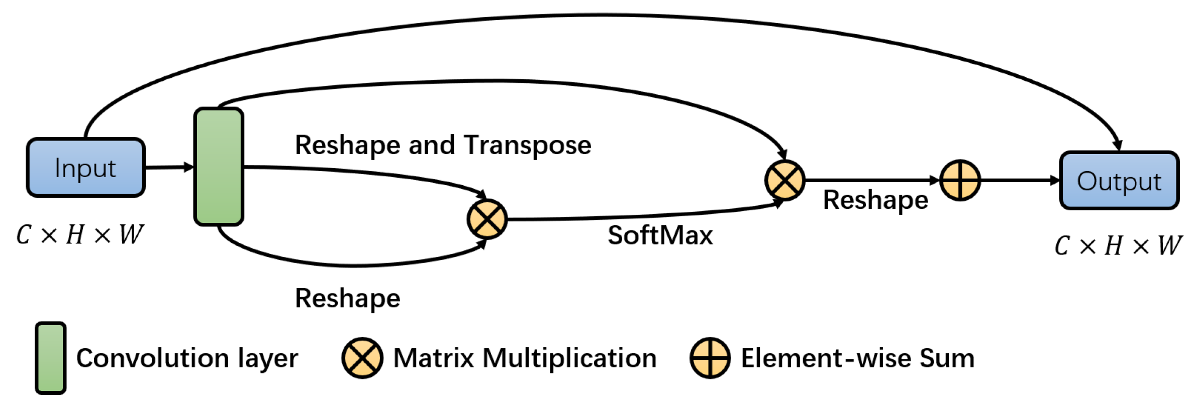
• Proposed channel attention block can select relatively important feature maps in channel dimension, shifting the emphasis on the feature map that is closely related to the optic disc and cup region, and proposed spatial attention block can capture the relationship of the intra-feature map to improve the discriminative ability of feature representation at pixel level.
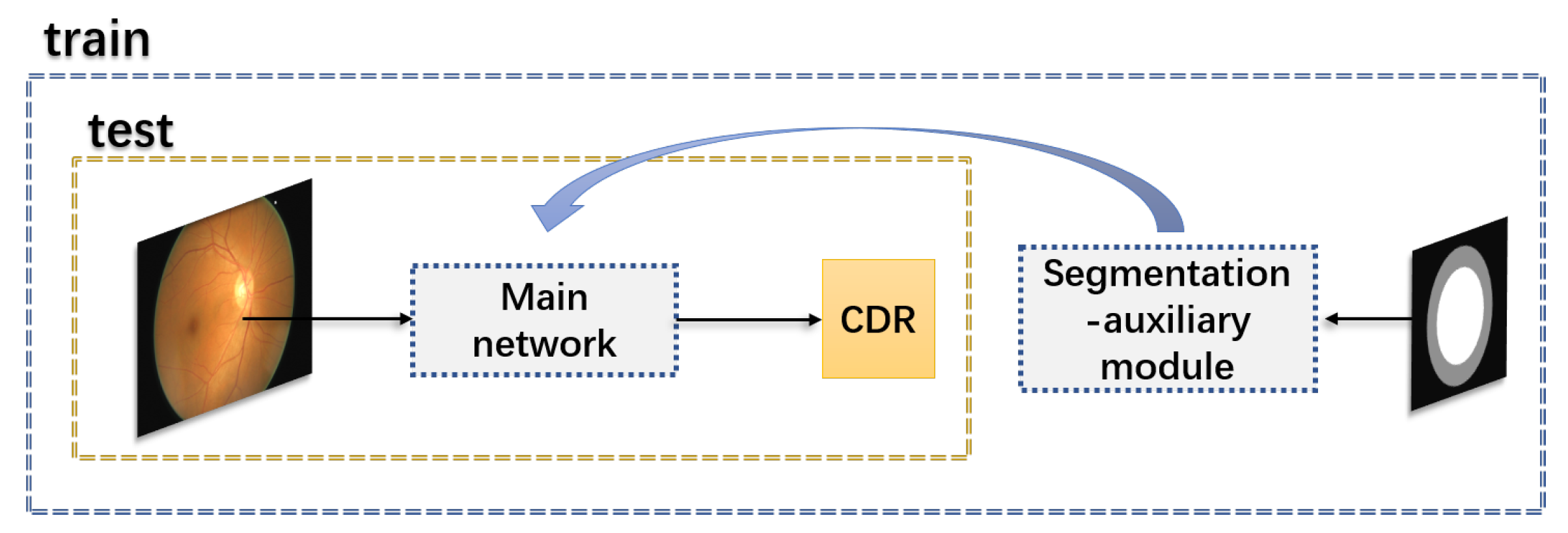
• We design a segmentation-auxiliary task to help the regression task focus on the optic disc and cup region instead of non-optic disc and cup region.

The remaining of the paper is as follows. In Section 2, we briefly review some methods of calculation of CDR number and some networks that use attention mechanism. In Section 3 the architecture of the CSAR is presented. Then we give the dataset, experiment details, results and discussions in Section 4. Section 5 gives the conclusion.

2. Related Work

In this section, some methods of calculation of CDR number are briefly reviewed, and we also present some networks that use attention mechanism.

2.1. Existing Two Methods of the Calculation of CDR

Automatic diagnosing glaucoma algorithms have been recognized by more and more people, such as a computer-aided diagnosis system [7,13,14,15,16]. Some glaucoma detection methods use CDR from spectral domain optical coherence tomography (OCT) Images [17,18,19,20,21,22,23], and others are from fundus images. There are two categories of solutions existing for calculation of CDR number: segmentation methods and direct estimation methods.

• Segmentation methods. Most researchers focus their efforts on the segmentation methods, part of which tend to focus on OD and OC segmentation independently. For the perspective of only OD’s segmentation, hand-crafted features are inevitably required, such as image gradient information extracted by active contour model [24], the local texture features [25], the disparity features extracted from the stereo image [26], and a novel polar transform method [27]. OC segmentation is also highly dependent on hand-crafted visual features. However, because the OD and OC have a certain structural similarity and positional correlation, joint OD and OC segmentation approaches obtain better performance [28,29]. Zheng et al. [28] joint the OD and OC segmentation leveraging a graph-cut mechanism. A superpixel-level classifier [29] is utilized to provide robustness for segmenting OD and OC. Recently, deep learning techniques have an excellent performance in computer vision, which are also widely used to joint OD and OC segmentation. Sevastopolsky et al. [30] design a modification of the U-net convolutional neural network (CNN), but it still operates in two stages. Futhermore, based on U-net, Qin et al. [31] combine deformable convolution and create a novel architecture for segmentation of OD and OC. Subsequently, the residual network (ResNet) is introduced, and whether generative adversarial networks (GAN) is helpful for OD and OC segmentation is discussed in [32]. M-net [12] develops the one stage multi-scale mechanism and adopts polar transformation to shift the fundus images to the polar coordinate system. However, finding the center point of OD is inevitably required, and the workload is increased to some extent. Unsupervised domain adaptation for joint OD and OC segmentation over different retinal fundus image datasets is exploited in [33]. The work in [34] deals with the OD and OC by combining the GAN. The segmentation problem is addressed as an object problem [35].
• Direct estimation methods. Direct methods usually deduce the CDR numbers directly without segmented OD and OC. The existing method using machine learning has two stages: unsupervised feature representation with CNN and CDR number regression by random forest regressor separately [36].

2.2. Existing Attention Model

It is proved that the attention mechanism has been successfully adopted in CNN, significantly boosting the performance of many vision tasks [37,38,39,40]. Self-attention [41] is first proposed and applied in the domain of natural language processing (NLP). Recently it has also gained attention in the domain of computer vision [42,43,44,45]. The essence of the self-attention mechanism is to emphasize or select important information of target objects and suppress some irrelevant details through a series of attentional distribution coefficients, namely weight coefficients. The attention mechanism especially self-attention mechanism can flexibly capture the connection between local information and global information in one step, improving the model’s presentation ability. Moreover, small and light structure is another advantage of attention mechanism. In particular, the non-local network [42] computes the response at a position as a weighted sum of the features at all positions. Based on the covariance matrix of the non-local mechanism, Du et al. [43] design a new self-attention mechanism stimulated by PCA to generate attention maps, achieving better interaction. Woo et al. [44] put forward the spatial attention mechanism to distinguish the importance of different positions. To the best of our knowledge, few methods combine the attention model in the CNNs for glaucoma detection. Only one method [45] is proposed which introduces the ophthalmologist’s attention map into AG-CNN to remove the redundancy of the fundus image; however, a human attention map is inevitably required.

3. Methodology

In this section, we first present an overview of our CSAR model, then the architecture of two attention blocks is introduced. Next, we describe how to aggregate the segmentation-auxiliary module for the regression task, and the train loss is presented in the end.

3.1. Overview

Our model bases on traditional U-net and the general architecture of the model is as follows. Firstly, the encoder module contains four encoder blocks, and the residual network block is employed as the backbone for each block. After that, enter the attention mechanism: the channel attention block (CAB) and the spatial attention block (SAB). The structure of the self-attention mechanism is shown in Figure 2 and Figure 3. The purpose of CAB is to acquire the connection between different channels automatically. The parallel SAB takes effect on the connections within the pixel, weighting different regions in the one feature map to make the regression model focus on the relevant feature areas, highlighting the salient regions. The attention module proposed is the independent allocation of weights within and between feature maps, and the mechanism can be used for weight learning through backpropagation. Then, the decoder module symmetrically expands the path. Finally, feature maps flow into the segmentation-auxiliary module and regression module respectively, and the segmentation-auxiliary task transmits back the label information to guide the feature extraction. Similarly, the regression output is obtained by a CNN network. We note that our regression branch has a straightforward structure.

3.2. The Spatial Attention Block

From the global and local perspective, images often have different change rules. The cup and disc area and their shapes are focus of our attention. However, characteristics of the background area (such as blood vessels traversing the cup boundary) tend to cause some harm to the foreground (the OD and OC area); at the same time, the OC is inside the OD, which is essential position information that cannot be ignored.

In order to realize our observation, we propose the spatial attention block (SAB). The architecture of our proposed SAB is shown in Figure 2 and its function is: learn the discriminative ability of feature representation at the pixel level by capturing the relationship of the intra-feature map. The process can be divided into three parts: first, the weight matrix is generated according to the similarity degree between the pixels in the feature; second, the weight matrix and the original feature matrix multiplication; third, the matrix addition between the matrix obtained above and the input characteristics. To be specific: the input characteristics simultaneous feed into three convolution layers, attaining three new feature maps E1, E2, E3. After reshaping them, a matrix multiplication and SoftMax layer are performed between the transpose of E2 and E3, and attention map is acquired:

$$S_m^{ij}=\frac{exp(E_2^i·E_3^j)}{{\sum }_{i=1}^{H\times W}exp(E_2^i·E_3^j)}$$

(1)

where $S_m^{ij}$ marks the ith position’s impact on jth position.

For the feature at a particular position in one feature map, it is refreshed via aggregating feature at all pixels with weighted summation [46]. In short, any two existing similarity features can enhance each other’s expression. Features with more similar features (such as cups and plates) will be enhanced, and features with fewer similar features (such as blood vessels and background) will be less enhanced.

After that, we multiply the attention map and the transpose and reshape of E1, and then add the input feature I to redistribute the correlation information to the original feature map:

$$S_{final}^j={\lambda }_s\sum _{i=1}^{H\times W}(S_m^{ji}·E_1^i)+I^j$$

(2)

where a convolutional layer with kernel size 1 × 1 is set as a learnable parameter ${\lambda }_s$.

Through the above calculation, the attention map about the intre-feature map can well obtain the correlation between the global information and the location information and strengthen the closely similar features, thus solving the two problems we proposed.

3.3. The Channel Attention Block

Compared with the spatial attention block to capture global information, the channel attention block selects relatively important feature maps, shifting the emphasis on the optic disc and cup region.

Since each feature map in the channel dimension can be regarded as a class-specific corresponding [46], we use the interdependencies among channel maps to decompose the interdependent feature maps and improve some feature representations of specific semantics. In the field of glaucoma, there are usually several types of response: OD, OC, blood vessels, and other background areas. Through observation and experiments, however, it can be found that channel information of optic disc and cup accounts for a relatively large proportion, and there is a small amount of learned blood vessel information and other background areas. The weight matrix of channel similarity established by CAB can effectively enhance the corresponding degree of the cup and disc response.

The design of the CAB in Figure 3 is more similar to SAB. Unlike SAB which feeds input into three convolution layers, CAB only goes through one convolution layer, the process of calculating the weight matrix between features is similar, and the calculation formula is shown as:

$$C_m^{ij}=\frac{exp(F_2^i·F_3^j)}{{\sum }_{i=1}^{C}exp(F_2^i·F_3^j)}$$

(3)

where $C_m^{ij}$ marks the ith channel’s impact on jth channel. And $C_{final}^j$ with a size of $C\times H\times W$ is defined as:

$$C_{final}^j={\lambda }_c\sum _{i=1}^C(C_m^{ji}·F_1^i)+I^j$$

(4)

where a convolutional layer with kernel size 1 × 1 is set as a learnable parameter ${\lambda }_c$.

3.4. The Segmentation-Auxiliary Module

In general, the segmentation task and the regression task are carried out independently. However, mutual promotion can be achieved after the combination of the two tasks for the following reasons:

• Direct regression deep learning network is more like a black box, and we cannot understand which features are well mapped in the regression. Meanwhile, it is tough to select features that could represent the boundary of the optic cup and disc. The addition of the segmentation-auxiliary module makes the features about OD and OC have a specific prominent enhancement in the feature selection of the regression map. The experimental results prove that our conclusion is correct.
• The addition of the segmentation auxiliary module can improve the degree of network convergence.

The structure is shown in Figure 4: when getting the feature maps after the decode module, the model enters the segmentation-auxiliary path and the regression path. The segmentation label is obtained by a convolution layer and a SoftMax layer. Similarly, the final feature map in the decode module is passed through a convolution layer, then the final CDR number is acquired after three down-sampling layers and a convolution layer with kernel size 64 × 64.

The operation mechanism of our proposed networks is shown in Figure 4. Firstly, the training includes four parts: convolutional neural network for feature display, the dual-attention mechanism for enhancing the characteristics of OD and OC, and regression network supplemented by segmentation to help the regression optimization. In the test, the segmentation-auxiliary module is canceled, the result is only composed of regressed CDR number. Our model can provide a simple and convenient tool for doctors.

3.5. Training Loss

Segmentation loss. In segmentation branch, the Jaccard Index (intersection over union) is used and it means the intersection of two data sets divided by the union of two data sets, which is expressed as:

$$J(F_1,F_2)=\frac{|F_1\cap F_2|}{|F_1\cup F_2|}=\frac{|F_1\cap F_2|}{|F_1|+|F_2|-|F_1\cap F_2|}$$

(5)

From the pixel angle, the formula can be rewritten as follows:

$$J=\frac{1}{N}\sum _{i=1}^N(\frac{y_i\widehat{y_i}}{y_i+\widehat{y_i}-y_i\widehat{y_i}})$$

(6)

where $y_i$ represents the labels and $\widehat{y_i}$ represents the $i_{t}h$ predicted pixel. The final $L^s$ is expressed as follows:

$$L_s=H-log\left(J\right)$$

(7)

where H represents a categorical cross entropy.

Regression loss. During regression task, the mean square error is used to define the regression loss $L^r$, which is the sum of the squares of the differences between the predicted value and the target value.

Total loss. In the experiment, we first try to to add up the different losses simply. It soon becomes clear that although split tasks converge, regression task performs poorly. After further study, it is found that the scale between the two task losses is different, leading to the overall loss dominated by the first task. In order to balance the two tasks, we adopt the method in [47]. According to the two definitions above, like [47], the joint loss is expressed as follows:

$$L(\mathsf{\Theta },{\sigma }_1,{\sigma }_2)=\frac{1}{{\sigma }_1^2}\sum _{j=1}^N{L}_j^s+\frac{1}{{\sigma }_1^2}\sum _{j=1}^N{L}_j^r+log\left({\sigma }_1^2\right)+log\left({\sigma }_2^2\right)$$

(8)

where $\mathsf{\Theta }$ is a parameter, and the role of ${\sigma }_1$ and ${\sigma }_2$ is to balance the weight of two tasks and they are learnable in training. To be specific, the ultimate goal can be seen as learning the relative weight of each subtask output. In practice, to escape a potential division by zero, $\delta =log\left(\sigma \right)$ is redefined. Therefore, the final loss can be rewritten as:

$$L(W,{\delta }_1,{\delta }_2)=exp(-{\delta }_1)\sum _{j=1}^N{L}_j^s+exp(-{\delta }_2)\sum _{j=1}^N{L}_j^r+{\delta }_1+{\delta }_2$$

(9)

4. Experiments and Analysis

The effectiveness of our CSAR is verified in different aspects. Firstly, ablation study is used to test the performance of two attention blocks CAB and SAB for the regression network. Simultaneously we calculate the mean absolute error (MAE) and the correlation. Furthermore, the area under curve (AUC) is computed to evaluate our method on glaucoma screening. Then, by visualizing the attention map to verify our conclusions, the accuracy of the model can be improved more intuitively.

Secondly, to evaluate the segmentation-auxiliary module’s performance, the ablation study is also conducted by us. As described above, the experimental results with and without the segmentation-auxiliary module are still compared from three aspects: correlation coefficient, MAE and glaucoma screening accuracy. In addition, visualization of convolutional layers is presented to explain more clearly the problems that we encounter in the experiment.

Thirdly, we compare our CSAR to other traditional methods and deep learning methods, for example R-Bend [25], ASM [48], Superpixel [29], M-net [12], JointRCNN [35]. Our experiments still verify on the dataset ORIGA and use the same criteria. Finally, in this experiment, we also discuss and evaluate the ISNT rules.

4.1. Datasets and Configurations

The ORIGA dataset contains 650 fundus images with 482 normal eyes and 168 glaucomatous eyes. The set A including 325 images is used for training and the set B is used for testing [49]. In our experiment, the same division of the dataset is used as same as [12]. In order to detect the OD and OC in retinal fundus images based on their original resolution, we crop the 512 × 512 area based on the OD localization approach proposed by [12]. Since the training dataset is too small, We doubled the size of the dataset, which includes contrast enhancement of the fundus image and horizontal inversion.

In the experiment, our CSAR model is based on Python and PyTorch framework. During training, stochastic gradient descent (SGD) is employed for optimizing the CSAR model, and the initial learning rate is set as 0.0001. As the number of training epochs increases, the learning rate continues to decline.

4.2. Evaluation Criteria

In this work, diagnosis results that are obtained from experts are used as the gold standard for screening for glaucoma and the CDR numbers calculated by the segmentation of OD and OC by experts are used for CDR estimation. We evaluate our model on the three criteria as follows:

4.2.1. Absolute CDR Error

We use the absolute CDR error $\delta E$ as one of the evaluation metrics, and it is defined as:

$$\delta E=|CD{R}^h-CD{R}^p|$$

(10)

where $CD{R}^h$ represents the experts CDR from the trained experts, and $CD{R}^p$ is calculated after the segmentation masks of OD and OC is obtained.

We also use the mean absolute error (MAE) which calculates the mean value of all samples’ error rates, and it is defined as:

$$MAE=\frac{1}{N}\sum _{i=1}^N|CD{R}_i^h-CD{R}_i^p|=\frac{1}{N}\sum _{i=1}^N\delta E_i$$

(11)

where N represents the number of test samples.

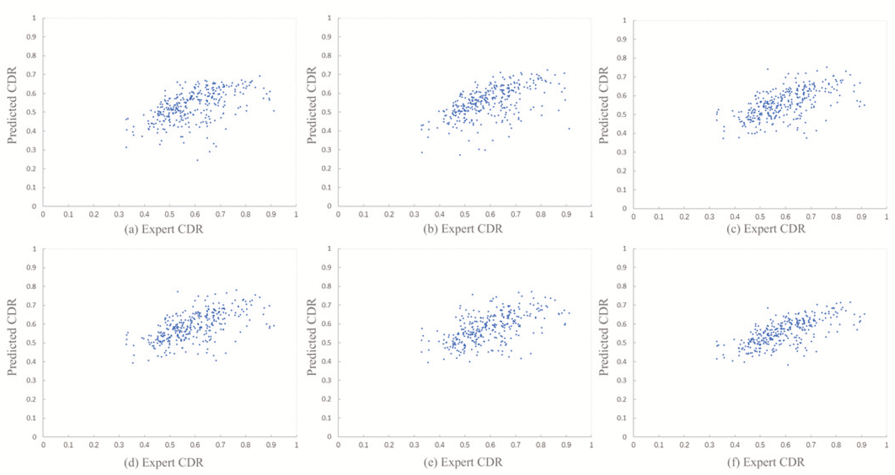
4.2.2. Pearson’s Correlation Coefficient

In order to measure the degree of correlation between predicted CDR and hand-labeled CDR, the statistical index of correlation coefficient is used and its definition is expressed as:

$$r=\frac{{\sum }_{i=1}^N(CD{R}_i^h-C\overline{D}{R}^h)(CD{R}_i^p-C\overline{D}{R}_p)}{\sqrt{{\sum }_{i=1}^N{(CD{R}^h-C\overline{D}{R}^h)}^2}\sqrt{{\sum }_{i=1}^N{(CD{R}_p-C\overline{D}{R}_p)}^2}}$$

(12)

where $CD{R}^h$s still are the experts CDR from the trained experts, and $CD{R}^p$s still is the CDR calculated after the segmentation masks of OD and OC is obtained.

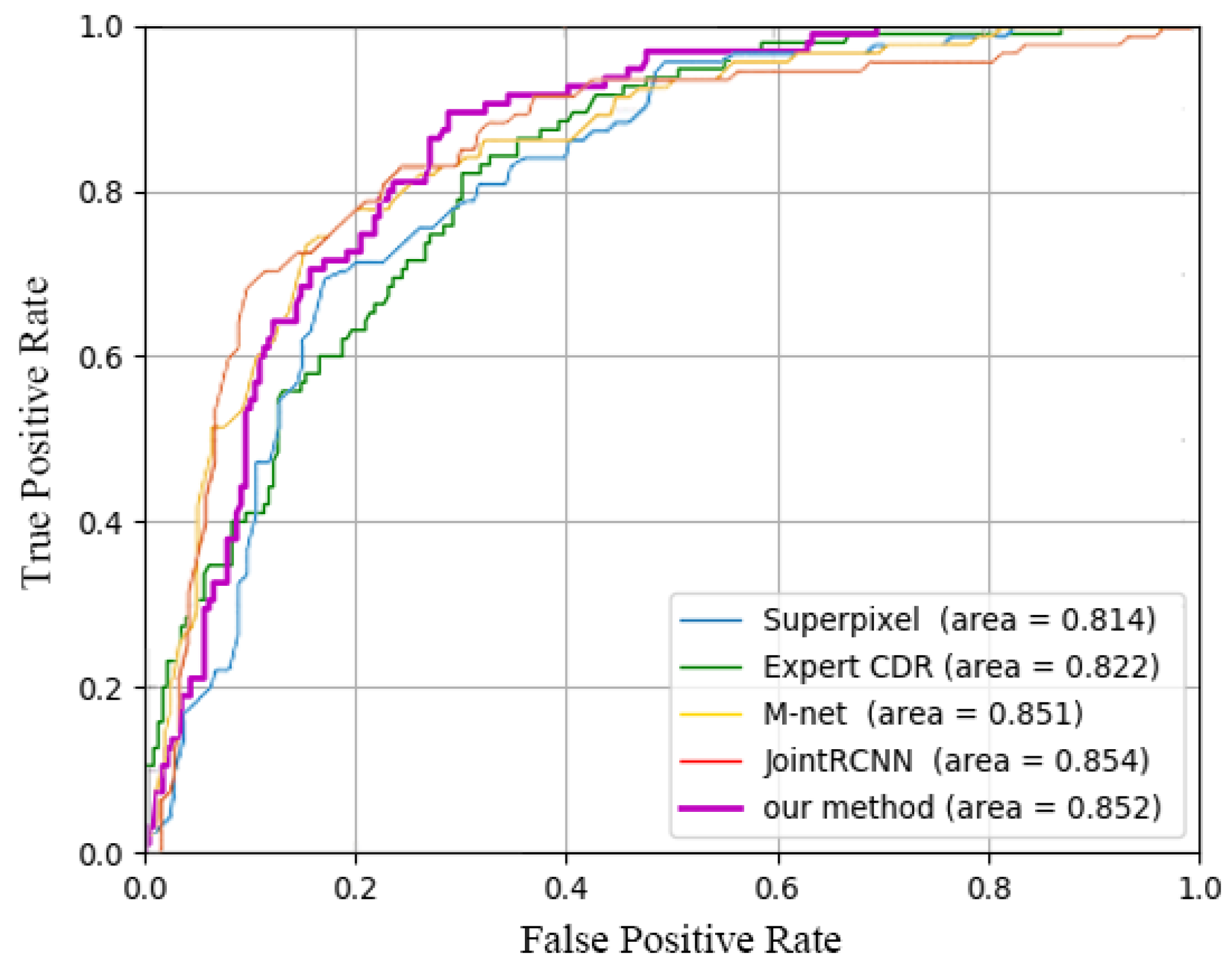
4.2.3. Screening for Glaucoma

We treat the obtained CDR as a probability number and calculate the receiver operating characteristic (ROC) curves and area under curve (AUC) to evaluate our method on glaucoma screening.

4.3. Performance Improvement with Two Attention Blocks

4.3.1. Ablation Study

For showing the effect of two attention blocks (SAB and CAB), we conduct the experiments of ablation study on the ORIGA dataset [49]. The result of different settings is shown in

Table 1. The results with and without channel attention block, spatial attention block and segmentation-auxiliary module.

Model	CAB	SAB	SAM	r	MAE	AUC
Baseline model	×	×	×	0.554	0.0823	0.806
	×	✓	×	0.580	0.0739	0.795
	✓	×	×	0.610	0.0728	0.830
	✓	✓	×	0.616	0.0698	0.831
	×	×	✓	0.586	0.0722	0.824
	✓	✓	✓	0.694	0.0671	0.852

.

Baseline model. Our baseline model is based on standard U-net, as the end of the model, we design a simple regression deep network to attain CDR number.

Baseline model + CAB. On the basis of 1, CAB is introduced.

Baseline model + SAB. Similarly, SAB is introduced by itself.

Baseline model + CAB + SAB. The full model consists of the U-net regression model, SAB and CAB.

Table 1 shows that both CAB and SAB achieve better performance. When the baseline model combines CAB, the MAE/AUC is 0.0728/0.830; when the baseline model combines SAB, the mean absolute error is 0.0739/0.795; When simultaneously adding SAB and CAB into the models, the proposed attains 0.0698/0.831 the best performance. Therefore, the combined learning of CAB and SAB can achieve excellent results.

The results of Pearson’s correlation coefficient are shown in Figure 5. As shown in Figure 5, with the addition of the two modules, the correlation between the predicted data and the data manually labeled by the doctor gradually increases.

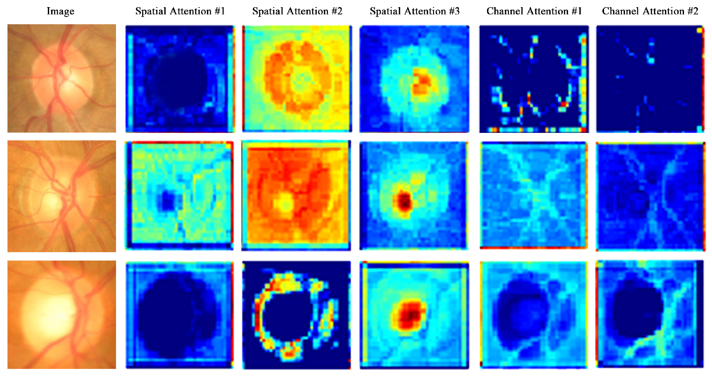
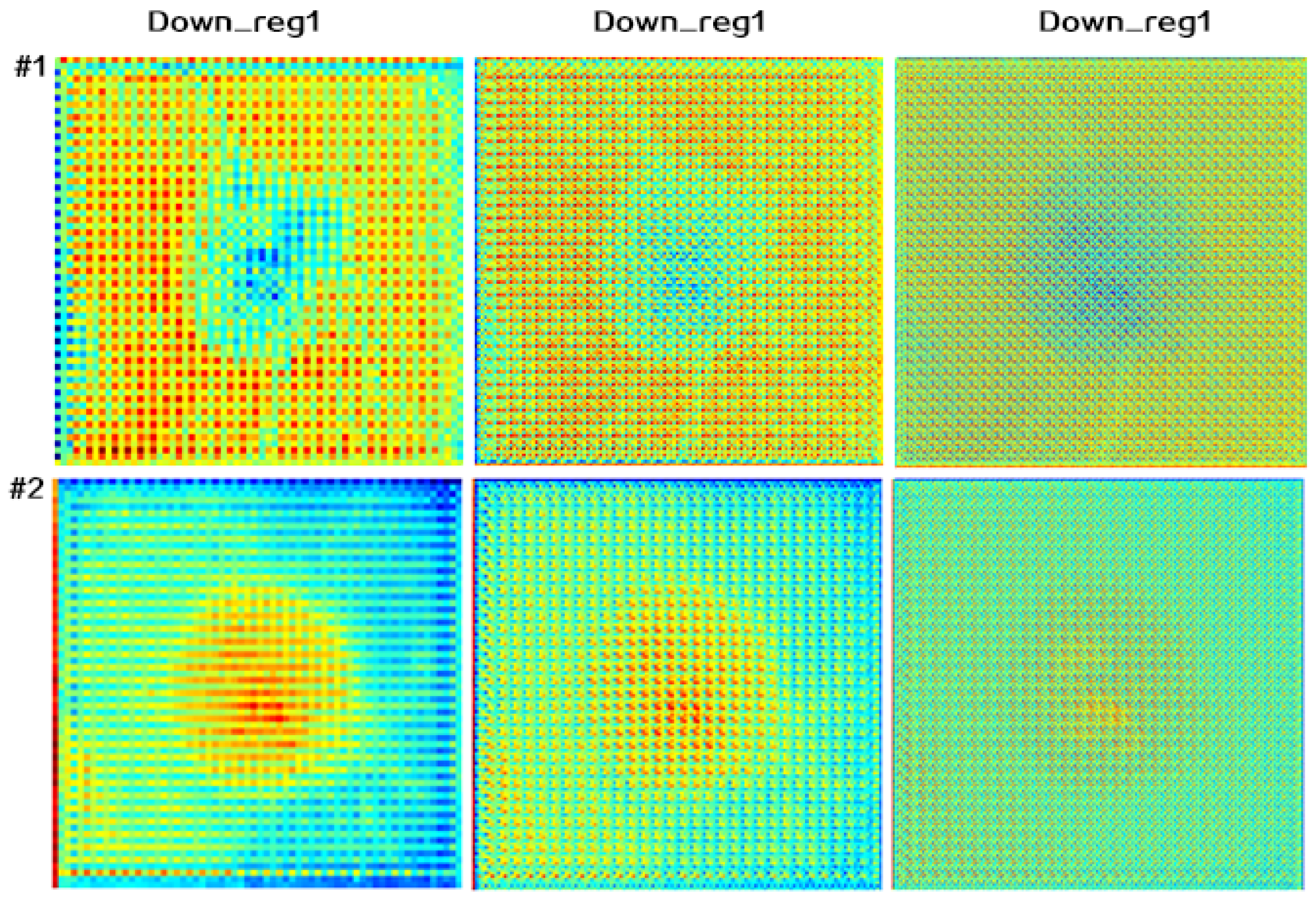
4.3.2. Attention Map Visualization

In proposed CSAR, CAB models in channel dimension which selects relatively important feature maps, shifting the emphasis on the OD and OC region; meanwhile, the SAB learns the discriminative ability of feature representation at pixel level by capturing the relationship of intra-feature map. What is remarkable about SAB is that it makes the classification of pixels on the boundary area more accurate. Here, we verify our conclusions by comparing visual feature maps. Figure 6 shows the visualization of attention maps, and we select maps #1–3 from all feature maps in two types of attention maps.

The experimental results show that the SAB can learn the discriminative ability of feature representation at the pixel level and capture the OD and OC area information. Map #1 does fine for the background area, map #2 is relatively sensitive to the rim area, and map #3 selectively segments the OC. For CAB, some features are selected to see whether it relatively suppresses semantic information with low responsiveness. For example, the response of vessel semantic information is relatively suppressive after CAB.

4.4. Benefit of Joint Learning Framework

4.4.1. Absolute CDR Error

In order to visually see that the auxiliary module is effective, we conduct an ablation study. The results are shown in Table 1.

In Table 1, the mean absolute error of the baseline model is 0.0823; when the baseline model combined with segmentation-auxiliary model, the mean absolute error is 0.0722. After the baseline model combines CAB, SAB and SAM, the final mean absolute error is 0.0671.

4.4.2. Attention Map Visualization

The segmentation-auxiliary can focus the model’s attention on the relevant features instead of the background region. In our experiments, the condition of map #1 is found which is shown in Figure 7, we could see the non-OD region is more responsive, to be specific, the CDR obtained by regression is from the background region, which is not what we want. To address this problem, the segmentation-auxiliary module is proposed due to the fact that the attention of OD and OC is easy to focus but it is difficult to learn via the single regression task.

4.5. Comparison with Exist Methods

We compare CSAR model with several start-of-art models, such as relevant-vessel bends (R-Bend) [25], active shape model (ASM) [48], Superpixel [29], Joint U-net + PT [12], M-net [12], JointRCNN [35]. The result is shown in

Table 2. The results of different methods.

Method	MAE	AUC	Coefficient
R-Bend [25]	0.154	-	0.38
ASM [48]	0.107	-	-
Superpixel [29]	0.077	0.814	0.59
Expert CDR estimation	0	0.823	-
Joint U-net + PT	0.075	0.8322	0.617
M-net [12]	0.071	0.8508	0.671
JointRCNN [35]	0.068	0.8536	-
Baseline+CAB+SAB	0.070	0.8310	0.616
Our method	0.067	0.8524	0.694

. It can be seen that the proposed model obtains the best MAE with similar result of AUC.

For the absolute CDR error, compared with the hand-craft methods, the deep learning methods are better. R-Bend [25] copes with the variations of OD regions by utilizing multidimensional feature space. ASM [48] takes advantage of the circular Hough to transform initialization to segment. The above two approaches do not obtain satisfactory performance. By contrast, Superpixel [29] addresses the OD and OC segmentation as a pixel classification task and obtains relatively satisfactory results. M-net [12], JointRCNN [35] obtain good results. In the paper, our proposed CSAR achieves a smaller error than those above. It demonstrates that the attention blocks and segmentation-auxiliary model are useful to guide the CDR calculation.

For the AUC results, the following conclusions are reached: (1) The non-deep learning method called Superpixel [29] surprisingly achieves excellent performance in screening glaucoma. (2) Compared with the traditional methods, the current methods combining deep leaning such as M-net [12], JointRCNN [35] successively increase. (3) In particular, experimental results in the screening of glaucoma is similar to the other two proposed deep learning methods. Our model reduces the CDR error rate while ensuring that the AUC is similar. The ROC curves of different methods are shown in Figure 8.

For the Pearson’s correlation coefficient, compared with R-Bend [25] (0.38), Superpixel [29] obtains relatively satisfactory results (0.59). Joint U-net and M-net also obtain good results (0.617, 0.671). In the paper, our proposed CSAR achieves better results than those above. It demonstrates that jointly leaning of attention blocks and regression network is useful to predict the CDR number.

In our experiment, we also use the T-test to compare our method with other methods. The test results (p-value, t) reveal the difference between the existing method (<0.01, 5.506) and the proposed method, such as R-bend (<0.01, 3.077), Superpixel (<0.01, 4.021), and M-net (<0.01, 4.948).

In our testing, our method costs only 0.06s to regress the final CDR number for one fundus image on NVIDIA Tesla GPU. This is faster than most existing methods, such as R-Bend (4 s), ASM (4s), Superpixel (10 s), and M-net (0.5 s).

4.6. Discuss

In addition to the CDR, ISNT rule is utilized for screening for glaucoma [50]. The ISNT rule is the ordering of rim area of inferior, superior, nasal and temporal regions in order as:

$$I\succ S\succ N\succ T$$

(13)

where I represents inferior regions, S represents superior regions, N represents nasal regions, and T represents temporal regions. The samples which follow this rule are considered as healthy while others are suspected as glaucomatous. These four area markers are shown in Figure 9.

In our experiment, We replace the network that returns CDR number with a regression network that simultaneously returns the four numbers ISNT. Then, samples meeting the above rules will be considered normal, otherwise glaucoma. We can find that the rim error is more significant than the ratio error. The AUC calculated by ISNT is 0.587, which is lower than CDR measurement but higher than ISNT that obtained from the labels manually marked by ophthalmologists (0.540). The main reason, presumably, lies in the fact that the measurement method of ISNT has a lot to do with their position, and the attention of regression mapping is challenging to be accurate. Simultaneously compared with the AUC computed by experts CDR values, the AUC computed by ISNT that obtained from the labels manually marked by ophthalmologists is relatively low, maybe because it reacts poorly to non-glaucomatous large optic cups samples.

Complexity analysis plays an important role in measuring the efficiency of an algorithm. We calculate the number of parameters and the FLOPs to evaluate our algorithm. In our experiment, compared with the standard U-net, our model makes the number of parameters and the FLOPs increase to a certain extent. In future, self-attention mechanism can be further created for capturing global information, and the GPU memory friendly and High computational efficiency can be an excellent sign to guide the future research work.

5. Conclusions

A multitask deep network is proposed to directly regress CDR number and simultaneously combine two attention blocks called SAB and CAB. It is the first time that the regression network combines the self-attention mechanism and is used for screening for glaucoma. Auxiliary leaning of segmentation is first employed in CDR estimation. Experimental results show that more accurate numbers can be produced by our CSAR model. Thus, we believe that the proposed attention blocks are easily applied to other tasks because of its simplicity and lightness, such as image segmentation, image registration and so on. In future studies, this is what will be tested.

References

1. Almazroa, A.; Burman, R.; Raahemifar, K.; Lakshminarayanan, V. Optic disc and optic cup segmentation methodologies for glaucoma image detection: A survey. J. Ophthalmol. 2015, 2015, 180972. [Google Scholar] [CrossRef] [PubMed] [Green Version]
2. Hagiwara, Y.; Koh, J.E.W.; Tan, J.H.; Bhandary, S.V.; Laude, A.; Ciaccio, E.J.; Tong, L.; Acharya, U.R. Computer-aided diagnosis of glaucoma using fundus images: A review. Comput. Methods Programs Biomed. 2018, 165, 1–12. [Google Scholar] [CrossRef] [PubMed]
3. Pathan, S.; Kumar, P.; Pai, R.M. Segmentation Techniques for Computer-Aided Diagnosis of Glaucoma: A Review. In Advances in Machine Learning and Data Science (NIPS); Springer: Singapore, 2018; pp. 163–173. [Google Scholar]
4. Lian, J.; Hou, S.; Sui, X.; Xu, F.; Zheng, Y. Deblurring retinal optical coherence tomography via a convolutional neural network with anisotropic and double convolution layer. Comput. Vis. IET 2018, 12, 900–907. [Google Scholar] [CrossRef]
5. Thakur, N.; Juneja, M. Survey on segmentation and classification approaches of optic cup and optic disc for diagnosis of glaucoma. Biomed. Signal Process. Control 2018, 42, 162–189. [Google Scholar] [CrossRef]
6. Fumero, F.; Sigut, J.; Alayón, S.; González-Hernández, M.; González de la Rosa, M. Interactive Tool and Database for Optic Disc and Cup Segmentation of Stereo and Monocular Retinal Fundus Images; Vaclav Skala-UNION Agency: Plzen, Czech Republic, 2015. [Google Scholar]
7. Guo, J.; Azzopardi, G.; Shi, C.; Jansonius, N.M.; Petkov, N. Automatic determination of vertical cup-to-disc ratio in retinal fundus images for glaucoma screening. IEEE Access 2019, 7, 8527–8541. [Google Scholar] [CrossRef]
8. Wang, Q.; Zheng, Y.; Yang, G.; Jin, W.; Chen, X.; Yin, Y. Multi-Scale Rotation-Invariant Convolutional Neural Networks for Lung Texture Classification. IEEE J. Biomed. Health Inform. 2017, 21, 184–195. [Google Scholar]
9. Liang, D.; Yang, F.; Wang, X.; Ju, X. Multi-Sample Inference Network. IET Comput. Vis. 2019, 36, 605–613. [Google Scholar] [CrossRef]
10. Long, J.; Shelhamer, E.; Darrell, T. Fully convolutional networks for semantic segmentation. In Proceedings of the IEEE Conference on Computer Vision and Pattern Recognition, Boston, MA, USA, 7–12 June 2015; pp. 3431–3440. [Google Scholar]
11. Ronneberger, O.; Fischer, P.; Brox, T. U-net: Convolutional networks for biomedical image segmentation. In Proceedings of the International Conference on Medical Image Computing and Computer-Assisted Intervention (MICCAI), Munich, Germany, 5–9 October 2015; pp. 234–241. [Google Scholar]
12. Fu, H.; Cheng, J.; Xu, Y.; Wong, D.W.K.; Liu, J.; Cao, X. Joint optic disc and cup segmentation based on multi-label deep network and polar transformation. IEEE Trans. Med. Imaging 2018, 37, 1597–1605. [Google Scholar] [CrossRef] [Green Version]
13. Mary, V.S.; Rajsingh, E.B.; Naik, G.R. Retinal fundus image analysis for diagnosis of glaucoma: A comprehensive survey. IEEE Access 2016, 4, 4327–4354. [Google Scholar] [CrossRef]
14. Zheng, Y.; Zhang, S.; Huang, J.; Cai, W. Guest Editorial: Special issue on advances in computing techniques for big medical image data. Neurocomputing 2016, 100, S0925231216313704. [Google Scholar] [CrossRef]
15. Sui, X.; Zheng, Y.; Wei, B.; Bi, H.; Wu, J.; Pan, X.; Yin, Y.; Zhang, S. Choroid segmentation from Optical Coherence Tomography with graph edge weights learned from deep convolutional neural networks. Neurocomputing 2017, 237, 332–341. [Google Scholar] [CrossRef]
16. Hou, S.; Zhou, S.; Liu, W.; Zheng, Y. Classifying advertising video by topicalizing high-level semantic concepts. Multimed. Tools Appl. 2018, 77, 25475–25511. [Google Scholar] [CrossRef]
17. Jiang, Y.; Zheng, Y.; Hou, S.; Chang, Y.; James, G. Multimodal Image Alignment via Linear Mapping between Feature Modalities. J. Healthc. Eng. 2017, 2017, 8625951. [Google Scholar] [CrossRef] [Green Version]
18. Deng, X.; Zheng, Y.; Xu, Y.; Xi, X.; Li, N.; Yin, Y. Graph cut based automatic aorta segmentation with an adaptive smoothness constraint in 3D abdominal CT images. Neurocomputing 2018, 310, 46–58. [Google Scholar] [CrossRef]
19. Khalil, T.; Akram, M.U.; Raja, H.; Jameel, A.; Basit, I. Detection of glaucoma using cup to disc ratio from spectral domain optical coherence tomography images. IEEE Access 2018, 6, 4560–4576. [Google Scholar] [CrossRef]
20. Lee, K.; Niemeijer, M.; Garvin, M.K.; Kwon, Y.H.; Sonka, M.; Abramoff, M.D. Segmentation of the optic disc in 3-D OCT scans of the optic nerve head. IEEE Trans. Med. Imaging 2009, 29, 159–168. [Google Scholar]
21. Wu, M.; Leng, T.; de Sisternes, L.; Rubin, D.L.; Chen, Q. Automated segmentation of optic disc in SD-OCT images and cup-to-disc ratios quantification by patch searching-based neural canal opening detection. Opt. Express. 2015, 23, 31216–31229. [Google Scholar] [CrossRef] [PubMed]
22. Fu, H.; Xu, D.; Lin, S.; Wong, D.W.K.; Liu, J. Automatic optic disc detection in oct slices via low-rank reconstruction. IEEE Trans. Biomed. Eng. 2014, 62, 1151–1158. [Google Scholar] [CrossRef]
23. Fu, H.; Xu, Y.; Lin, S.; Zhang, X.; Wong, D.W.K.; Liu, J.; Frangi, A.F.; Baskaran, M.; Aung, T. Segmentation and quantification for angle-closure glaucoma assessment in anterior segment OCT. IEEE Trans. Med. Imaging 2017, 36, 1930–1938. [Google Scholar] [CrossRef] [Green Version]
24. Lowell, J.; Hunter, A.; Steel, D.; Basu, A.; Ryder, R.; Fletcher, E.; Kennedy, L. Optic nerve head segmentation. IEEE Trans. Med. Imaging 2004, 23, 256–264. [Google Scholar] [CrossRef] [Green Version]
25. Joshi, G.D.; Sivaswamy, J.; Krishnadas, S. Optic disk and cup segmentation from monocular color retinal images for glaucoma assessment. IEEE Trans. Med. Imaging 2011, 30, 1192–1205. [Google Scholar] [CrossRef] [PubMed]
26. Abramoff, M.D.; Alward, W.L.; Greenlee, E.C.; Shuba, L.; Kim, C.Y.; Fingert, J.H.; Kwon, Y.H. Automated segmentation of the optic disc from stereo color photographs using physiologically plausible features. Investig. Ophthalmol. Vis. Sci. 2007, 48, 1665–1673. [Google Scholar] [CrossRef] [PubMed]
27. Zahoor, M.N.; Fraz, M.M. Fast optic disc segmentation in retina using polar transform. IEEE Access 2017, 5, 12293–12300. [Google Scholar]
28. Zheng, Y.; Stambolian, D.; O’Brien, J.; Gee, J.C. Optic disc and cup segmentation from color fundus photograph using graph cut with priors. In Proceedings of the International Conference on Medical Image Computing and Computer-Assisted Intervention, Nagoya, Japan, 22–26 September 2013; pp. 75–82. [Google Scholar]
29. Cheng, J.; Liu, J.; Xu, Y.; Yin, F.; Wong, D.W.K.; Tan, N.M.; Tao, D.; Cheng, C.Y.; Aung, T.; Wong, T.Y. Superpixel classification based optic disc and optic cup segmentation for glaucoma screening. IEEE Trans. Med. Imaging 2013, 32, 1019–1032. [Google Scholar] [CrossRef] [PubMed]
30. Sevastopolsky, A. Optic disc and cup segmentation methods for glaucoma detection with modification of U-Net convolutional neural network. Pattern Recognit. Image Anal. 2017, 27, 618–624. [Google Scholar] [CrossRef] [Green Version]
31. Qin, Y.; Hawbani, A. A Novel Segmentation Method for Optic Disc and Optic Cup Based on Deformable U-net. In Proceedings of the International Conference on Artificial Intelligence and Big Data, ICAIBD, Chengdu, China, 25–28 May 2019; pp. 394–399. [Google Scholar]
32. Shankaranarayana, S.M.; Ram, K.; Mitra, K.; Sivaprakasam, M. Joint optic disc and cup segmentation using fully convolutional and adversarial networks. In Fetal, Infant and Ophthalmic Medical Image Analysis; Springer: Cham, Switzerland, 2017; pp. 168–176. [Google Scholar]
33. Wang, S.; Yu, L.; Yang, X.; Fu, C.W.; Heng, P.A. Patch-based output space adversarial learning for joint optic disc and cup segmentation. IEEE Trans. Med. Imaging 2019, 38, 2485–2495. [Google Scholar] [CrossRef] [Green Version]
34. Jiang, Y.; Tan, N.; Peng, T. Optic Disc and Cup Segmentation Based on Deep Convolutional Generative Adversarial Networks. IEEE Access 2019, 7, 64483–64493. [Google Scholar]
35. Jiang, Y.; Duan, L.; Cheng, J.; Gu, Z.; Xia, H.; Fu, H.; Li, C.; Liu, J. JointRCNN: A Region-based Convolutional Neural Network for Optic Disc and Cup Segmentation. IEEE Trans. Biomed. Eng. 2019, 67, 335–343. [Google Scholar]
36. Zhao, R.; Chen, X.; Xiyao, L.; Zailiang, C.; Guo, F.; Li, S. Direct cup-to-disc ratio estimation for glaucoma screening via semi-supervised learning. IEEE J. Biomed. Health Inform. 2019, 24, 1104–1113. [Google Scholar] [CrossRef]
37. Mnih, V.; Heess, N.; Graves, A. Recurrent models of visual attention. In Proceedings of the Advances in Neural Information Processing Systems, Montreal, QC, Canada, 8–13 December 2014; pp. 2204–2212. [Google Scholar]
38. Sutskever, I.; Vinyals, O.; Le, Q.V. Sequence to sequence learning with neural networks. In Proceedings of the Advances in Neural Information Processing Systems, Montreal, QC, Canada, 8–13 December 2014; pp. 3104–3112. [Google Scholar]
39. Lu, X.; Chen, Y.; Li, X. Hierarchical recurrent neural hashing for image retrieval with hierarchical convolutional features. IEEE Trans. Image Process. 2017, 27, 106–120. [Google Scholar]
40. Xu, K.; Ba, J.; Kiros, R.; Cho, K.; Courville, A.; Salakhudinov, R.; Zemel, R.; Bengio, Y. Show, attend and tell: Neural image caption generation with visual attention. In Proceedings of the International Conference on Machine Learning, Lille, France, 6–11 July 2015; pp. 2048–2057. [Google Scholar]
41. Vaswani, A.; Shazeer, N.; Parmar, N.; Uszkoreit, J.; Jones, L.; Gomez, A.N.; Kaiser, Ł.; Polosukhin, I. Attention is all you need. In Proceedings of the Advances in Neural Information Processing Systems, Long Beach, CA, USA, 4–9 December 2017; pp. 5998–6008. [Google Scholar]
42. Wang, X.; Girshick, R.; Gupta, A.; He, K. Non-local neural networks. In Proceedings of the IEEE Conference on Computer Vision and Pattern Recognition, Salt Lake City, UT, USA, 18–22 June 2018; pp. 7794–7803. [Google Scholar]
43. Du, Y.; Yuan, C.; Li, B.; Zhao, L.; Li, Y.; Hu, W. Interaction-aware spatio-temporal pyramid attention networks for action classification. In Proceedings of the European Conference on Computer Vision, Munich, Germany, 4–8 September 2018; pp. 373–389. [Google Scholar]
44. Woo, S.; Park, J.; Lee, J.Y.; So Kweon, I. Cbam: Convolutional block attention module. In Proceedings of the European Conference on Computer Vision, Munich, Germany, 4–8 September 2018; pp. 3–19. [Google Scholar]
45. Li, L.; Xu, M.; Wang, X.; Jiang, L.; Liu, H. Attention based glaucoma detection: A large-scale database and CNN Model. In Proceedings of the IEEE Conference on Computer Vision and Pattern Recognition, Long Beach, CA, USA, 16–20 June 2019; pp. 10571–10580. [Google Scholar]
46. Fu, J.; Liu, J.; Tian, H.; Li, Y.; Bao, Y.; Fang, Z.; Lu, H. Dual attention network for scene segmentation. In Proceedings of the IEEE Conference on Computer Vision and Pattern Recognition, Long Beach, CA, USA, 16–20 June 2019; pp. 3146–3154. [Google Scholar]
47. Kendall, A.; Gal, Y.; Cipolla, R. Multi-task learning using uncertainty to weigh losses for scene geometry and semantics. In Proceedings of the IEEE Conference on Computer Vision and Pattern Recognition, Salt Lake City, UT, USA, 18–22 June 2018; pp. 7482–7491. [Google Scholar]
48. Yin, F.; Liu, J.; Ong, S.H.; Sun, Y.; Wong, D.W.; Tan, N.M.; Cheung, C.; Baskaran, M.; Aung, T.; Wong, T.Y. Model-based optic nerve head segmentation on retinal fundus images. In Proceedings of the Annual International Conference of the IEEE Engineering in Medicine and Biology, Boston, MA, USA, 30 August–3 September 2011; pp. 2626–2629. [Google Scholar]
49. Zhang, Z.; Yin, F.S.; Liu, J.; Wong, W.K.; Tan, N.M.; Lee, B.H.; Cheng, J.; Wong, T.Y. Origa-light: An online retinal fundus image database for glaucoma analysis and research. In Proceedings of the nnual International Conference of the IEEE Engineering in Medicine and Biology, Buenos Aires, Argentina, 31 August–4 September 2010; pp. 3065–3068. [Google Scholar]
50. Harizman, N.; Oliveira, C.; Chiang, A.; Tello, C.; Marmor, M.; Ritch, R.; Liebmann, J.M. The ISNT rule and differentiation of normal from glaucomatous eyes. Arch. Ophthalmol. 2006, 124, 1579–1583. [Google Scholar] [CrossRef] [PubMed] [Green Version]
Figure 1. Overview of Channel and Spatial Attention Regression Network, which combines a deep convolution neural network (CNN) for cropping optic disc and optic cup areas, the encode, two parallel attention modules called channel attention block (CAB) and spatial attention block (SAB), the decode, and a multitask relationship learning module for cup-to-disc ratio number estimation. Here, the “conv” is denoted as convolutional layer, the “down_rep” represents three down-sampling layers and the “conv-64” means convolution layer with kernel size 64 × 64.
Electronics 09 00909 g001
Figure 2. The detailed architectures of the spatial attention block in CSAR.
Electronics 09 00909 g002
Figure 3. The detailed architectures of the channel attention block in CSAR.
Electronics 09 00909 g003
Figure 4. The segmentation-auxiliary task is introduced into our model which is parallel to the main regression task. During the test, our model works in an implicit way for which image segmentation information is considered but not displayed.
Electronics 09 00909 g004
Figure 5. Comparison of Pearson’s correlation coefficient of different methods. (a) Baseline model. (b) Baseline model + SAB. (c) Baseline model + CAB. (d) Baseline model + CAB + SAB. (e) Baseline model + SAM. (f) Baseline model + CAB + SAB + SAM.
Electronics 09 00909 g005
Figure 6. Examples of the two attention blocks. Column 1: input image, Column 2, 3 and 4: the maps of spatial attention block, Column 4 and 5: the maps of channel attention block.
Electronics 09 00909 g006
Figure 7. Examples of special circumstances. First row: the CDR obtained by regression is from the background region, second row: the CDR obtained by regression is from the OD and OC region. Here the “down_reg i” represents the ith down-sampling layer.
Electronics 09 00909 g007
Figure 8. Comparison of ROC curves of different methods.
Electronics 09 00909 g008
Figure 9. (a) The fundus image. (b) The green area represents the optic cup and the golden area denotes the optic disc. Here an example of ISNT rules is shown. (c) An example of CDR calculation is presented.
Electronics 09 00909 g009