EANN: Energy Adaptive Neural Networks

Abstract

This paper proposes an Energy Adaptive Feedforward Neural Network (EANN). It uses multiple approximation techniques in the hardware implementation of the neuron unit. The used techniques are precision scaling, approximate multiplier, computation skipping, neuron skipping, activation function approximation and truncated accumulation. The proposed EANN system applies the partial dynamic reconfiguration (PDR) feature supported by the FPGA platform to reconfigure the hardware elements of the neural network based on the energy budget. The PDR technique enables the EANN system to remain functioning when the available energy budget is reduced by factors of 46.2% to 79.8% of the total energy of the unapproximated neural network. Unlike the conventional operation that only uses certain amount of energy and cannot function properly if the energy budget falls below that energy level, the EANN system remains functioning for longer time after energy drop at the expense of less accuracy. The proposed EANN system is highly recommended in limited-energy applications as it adapts the hardware units to the degraded energy at the expense of some accuracy loss.

1. Introduction

Artificial Neural Networks (ANNs) are brain inspired systems that can be used in a wide range of applications that need intensive and complex processing. Neural networks are used in various applications such as classification, pattern recognition, data analysis and computer vision [1]. The neural networks are superior over the traditional algorithms due to the learning capabilities and the availability of large data sets.

Feedforward neural network is the commonly used ANN. The ANN basic structure consists of input layer, one or more hidden layers, and output layer as shown in Figure 1. In each layer, the basic processing element is the neuron in which the weights are multiplied by the inputs and then the multiplication results are added using accumulators. Following that, the output of the accumulators is passed through an activation function that adds some non-linearity to the output product to mimic the human brain processes. The output of each layer is the input to the next layer till the output layer is reached. The weights associated with each input are adjusted during the training phase (offline training) to get the maximum possible accuracy of the network.

Hardware implementation of ANN requires intensive computations as it uses many processing elements (neurons). Each processing element has many arithmetic operations such as multiplications, accumulations and activation function which consume area and power, especially the multiplication operations. As the number of network layers or the number of neurons in each layer increase, the power and the area of the hardware system are increased. Hardware implementation of such networks has several challenges which are studied from different perspectives in [2]. The fact that ANNs are used in error resilience applications has permitted some approximation in the hardware implementation of them. Research work has been carried out to achieve energy-efficient hardware implementation for the ANNs. Approximate computing has been studied from different perspectives in [3,4,5,6,7,8].

There is a variety of ANN approximation techniques to save area and power which are the main concern in the hardware systems, especially, low power applications. These approximations degrade the accuracy of the ANN. Fortunately, ANNs are used in error resilience applications and accordingly, 100% accuracy is not mandatory. As a result, the hardware implementation should have low area and power consumption at the expense of accuracy degradation. The target of the approximate computing is to have the optimal power and area trade-offs with minimum degradation in accuracy. The most common approximation techniques are:

• Precision scaling: the data is represented as fixed-point numbers and the word length is reduced to reduce the number of bits per word. Correspondingly, the sizes of multiplier, accumulators, and activation function are reduced and the area, power, and accuracy are reduced as well.
• Inaccurate arithmetic: As the neural network uses many multipliers and adders which are power-hungry hardware units. These units should be implemented in approximate versions to save power and area.
• Neuron skipping(pruning): It is another approximation technique in which the neurons that have the least contribution in the outputs are skipped from the computation or at least they are implemented with approximation. This reduces the number of cycles needed to perform the operations and reduces the total required energy as well.
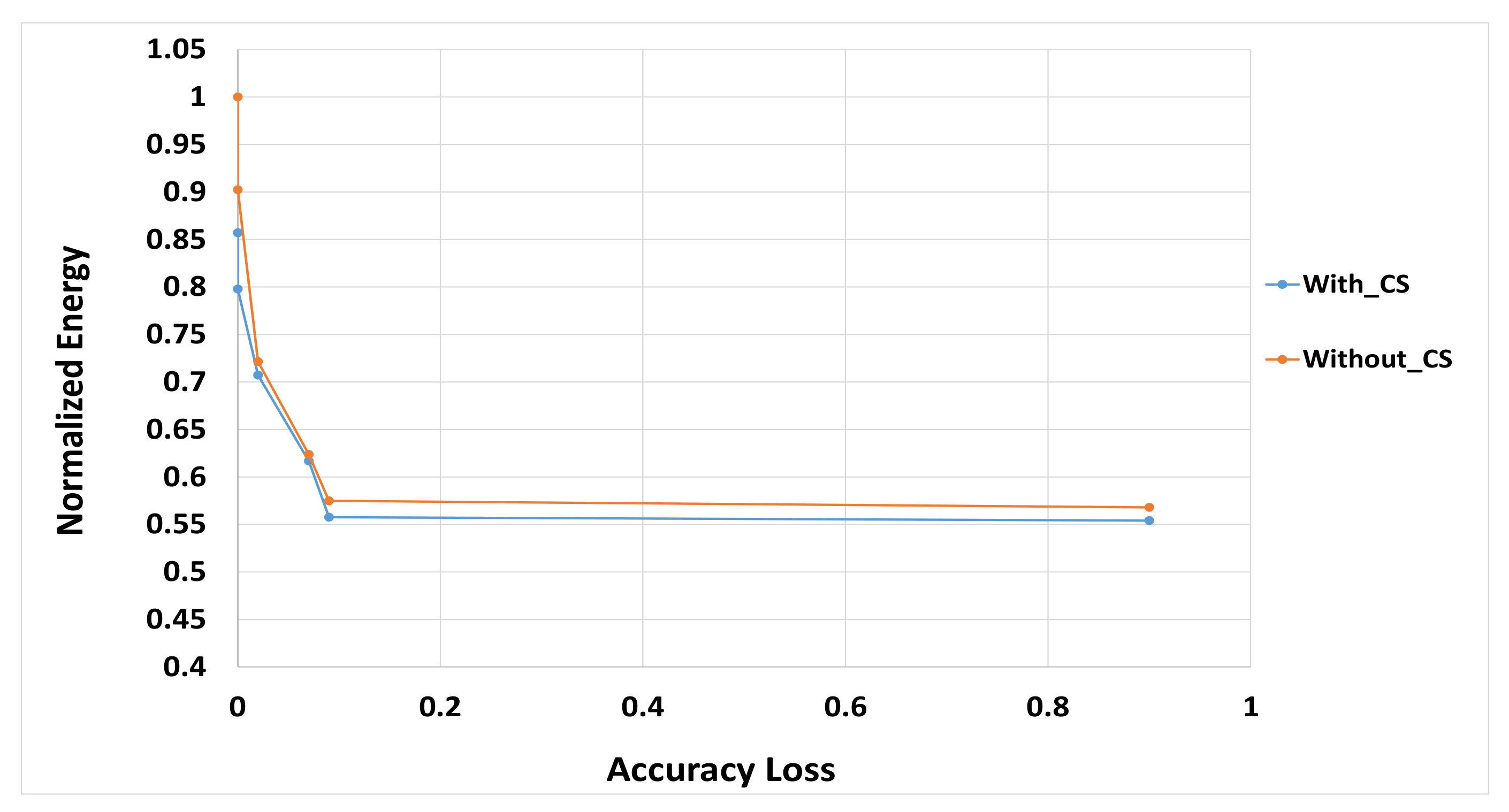
• Computation skipping: The input data might contain lots of zeros which do not affect the result after multiplication or addition. Thus, there is a hardware unit that checks the input value and bypasses the upcoming computations if this input value equals zero. This lowers the activity factor and saves much dynamic power. This technique is valuable only in the case when the input contains many zeros. Otherwise, it would consume area and power for the zero-detection hardware unit without decreasing the dynamic power.
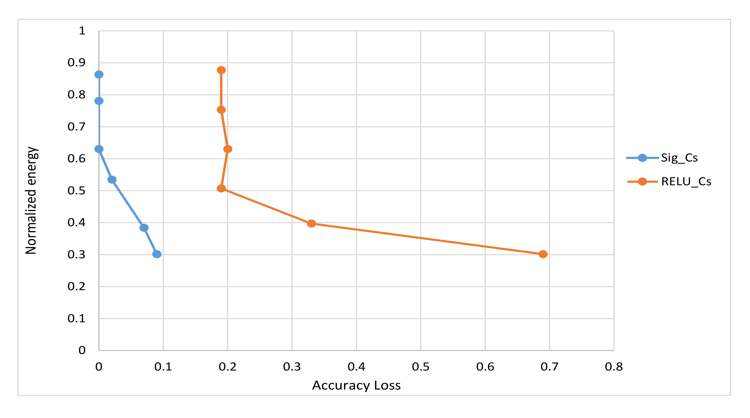
• Approximate activation function: The commonly used activation function is Sigmoid which contains exponential in its formula. If it is implemented in an exact way it consumes large area and power. Therefore, the approximated version of the Sigmoid function such as Piece-Wise Linear (PWL) approximation helps in saving power and area with degradation in accuracy.

In this paper, the previous approximation techniques on the ANN are adopted to design an energy adaptive neural network (EANN) that reconfigures the neural network hardware units with the suitable approximations to meet the available energy budget of the application. This energy adaptation comes at the expense of lower accuracy. In this work, an energy adaptive neural network is introduced which adapts its hardware units according to a given available energy budget. In the non-adaptive systems, if the available energy is not sufficient for the hardware unit to operate, the hardware units stop functioning. Given the power profile of the system with time, the EANN system can predict the available energy and thus, if the energy is not sufficient the hardware is reconfigured and adapted to work with this lower available energy at the expense of accuracy degradation.

The reconfiguration technique used in this work is denoted by Partial Dynamic Reconfiguration (PDR). The idea of hardware reconfiguration is first introduced in [9]. In [9], it has been shown that a part of the hardware system could be static and controls the other part which is reconfigurable or dynamic to perform a specific task at a specific scheduled time. Since FPGAs are programmable, they could be used efficiently as a hardware reconfigurable platform. In the PDR, the hardware modules are dynamically changed within an active design in response to the available application energy requirements. The reconfiguration task is conducted in the run-time with no need to switch OFF the system for reconfiguration. The PDR technique is highly recommended when the application has multiple configurations to choose among and to reuse the same hardware physical resources for all configurations instead of implementing each configuration separately. For example, PDR technique has been adopted efficiently to reconfigure the communication chains according to the required wireless standards in software defined radio applications in [10]. The advantages of using the PDR technique is the flexibility of redefining the modules according to the dynamic requirements. It also saves much area since there is no need to implement all different configurations of the design, and build a controller to switch between these different configurations, instead they are reconfigured and replaced.

As an example for the low power applications that benefits from the PDR technique is the low-cost battery-powered wireless image sensor of precision agriculture. This application is used to perform pest control monitoring and is based on the use of insect traps conveniently spread over the specified control area. Depending on the targeted insect, each trap is properly installed with pheromones or other chemical substances that attract the insect that is intended to be captured. The wireless image sensor function is to classify the number of insects around the trap. When the battery energy is low, the neural network that performs the classification task reconfigures itself to a lower classification accuracy. As a result, the battery life lasts for more time.

The rest of the paper is organized as follows: Section 2 presents the related work previously published in the literature; Section 3 presents approximate computing techniques in detail and the proposed algorithm; Section 4 presents the simulation and experimental results on the neuron unit and on the overall proposed EANN system; Section 4 shows the Partial Dynamic Reconfiguration technique and Section 5 concludes the paper.

2. Related Work

Approximate computing is popular in the hardware implementation of artificial neural networks to achieve energy-efficient systems. A survey of techniques for approximate computing is provided in [11].

Venkataramani et al. [3] have proposed an approximation method based on identifying the error-resilient neurons that have the least effect on the output by using the backpropagation algorithm. Following that, the identified neurons have been replaced them by an approximated version that is more energy-efficient. They have used precision scaling in which the precision of inputs and weights of neurons is adapted based on their effect on the output. They also have used the Piece-Wise Linear (PWL) approximation of the Sigmoid function. After approximation, retraining is performed to enhance the output of the network and compensate for the approximation. They also have designed a quality-configurable Neuromorphic Processing Engine (qcNPE), which provides a programmable hardware platform for efficiently executing Approximate Artificial Neural Networks (AxNNs) with arbitrary topologies, weights, and degrees of approximation.

Zhang et al. [4] have proposed another method for identifying the error-resilient neurons. If a small jitter in the neuron computation has caused a large degradation in the output quality, then the neuron is critical and cannot be approximated. On the other hand, if the neuron is error-resilient, it can be approximated. After identifying the criticality of each neuron, an algorithm has been applied to rank and approximate the neurons. In [4], three approximation techniques are used namely: memory access skipping (if the neuron is considered uncritical, then skip reading the weights from memory and this saves the energy of memory access), approximate arithmetic (the use of approximate multipliers which are the most power-hungry hardware components) and precision scaling.

Kung et al. [5] have identified the neurons that have the least impact on the output using the greedy algorithm and the error sensitivity has been calculated during the training phase. The selected neurons have been implemented with reduced bit-precision and/or approximate multipliers proposed in [12,13]. The system has been designed in 130nm CMOS technology and an external DRAM is used as a memory interface.

Sarwar et al. [6] have proposed Alphabet Set Multiplier (ASM) in which the conventional multiplication has been replaced by shift and add operations. The product has been generated from smaller bit sequences, which are the lower order multiples of the multiplier input (alphabets). ASM contains a pre-computer bank that generates some alphabets. According to this approximation, all multiplication combinations are not supported and accordingly, the weights should be adjusted in the training phase.

Mrazek et al. [7] have proposed a methodology for the design of power-efficient neural network that has a uniform structure (all nodes are identical in all layers). The initial network design has no approximation adopted. Following that, several approximations have been adopted using an algorithm that identifies the approximation error. Several error metrics have been used by the proposed algorithm in [7] such as the average error magnitude and the maximum arithmetic error.

Kim et al. [8] have proposed a network that is designed for on-chip training. This on-chip training has been adopted by studying the effectiveness of the network design parameters such as the number of training iterations and the number of MLP (Multilayer perceptron) layers on the approximation techniques and the power consumption savings. The approximation techniques used in [8] are bit-precision scaling and approximate multiplier.

In summary, many research works have been proposed for the hardware implementation of ANN. The most common approximation methods are precision scaling, approximate arithmetic, computation skipping, activation function approximation and neuron skipping. All the work has been directed on how to find the best combination of these approximation methods.

3. Research Hypothesis, Design Approach and Methodology

This work considers most of the well-known power-efficient approximation techniques in designing an energy adaptive neural network. It is also the first paper to use the partial dynamic reconfiguration feature of the FPGA to implement the energy adaptive neural networks in such a way to compromise between the available energy budget and the highest possible accuracy results.

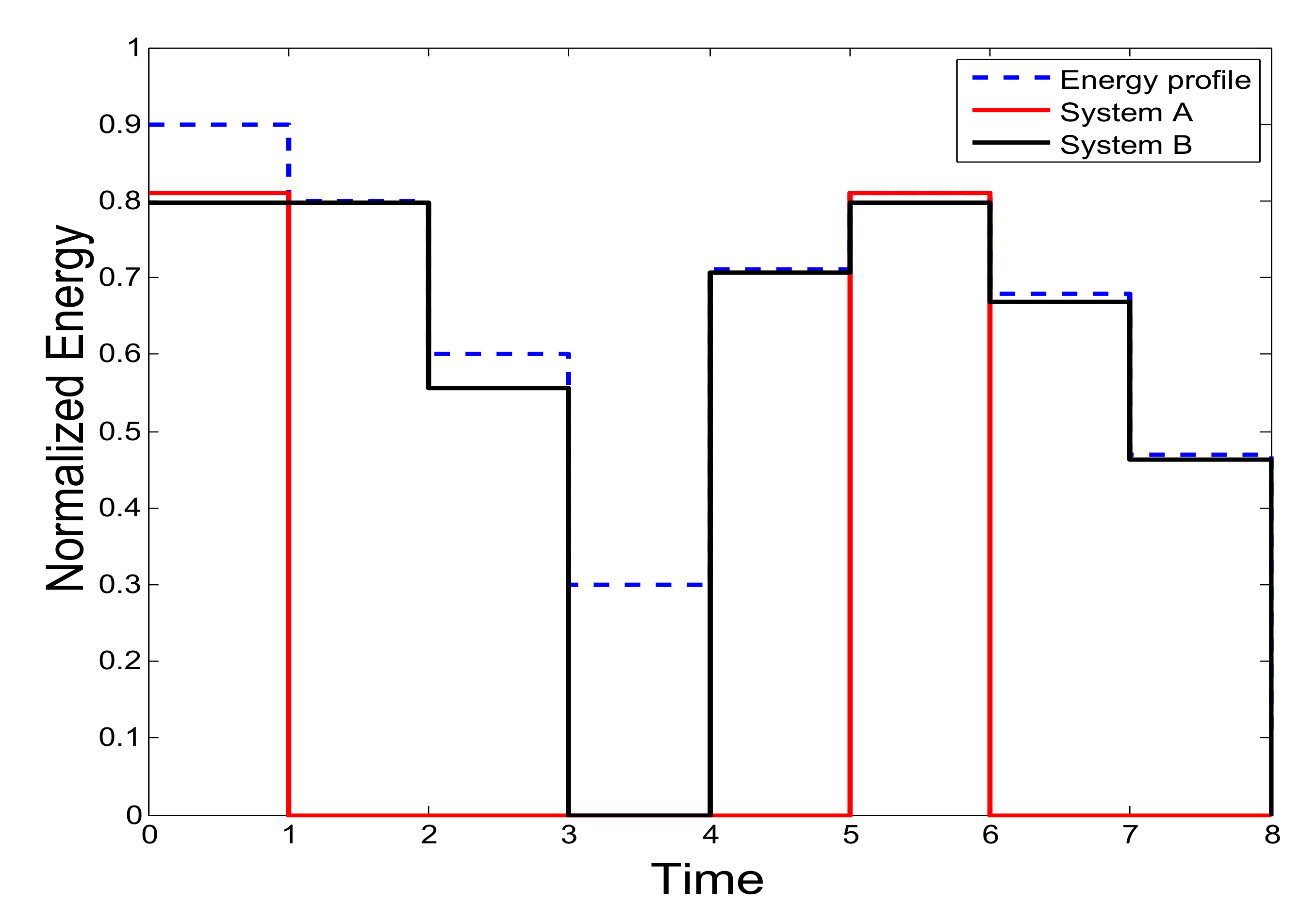
3.1. Research Hypothesis

The designers of limited-energy Internet of Things (IoT) applications, such as wireless sensor nodes (WSNs), have several design trade-offs when selecting the most suitable ANN for their application. Given that approximated ANNs designs are reported in the literature with various energy-accuracy flavors, the limited-energy applications designers usually select the ANN that exhibits moderate energy consumption and acceptable accuracy.

In this research work, the following research question is investigated “Is it possible to reconfigure the application with different ANN flavors adaptively based on the available energy budget? and if yes, how much energy is saved?”. In other words, this work attempts to provide an energy-driven adaptive IoT application platform that is reconfigured with a specific ANN design according to the available battery energy at the expense of accuracy degradation. The ANN is used as a case study to answer this research hypothesis question with the application of the Partial Dynamic Reconfiguration feature of the FPGA; however, any design that has energy trade-offs can be used following the same work flow and methodology.

Figure 2 displays a block diagram of the target limited-energy application that consists of static modules and dynamic modules. The static modules are fixed and performing other functions of the application such as decision-making circuits. The dynamic modules are reconfigured as follows. The battery energy sensor determines the battery energy level and accordingly, the PDR controller reconfigures the dynamic modules of the application with the corresponding ANN. For example, assuming that ANN1 has the highest energy consumption with the highest accuracy and ANN5 has the lowest energy consumption with the lowest accuracy. The reconfiguration methodology should be as follows. (1) when the battery energy level is from 1% to 20%, ANN5 should be selected, (2) when the battery energy level is from 21% to 40%, ANN4 should be selected, (3) when the battery energy level is from 41% to 60%, ANN3 should be selected, (4) when the battery energy level is from 61% to 80%, ANN2 should be selected, and (5) when the battery energy level is from 81% to 100%, ANN1 should be selected. The number of reconfigurations depends on the available ANN flavors and correspondingly, the energy levels values. In addition, the energy levels might be non-uniform in some applications depending on the ANN design energy trade-offs.

3.2. Approximate Computing Techniques for Energy Savings

3.2.1. Precision Scaling

Precision scaling is a widely used approximate computing technique [7,14,15]. For power/energy savings, fixed-point is used in implementing neural networks instead of the computationally expensive floating point. Precision scaling is carried out by forcing the least significant bits (LSBs) of fixed-point operands to zero (Software precision scaling) or by implementing the design with reduced word length (hardware precision scaling). Both techniques reduce the energy consumption by decreasing the switching activity. Precision scaling of the weights and inputs affects the consumed power of all the components of the neuron unit such as the multiplier, the accumulator, and the activation function. Hardware precision scaling also affects the size and the consumed power of the memory required for storing weights and intermediate results.

A fixed-point word length of 32 bits results in the same accuracy as the floating-point word implementation. However, it is found from the experimental results that a 12-bit word length is enough to achieve the same accuracy as that of the 32-bit word length in case of the MNIST dataset, and an 8-bit word length is enough to achieve the same accuracy as that of the 32-bit word length in case of the SVHN dataset. Reducing the word length lower than these lengths (i.e., 12-bit for the MNIST dataset case and 8-bit for the SVHN dataset case) achieves a higher saving in energy at the expense of accuracy degradation.

For a given word length, the full dynamic range of the bits should be used to achieve the highest accuracy for this specific word length configuration. This requires a good selection of the integer and fraction portions of the fixed-point word length. For instance, when using Sigmoid or Tanh activation functions, the inputs of the neuron do not exceed ±1. Consequently, the integer length of the operands of the neuron unit is selected to be 2-bits, including the sign bit.

3.2.2. Inaccurate Arithmetic

Neural networks involve thousands of arithmetic operations such as multiplications and accumulations. Using inaccurate arithmetic operations introduces some errors which are tolerated due to neural networks resiliency. However, using this inaccurate arithmetic operations saves a big chunk of energy. A multiplier is one of the power-hungry units in digital neural networks. Many approximate multipliers are proposed in the literature [12,16,17,18]. In this paper, the signed truncated multiplier proposed in [18] is used. This signed truncated multiplier consumes less power than accurate multipliers by summing an optimized partial products matrix (PPM). The idea of the signed truncated multiplier is that it reduces the number of bits of the result by truncating part of the fraction bits and then compensating the truncated bits to ensure a reasonable accuracy. Therefore, it is a good option to use to save area and power.

Approximate adders are used also to reduce the power consumption, however, they have smaller impact on the energy savings than approximate multipliers. In this paper, instead of using an approximate adder, a truncated accumulation is used then accumulating the whole output of the multiplier (i.e., the output of the multiplier is truncated to the specified word length, then the accumulation operation is performed). This also reduces the size/power of the needed accumulator and has an insignificant impact on accuracy.

3.2.3. Computation Skipping

In many applications or datasets, the number of zero, or near zero, valued neuron inputs is high. Moreover, using precision scaling significantly increases the number of zero-valued inputs. Also, using Rectified Linear Unit (RELU) layers, which force the negative valued layer outputs to zero, participates in increasing the number of zeros in the system. By detecting these zeros, unnecessary computations are avoided by using computation skipping.

In the proposed EANN system, a zero detecting hardware is used which indicates if the upcoming data to the neuron unit is zero and accordingly, skips the computation. This is done by disabling the neuron unit that has zero inputs and skipping the memory read of its associated weights. This procedure decreases the switching activity of the EANN system without any loss in accuracy.

3.2.4. Neurons Skipping

To further decrease energy, some neurons in the hidden layers are skipped and all operations associated with them are not performed. For example, in a system with 10 physical neuron units running on MNIST dataset with a single hidden layer of 100 neurons, if ten of the 100 hidden neurons are skipped, 7860 (i.e., the number of inputs ×10) Multiply-and-Accumulate (MAC) operations and memory access operations are not performed reducing the time and energy needed for inference.

In contrast to computation skipping which avoids unnecessary computations and has no effect on accuracy, neurons skipping does have an impact on accuracy, but saves more energy. To reduce the impact of neuron skipping on accuracy, the skipped neurons should be selected carefully. The selected neurons should be the most resilient ones so that skipping them has the smallest effect on the inference.

A neurons resilience ranking method has been proposed in [3]. This method depends on backpropagating the error at the output layer for each instance of the training set and calculates the average error contribution for each neuron to identify the least contributing neurons to the output error. In this work, the following hardware friendly method is used.

Given that the output of each neuron is calculated by MAC operations between the neuron inputs and the associated weights, and that all neurons in the same layer share the same inputs, a neuron whose associated weights have the smallest average magnitude is more likely to have near zero MAC result. Thus, the neuron resilience ranking is done according to the average magnitude of the associated weights of each neuron.

The associated weights of the most resilient neurons are placed at the top of the weights memory so that if 10 neurons are selected to be skipped to reduce the consumed energy, the controller skips the weights of the first ten neurons in the memory and starts reading normally after them. Skipping of some neurons in a neural network layer also affects the following layer. The input to the following layer from a skipped neuron is set to $g\left(zero\right)$ where $g\left(x\right)$ is the activation function of the previous layer, which equals to zero when using Tanh or RELU functions, allowing more energy reduction if computation skipping is used, and $g\left(x\right)$ equals to 0.5 when Sigmoid is used.

3.2.5. Activation Function Approximations

Another technique for energy saving is the adoption of approximate implementation of the activation functions. For example, instead of implementing the hardware costly exponential operation for implementing the Sigmoid function, a Piece-Wise Linear (PWL) approximation is used to reduce the consumed power. Using linear activation functions such as RELU is viewed also as power reduction method. RELU hardware is much smaller compared to Sigmoid as it requires only compared to zero. However, as the RELU function passes any value above zero as it is, this requires larger arithmetic units in the following layers because the integer length of the fixed-point representation is increased due to MAC operations. Instead of using bigger hardware, a truncated versions of the RELU outputs are used to save power at the cost of reduced accuracy.

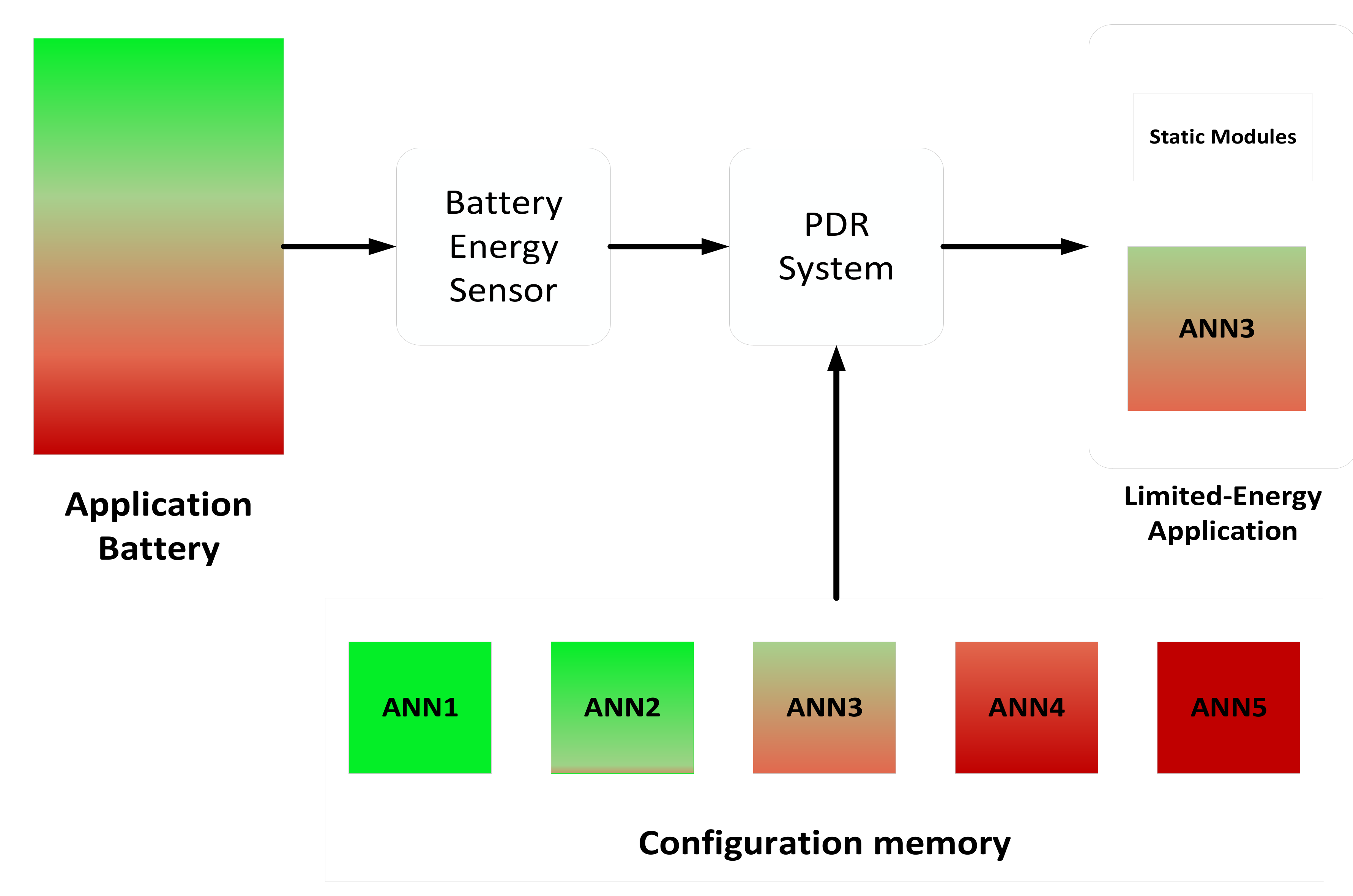
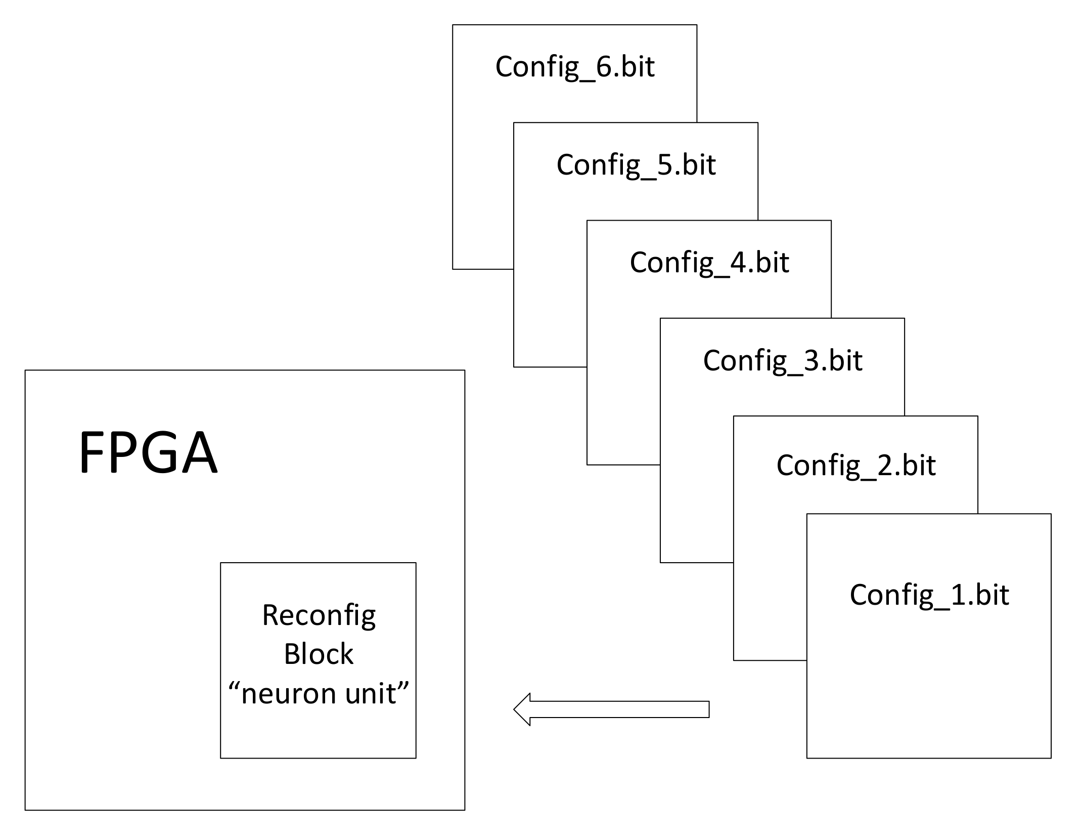
3.3. Partial Dynamic Reconfiguration (PDR)

Partial Dynamic Reconfiguration is a very powerful technique in hardware implementations using FPGAs (Field Programmable Gate Arrays). The new advantage about dynamic reconfiguration is that it allows another degree of freedom to reconfigure a specific part of the FPGA hardware in the run-time according to the application needs.

In general, an FPGA consists of two main parts: the hardware elements that it supports and the configuration memory that holds the bitstream (binary) files used to program that hardware. The hardware layer in FPGA contains the basic infrastructure that any design can be implemented using it by changing the connections and contents of it. These hardware resources are mainly Lookup Tables (LUTs), flip-flops and memory blocks. The configuration memory in FPGA is used to store the information needed to configure the hardware elements, the routing details between the different resources, the values stored in the LUTs that implement a specific function, the reset values of the flip-flops used in the design, and all other details needed for a proper operation. Thus, to change the functionality done by FPGA, one must change the configuration file and when loaded on FPGA a new hardware with a new function is in operation.

The term partial indicates the ability to change part of the design while maintaining the rest of the design unchanged. Second, the term dynamic means that the reconfiguration process is performed at the run-time without turning the FPGA device OFF.

There are many advantages for using the partial dynamic reconfiguration. It makes it possible to have more than one hardware implementation of a function and to reconfigure one of them base on the application needs. Thus, the PDR is the best choice in an adaptive hardware design that must respond according to a changing environment.

4. Experimental Results

4.1. Experimental Setup

As a proof of concept, the idea to dynamically reconfigure the hardware of an artificial neural network is tested using two different datasets “MNIST and SVHN” and a different neural network architecture is designed for each dataset.

MNIST (Modified National Institute of Standards and Technology) database is handwritten digits from 0 to 9. It has a training set of 60,000 samples, and a testing set of 10,000 samples [19]. SVHN (Street View House Number) database is a real-world images of cropped digits. It has 73257 training samples and 26032 testing samples [20].

Each one of the previous datasets has a different complexity level. Thus, to obtain a reasonable accuracy from them, each dataset is tested on a different network structure. MNIST is tested on a network structured as 785-100-10 (i.e., 785 input neurons, 100 hidden-layer neurons, and 10 output neurons), and its highest accuracy is 97.92%. SVHN is tested on a network structured as 1025-300-300-10 (i.e., 1025 input neurons, 300 first hidden-layer neurons, 300 second hidden-layer neurons and 10 output neurons), and its highest accuracy is 80.58%.

To implement such networks on the hardware, one can implement all the neurons physically. The second option is to implement certain number of neurons physically and reuse them in the calculations of other neurons. In this paper, the second approach is adopted as this work targets limited-energy applications. Ten physical neurons are implemented on the hardware and they are reused to obtain the results of all neurons. Thus, the first ten neuron operations are carried out and their results are saved in a hidden memory, then the second ten neuron operations are carried out, and so on until all the first layer neuron operations are carried out. The output of the first hidden layer is saved in the hidden memory and is used as the input to the output layer. Then, the same ten physical neurons are used to carry out the computation of the output layer.

Accuracy results are obtained on the software level using Python, and then verified on the hardware level using the designed hardware networks. Power, area and reconfiguration time are obtained by Vivado Design Suite-Xilinx version 2016.4 on the “ZYNQ Ultra-Scale+” MPSoC FPGA. The power is estimated using Vivado software tool by using the simulation activity files to estimate the dynamic power consumption of the design.

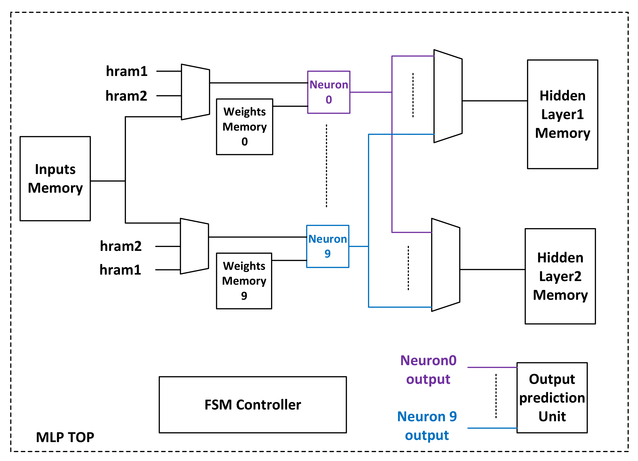
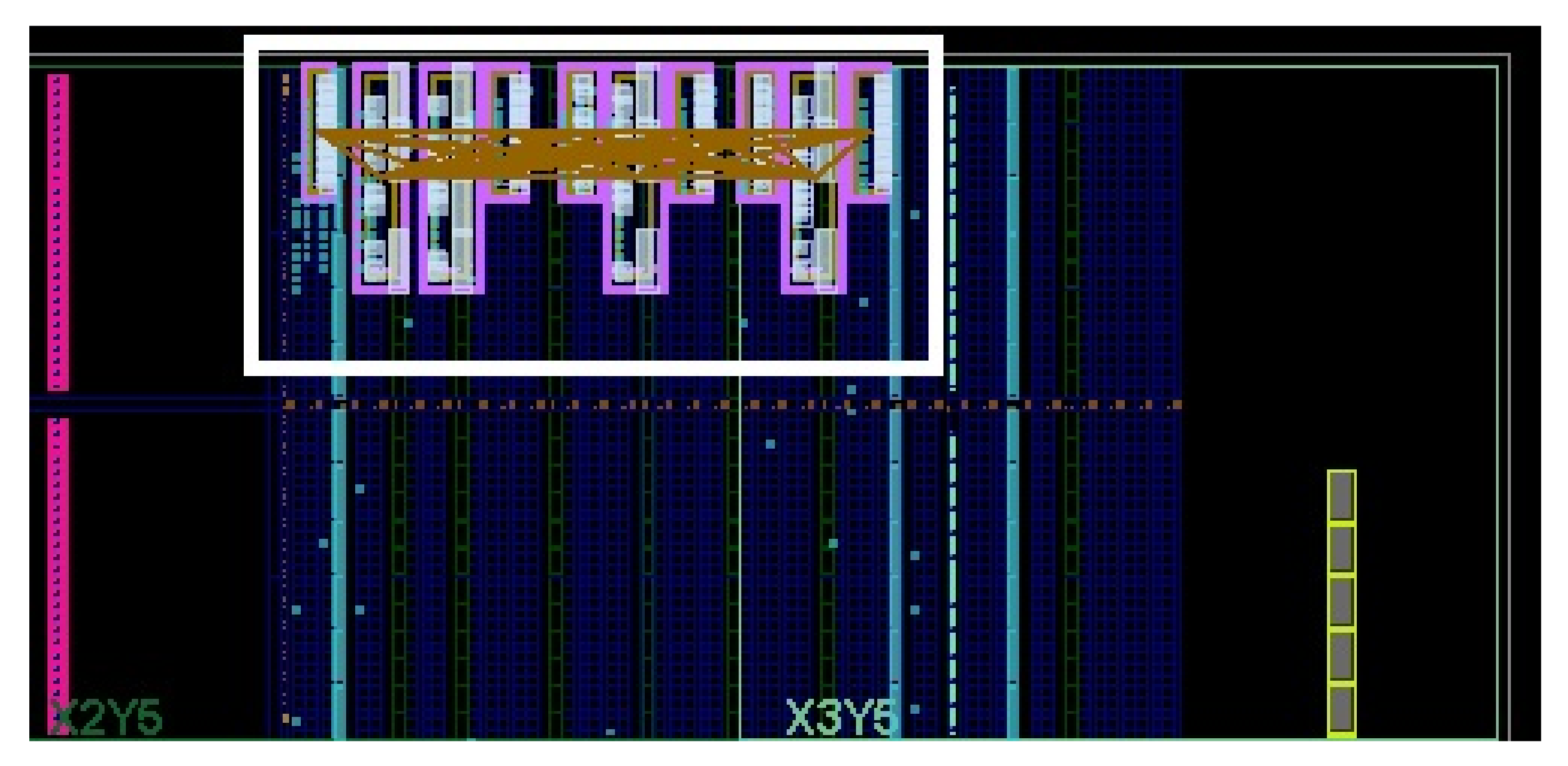
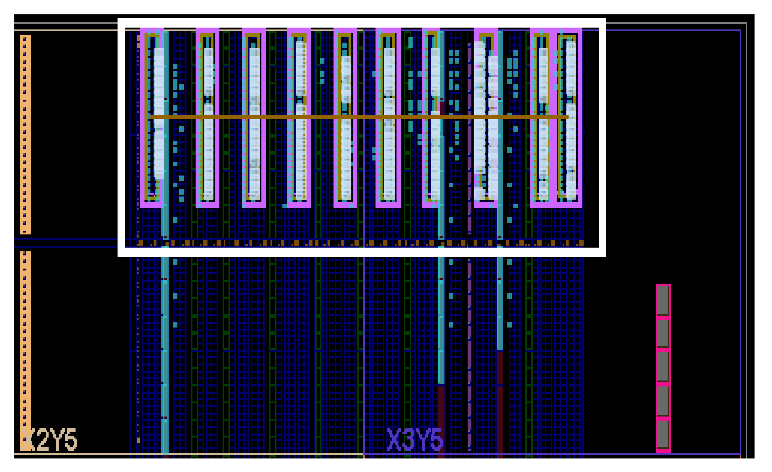
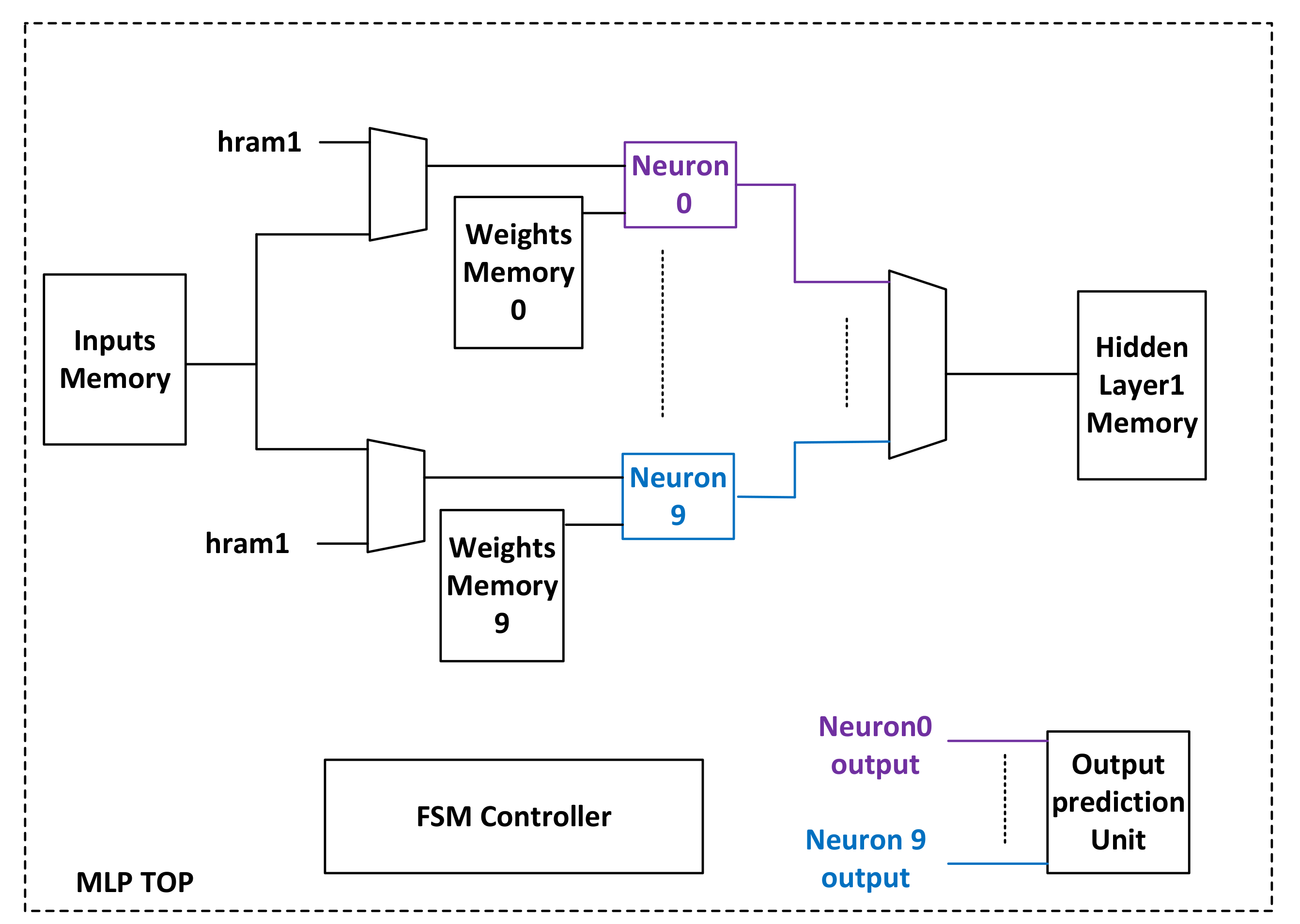
4.2. Block Diagram and Hardware Implementation of the Neural Network Used for MNIST Dataset

The system top level of the neural network used in MNIST dataset consists of two memory blocks one to store the inputs which is the “inputs memory” in Figure 3, and the other to store the intermediate results of the first hidden layer which is the “HiddenLayer1 Memory” in Figure 3. The content of HiddenLayer1 memory is then used as an input to the output layer. The system has ten physical neurons referred to as Neuron0 to Neuron9 in the figure. There is one memory attached to each neuron to hold the weights associated with this neuron that is obtained from the training phase. A multiplexer is also attached to each neuron input to select whether the input is taken from the input memory or from the hidden memory. The neuron input is from the input memory only for the first layer neurons and from the hidden memory for other layers. In Figure 3, hram1 refers to the output of “HiddenLayer1 Memory”. The output prediction unit is used in the output layer to predict the result of a certain input. A main control finite state machine “FSM controller” exists to control the data movement between the blocks, to provide control signals to all blocks such as memories read and write enables, registers resets, multiplexer selections and counters increment and decrement signals.

4.3. Block Diagram and Hardware Implementation of the Neural Network Used for SVHN Dataset

The system top level for the neural network used for SVHN dataset consists of three memory blocks one to store the inputs similar to the one used in the MNIST block diagram which is the “inputs memory” in Figure 4, and two memories to store the intermediate results of the first hidden layer and the second hidden layer referred to in Figure 4 as “HiddenLayer1 Memory” and “HiddenLayer2 Memory”, respectively. The first hidden memory is used to store the outputs of the first hidden layer and as an input to the second hidden layer. The second hidden memory is used to store the outputs of the second hidden layer and as an input to the output layer. In Figure 4, hram1 refers to the output of “HiddenLayer1 Memory”, and hram2 refers to the output of “HiddenLayer2 Memory”.

The output prediction unit is used in the output layer to predict the result of a certain input. A main control finite state machine "FSM controller" exists to control the data movement between the blocks, to provide control signals to all blocks such as memories read and write enables, registers resets, multiplexer selections and counters increment and decrement signals.

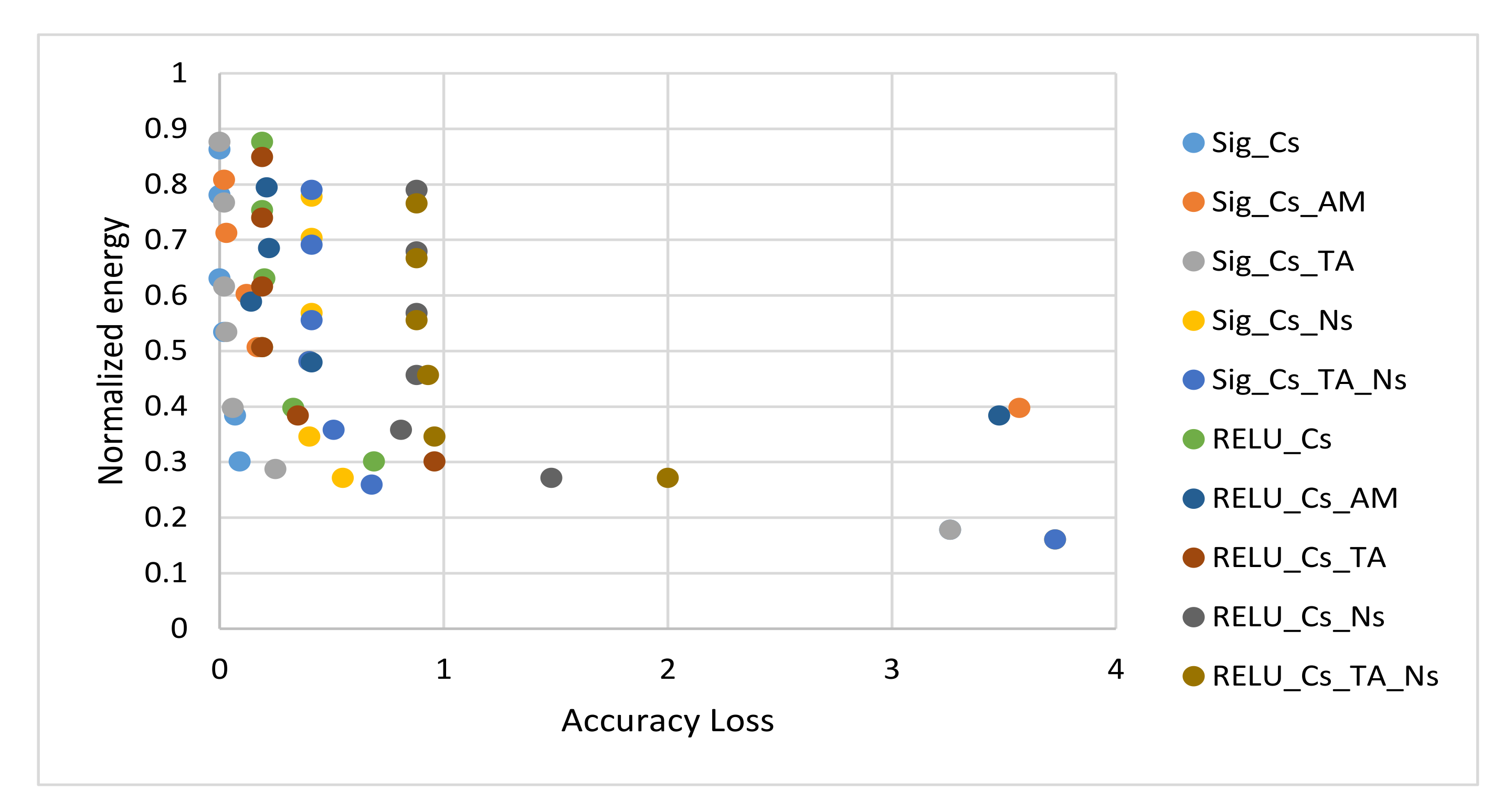
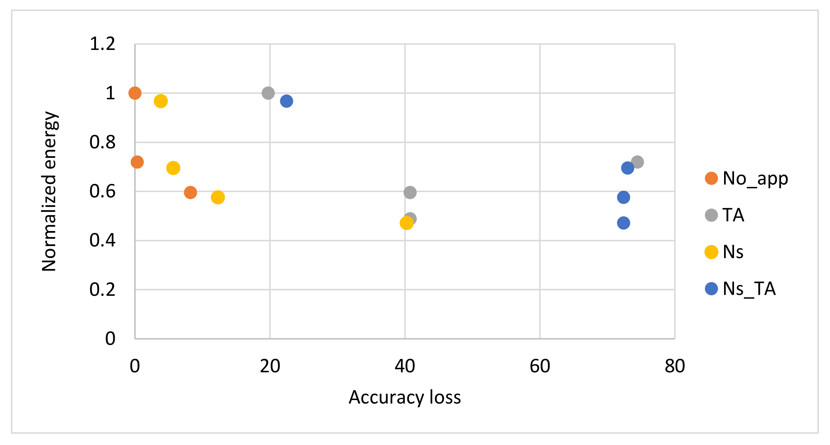
4.4. Simulation Results and Discussions

Applying the approximations described above (i.e., approximate multiplier, truncated accumulation, approximate activation function, computation skipping and neuron skipping) with different word lengths results in a wide range of energy levels with different accuracy loss. The energy is obtained using the following formula:

$$Energy=\frac{n\times p}{f}$$

(1)

where n is the number of cycles, p is the power in mW and f is the frequency of operation. The accuracy loss is calculated as a percentage decrease from the highest obtained accuracy when 32-bits word length is adopted.

To explain the energy formula, the network of MNIST dataset is taken as an example. It consists of 785 input neurons, 100 hidden neurons, and 10 output neurons. It is a fully connected network, all the layer outputs are used as inputs to the following layer. The output of each neuron is calculated as the weighted sum of the neuron inputs passed by the activation function. To get the output for a certain input from such a network, it is needed to perform 78,500 multiply-and-accumulate (MAC) operations in the first layer and 1000 operations in the output layer. Since the hardware uses only 10 physical neurons, then the number of cycles (n) to finish the whole computation is the total number of needed operations divided by the physical neurons count and equals 79,500/10 = 7950 cycles.

For the MNIST dataset, the energy is normalized to the highest obtained energy. The highest consumed energy is obtained when the ANN operates using word length of 12-bits (because experimental results show that the 12-bits word length results in the same accuracy as the 32-bits and the floating point in case of the MNIST dataset) and using computation skipping technique, and this implementation (i.e., 12-bits and computation skipping) also gives the highest accuracy. For the SVHN dataset, the energy is also normalized to the highest energy obtained. The highest consumed energy is obtained when the ANN operates using word length of 8-bits (because experimental results show that the 8-bits word length results in the same accuracy as the 32-bits and the floating point in case of the SVHN dataset) and without using any other approximation technique, and this configuration also gives the highest accuracy. The accuracy loss is calculated for both datasets as a percentage decrease from the highest obtained accuracy.

Figure 5 and Figure 6 show the different approximations for MNIST and SVHN dataset, respectively. Each point in these figures represents a certain configuration (i.e., using one or more approximation) using a certain word length (i.e., changing the word length from 12-bits and down for the MNIST and from 8-bits and down for the SVHN given that the 12-bits and the 8-bits provide the same accuracy as the floating point and the 32-bit word length for MNIST and SVHN, respectively). These points are used later as a searching space for the best configuration to conform with the available energy budget given from the system level.

Using Sigmoid and RELU as activation functions for MNIST results in different values in terms of accuracy and energy. Since saturation or truncation of the RELU outputs is used to save power at the cost of reduced accuracy, RELU always gives worse results than Sigmoid for the same approximation. As shown in Figure 7, for different word lengths, Sigmoid always has almost the same energy of RELU with lower accuracy loss. Accordingly, all RELU points are excluded at the configuration selection step. The final configurations that are used as a searching space for the MNIST dataset to get the adaptive energy are displayed in Figure 8.

In the MNIST dataset, the input by nature contains many pixels with zero value so applying computation skipping in this case helps in decreasing the energy while achieving the same accuracy. Figure 9 shows the difference between using computation skipping and not using it in terms of accuracy loss and consumed energy. Therefore, computation skipping is used with all other MNIST approximation techniques. In case of SVHN, since it contains pictures from a real world, there are few zero-valued pixels exist in these images and accordingly, the computation skipping technique is not used.

4.5. Proposed Algorithm and Configurations Selection

To introduce the proposed energy adaptive neural network (EANN) algorithm, suppose the use of a battery-powered application. In these applications, if the voltage level that feeds the hardware circuits falls below a certain level, it causes the system to power OFF. If the profile of the voltage drop with time is known, then the amount of the available energy for the system to operate for a certain amount of time is also known. The EANN system makes use of this information to adapt its hardware units to operate with a lower energy at a lower accuracy mode, thus the battery lifetime is increased.

As shown in Figure 10, the neuron unit has more than one hardware implementation due to different approximations used. Each neuron configuration has different area, power and accuracy flavors. These different configurations are used to adapt to the given energy level. The logic in FPGA is divided into two parts: static part which models the memory used for storing weights and the top-level circuits, and dynamic (reconfigurable) part which is the neuron unit. During reconfiguration, the static part remains functioning and the dynamic part changes without turning the system OFF. This allows the EANN system to choose among the different configurations to adapt itself to meet the energy constraint.

Table 1. Power and accuracy regions for the MNIST dataset.

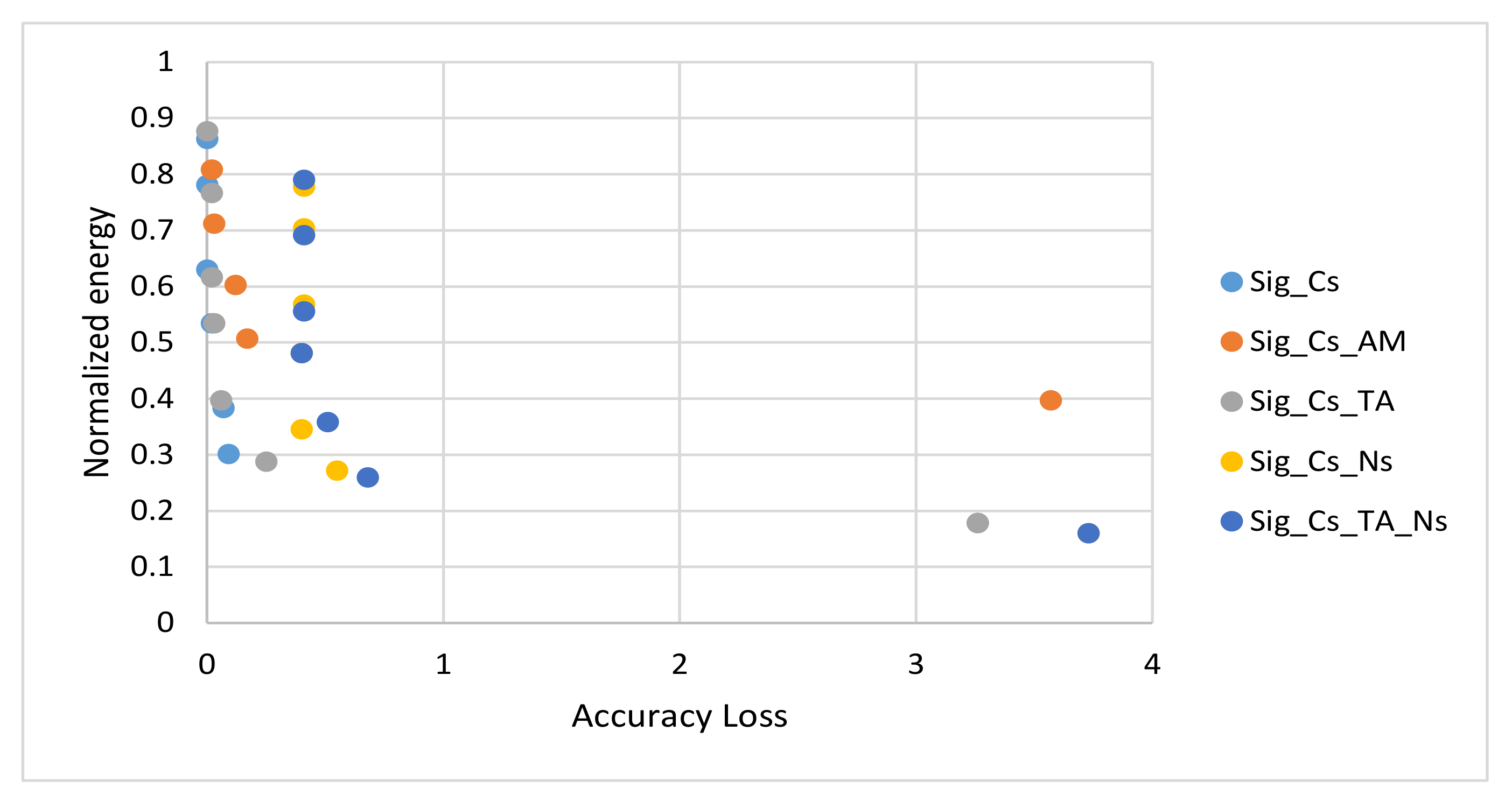
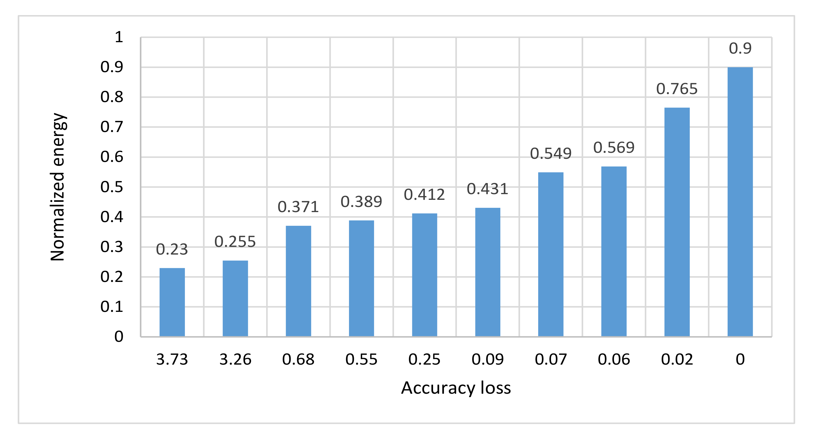
Normalized Energy	Accuracy Loss%	Configurations
0.230	3.73	Cs_TA_Ns_4
0.255	3.26	Cs_TA_4
0.371	0.68	Cs_TA_Ns_6
0.389	0.55	Cs_Ns_6
0.412	0.25	Cs_TA_6
0.431	0.09	Cs_6
0.549	0.07	Cs_8
0.569	0.06	Cs_TA_8
0.765	0.02	Cs_10
0.9	0	Cs_12

Cs: Computation skipping, Ns: Neuron skipping, TA: Truncated Accumulation.

shows the normalized energy and accuracy loss of different configurations in case of MNIST dataset. In this table, each row indicates a certain configuration, its accuracy loss, and its normalized energy. For example, the first row means that this configuration uses computation skipping, truncated accumulation, neuron skipping and word length of 4.

For the MNIST dataset, the energy is divided to ten levels in this test case as shown in Figure 11. In the EANN system, there is a sensing circuit that could determine the available energy, then the comparators select the nearest level to that energy level. After choosing the best-fit energy level, the suitable configuration that fits with this energy budget is selected from Table 1. For example, if the sensing circuit outputs energy greater than or equal to 0.9 (i.e., 90% of the total energy of the unapproximated neural network), then the proposed EANN system operates with highest accuracy and zero accuracy loss (whereas the highest energy ANN is adopted). From Table 1, the configuration that is selected in this case is the neuron unit that supports computation skipping using word length of 12. If the energy drops to 0.765 (i.e., 76.5% of the total energy of the unapproximated neural network), then the second energy level with accuracy loss 0.02% is selected and the FPGA is reconfigured. The configuration that is used in this case is the neuron unit that supports computation skipping and truncated accumulation with word length 10.

Table 2. Power and accuracy regions for the SVHN dataset.

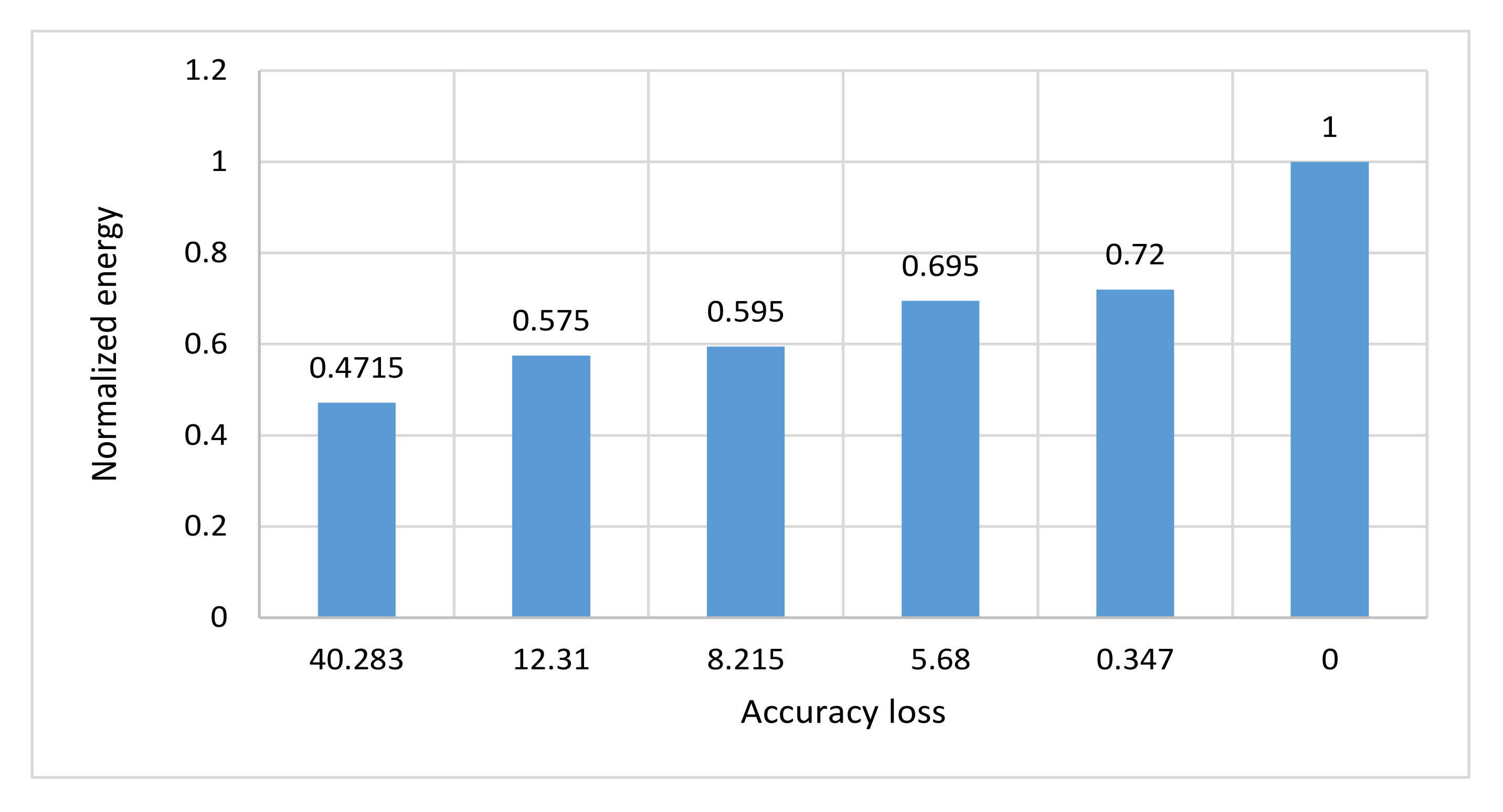
Normalized Energy	Accuracy Loss%	Configurations
0.472	40.3	Ns_4
0.575	12.3	Ns_5
0.595	8.2	NoApp_5
0.695	5.7	Ns_6
0.720	0.35	NoApp_6
1	0	NoApp_8

NoAPP: No approximations, Ns: Neuron skipping.

shows the normalized energy and accuracy loss of different configurations in case of SVHN dataset. In this table, each row indicates a certain configuration, its accuracy loss, and its normalized energy. For example, the first row means that this configuration uses neuron skipping approximation and word length of 4.

For the SVHN dataset, the energy is divided to six energy levels as shown in Figure 12. Here in this case, if the sensing circuit outputs full energy, then the proposed EANN system operates with highest performance and zero accuracy loss. From Table 2, the configuration that is selected in this case is the neuron unit with no approximation using word length of 8. If the energy drops to 0.72 (i.e., 72% of the total energy of the unapproximated neural network), then the second energy level with accuracy loss 0.347% is selected and the FPGA is reconfigured. The configuration that is used in this case is the neuron unit with no approximation and word length 6.

None of the selected configuration has approximate multiplier in its implementation. The reason is that any configuration contains approximate multiplier has higher accuracy loss than other configurations with the same energy.

The cost of the reconfigurability is the reconfiguration time, which is the time consumed by the dynamic part to change from one configuration to the other. Another disadvantage of PDR is that the area occupied on the FPGA is the area of the biggest configuration. However, the strength of the proposed energy adaptive technique is that the EANN system does not shut down when it fails to achieve the highest accuracy. Instead, it keeps operating with the lower available energy budget at the expense of lower accuracy.

To compare between the proposed EANN system and the conventional ANN systems, suppose that system A (a conventional ANN system) needs a normalized energy of 0.8 (i.e., 80% of the total energy of the unapproximated neural network) to work with the best performance and no accuracy loss. In system A, if the energy falls below 0.8, the system turns OFF. In the proposed EANN system B, if it is given 0.8 energy, it works with the best performance and no accuracy loss. However, in system B (the proposed EANN system) if the energy falls below 0.8 and becomes 0.6 (i.e., 60% of the total energy of the unapproximated neural network), it reconfigures its units and works with the available energy budget with accuracy loss of 0.09% which is a slight decrease in accuracy but helps in reducing the consumed energy.

If there is always available energy of 0.8, system A and B are of the same performance. When system B has energy less than 0.462 (i.e., 46.2% of the total energy of the unapproximated neural network), it also turns OFF. The main drawback of system B is that it occupies a total area equivalent to conventional ANN system (i.e., system A) even if the available energy is between 0.4 and 0.8. However, from energy perspective, system B adapts itself to the available energy budget trading off the accuracy for energy adaptively. System B is the best choice if the available energy is always changing and not fixed. The overhead in system A is the reconfiguration time among the different modules. Figure 13 shows the difference between the proposed EANN system and the conventional system that targets maximum accuracy over the time from the operation perspective.

Figure 14 shows the design floorplanning on “ZYNQ UltraScale+” MPSoC for the SVHN dataset hardware implemented neural network. Figure 15 shows the design floorpanning for the MNIST dataset hardware implemented neural network. The reconfigurable partitions of this design are the 10 physical neurons, they are floorplanned to accommodate the maximum hardware needed among all configurations. The most important benefit of PDR is that there is no need to switch the system off to perform the reconfiguration task. Instead, it takes place during the run-time. This is a good advantage of the PDR technique since, in some applications such as the wireless image sensor of precision agriculture, it is required to keep the system alive and functioning during the whole experiment time. The trade-off is sacrificing some accuracy due to reconfiguration. The reconfigurability of the FPGA allows use of multiple implementations of the same module that does the same functionality, but with different accuracy and energy consumption.

Partial dynamic configuration saves much area. It is not needed to implement all the possible configurations on the system and build a controller to perform the switching task between them. As shown in

Table 3. Area, Power and accuracy results for SVHN configurations.

Configuration	Area		Power(mW)	Accuracy(%)
	CLB	BRAM
WL_8	4297	161.5	121	80.58
WL_6	3015	121.5	87	80.30
WL_5	2489	101.5	72	73.96
WL_4	2173	81.5	59	47.73

, for the SVHN dataset, if all possible configurations of the neuron unit are implemented on the board, this consumes much area and power. The area needed to implement all configuration is about 11,974 CLBs and 466 BRAMs and consumes a total power of about 339 mW. The area needed to implement EANN system is the area of the largest reconfiguration module (highest accuracy) configuration and the area of the static routing connections which is about (4297 CLBs and 161.5 BRAMs). This indicates that the EANN system achieves about 2.8X area and power reduction.

In case of the MNIST dataset as shown in

Table 4. Area, Power and accuracy results for MNIST configurations.

Configuration	Area		Power(mW)	Accuracy(%)
	CLB	BRAM
Cs_12	7369	31	46	97.92
Cs_10	5715	26	39	97.90
Cs_TA_8	3736	21	28	97.86
Cs_8	3980	21	29	97.85
Cs_6	2728	15.5	22	97.83
Cs-_TA_6	2606	15.5	21	97.67
Cs_TA_4	1853	10.5	13	94.66

, if all configurations are implemented on the same board, the area needed is about(27987 CLBs and 140.5 BRAMs) and consumes a total power of about 198 mW. The area needed to implement EANN system is the area of the largest reconfiguration module (highest accuracy) configuration and the area of the static routing connections which is about (7369 CLBs and 31 BRAMs). This indicates that the EANN system achieves about 3.8X area and around 4X power reduction.

The overhead of using PDR is the reconfiguration time needed to load one configuration of the neuron unit and the need for external memory to store the partial bit files of all neuron unit configurations.

$$Reconfiguration time=(Total Partial Bit\_Stream File Size/Throughput).$$

(2)

The commonly used access port for PDR is the Internal Configuration Access Port (ICAP), and its throughput is 400 MB/sec. The reconfiguration time depends on the area of the partition and the speed of the PDR controller. Using the “ZYNQ UltraScale+” MPSoC, the maximum reconfiguration time to reconfigure the ten physical neurons is 3.7625 ms for the MNIST dataset, and 2.7825ms for the SVHN dataset. This reconfiguration time is very short if it is compared to the expected rate of energy changes. This assumption is emphasized by noting that the energy level changes are mainly due to the harvested energy variations or the battery energy level fluctuations, which are usually in the order of seconds.

5. Conclusions

This paper represents a new method to make the neural network energy adaptive using partial dynamic reconfiguration. The proposed EANN system uses variety of network approximation techniques such as precision scaling, approximate multipliers, truncated accumulation, approximate activation function, computation skipping and neuron skipping. The idea is tested using two datasets, SVHN and MNIST. A combination of different configurations is then used to achieve a wide range of energy levels to adapt to the available energy budget in the proposed EANN system at the expense of degraded accuracy. Using the partial dynamic reconfiguration technique, the proposed EANN system selects one of the configurations at a time to adapt to the energy budget at the expense of lower accuracy. With the proposed approach, the EANN system is always functioning with variable accuracies according to the available energy level rather than the ON-OFF conventional system behavior.

References

- Kalogirou, S.A. Applications of artificial neural-networks for energy systems. Appl. Energy 2000, 67, 17–35. [Google Scholar] [CrossRef]
- Janardan, M.; Indranil, S. Artificial neural networks in hardware: A survey of two decades of progress. Neurocomputing 2010, 74, 239–255. [Google Scholar]
- Venkataramani, S.; Ranjan, A.; Roy, K.; Raghunathan, A. AxNN: Energy-efficient neuromorphic systems using approximate computing. In Proceedings of the IEEE/ACM International Symposium on Low Power Electronics and Design (ISLPED), La Jolla, CA, USA, 11–13 August 2014; pp. 27–32. [Google Scholar]
- Zhang, Q.; Wang, T.; Tian, Y.; Yuan, F.; Xu, Q. ApproxANN: An approximate computing framework for artificial neural network. In Proceedings of the Design, Automation & Test in Europe Conference & Exhibition (DATE), Grenoble, France, 9–13 March 2015; pp. 701–706. [Google Scholar]
- Jaeha, K.; Duckhwan, K.; Saibal, M. A power-aware digital feedforward neural network platform with backpropagation driven approximate synapses. In Proceedings of the IEEE/ACM International Symposium on Low Power Electronics and Design (ISLPED), Rome, Italy, 22–24 July 2015; pp. 85–90. [Google Scholar]
- Sarwar, S.S.; Venkataramani, S.; Raghunathan, A.; Roy, K. Multiplier-less artificial neurons exploiting error resiliency for energy-efficient neural computing. In Proceedings of the Design, Automation & Test in Europe Conference & Exhibition (DATE), Dresden, Germany, 14–18 March 2016; pp. 145–150. [Google Scholar]
- Mrazek, V.; Sarwar, S.S.; Sekanina, L.; Vasicek, Z.; Roy, K. Design of power-efficient approximate multipliers for approximate artificial neural networks. In Proceedings of the 35th International Conference on Computer-Aided Design, Austin, TX, USA, 7–10 November 2016. [Google Scholar]
- Duckhwan, K.; Jaeha, K.; Saibal, M. A power-aware digital multilayer perceptron accelerator with on-chip training based on approximate computing. IEEE Trans. Emerg. Top. Comput. 2017, 5, 164–178. [Google Scholar]
- Gerald, E. Reconfigurable computer origins: The UCLA fixed-plus-variable (F + V) structure computer. IEEE Ann. Hist. Comput. 2002, 24, 3–9. [Google Scholar]
- Kamaleldin, A.; Hosny, S.; Mohamed, K.; Gamal, M.; Hussien, A.; Elnader, E.; Shalash, A.; Obeid, A.M.; Ismail, Y.; Mostafa, H. A reconfigurable hardware platform implementation for software defined radio using dynamic partial reconfiguration on Xilinx Zynq FPGA. In Proceedings of the IEEE 60th International Midwest Symposium on Circuits and Systems (MWSCAS), Boston, MA, USA, 6–9 August 2017; pp. 1540–1543. [Google Scholar]
- Sparsh, M. A survey of techniques for approximate computing. ACM Comput. Surv. (CSUR) 2016, 48, 1–33. [Google Scholar]
- Cong, L.; Jie, H.; Fabrizio, L. A low-power, high-performance approximate multiplier with configurable partial error recovery. In Proceedings of the Design, Automation & Test in Europe Conference & Exhibition (DATE), Dresden, Germany, 24–28 March 2014; pp. 1–4. [Google Scholar]
- Uroš, L.; Patricio, B. Applicability of approximate multipliers in hardware neural networks. Neurocomputing 2012, 96, 57–65. [Google Scholar]
- Moons, B.; Brabandere, B.D.; Gool, L.V.; Verhelst, M. Energy-efficient convnets through approximate computing. In Proceedings of the IEEE Winter Conference on Applications of Computer Vision (WACV), Lake Placid, NY, USA, 7–9 March 2016; pp. 1–8. [Google Scholar]
- Panda, P.; Sengupta, A.; Sarwar, S.S.; Srinivasan, G.; Venkataramani, S.; Raghunathan, A.; Roy, K. Cross-layer approximations for neuromorphic computing: From devices to circuits and systems. In Proceedings of the 53rd Annual Design Automation Conference, Austin, TX, USA, 5–9 June 2016; pp. 1–6. [Google Scholar]
- Parag, K.; Puneet, G.; Milos, E. Trading accuracy for power with an underdesigned multiplier architecture. In Proceedings of the 24th Internatioal Conference on VLSI Design, Chennai, India, 2–7 January 2011; pp. 346–351. [Google Scholar]
- Mahdiani, H.R.; Ahmadi, A.; Fakhraie, S.M.; Lucas, C. Bio-inspired imprecise computational blocks for efficient VLSI implementation of soft-computing applications. IEEE Trans. Circuits Syst. 2009, 57, 850–862. [Google Scholar] [CrossRef]
- Petra, N.; Caro, D.D.; Garofalo, V.; Napoli, E.; Strollo, A.G.M. Truncated binary multipliers with variable correction and minimum mean square error. IEEE Trans. Circuits Syst. 2009, 57, 1312–1325. [Google Scholar] [CrossRef]
- MNIST. Available online: http://yann.lecun.com/exdb/mnist/ (accessed on 22 October 2019).
- SVHN. Available online: http://ufldl.stanford.edu/housenumbers/ (accessed on 22 October 2019).