A Novel FastSLAM Framework Based on 2D Lidar for Autonomous Mobile Robot


Abstract
1. Introduction
2. Methodology
2.1. FastSLAM Algorithm Based on AGA-Resampling
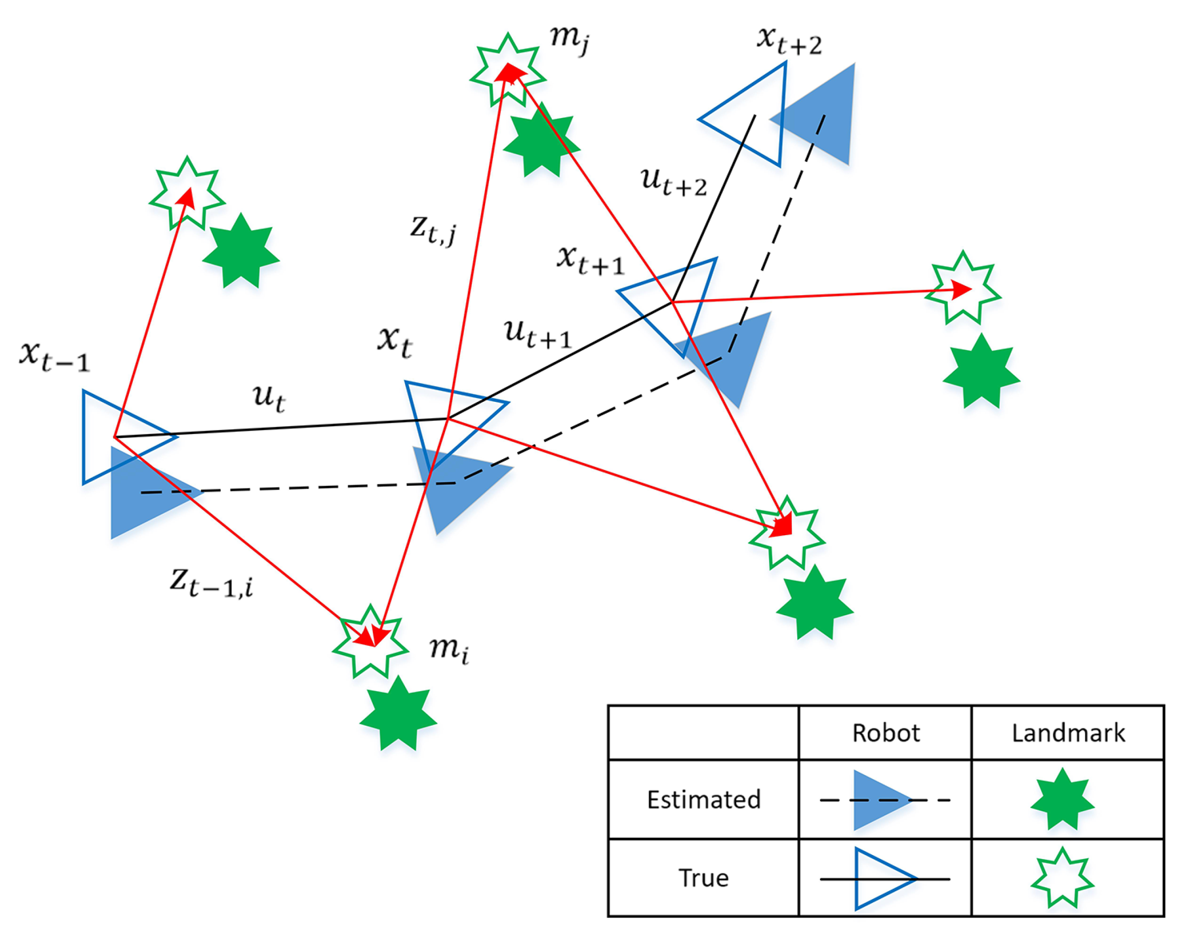
- : state vector that represents the location and orientation of the robot
- : The control input that drives the robot from state to state
- : A vector describing the position of the ith landmark
- : The observation of the ith landmark from the robot
- : The trajectory of the robot
- : The control input of the robot
- : The collection of landmark
- : The collection of landmarks’ observation
- : The correspondence variable of landmarks
2.1.1. Basic Flow of FastSLAM
- Initialisation of the particles.We initialize N particles, each of which has an initial weight .
- Retrieval.The initial step involves retrieval of a particle representing the posterior at time and the sampling of the robot’s position at time t. The position of the robot is predicted by sampling from a proposal distribution , and is denoted as for the ith particle. Normally, the proposal distribution generally adopts the probabilistic motion model .
- Importance weight.The importance weight for the ith particle represents the proportion between the target distribution and the proposal distribution mentioned above. It is defined as follows:
- Resampling.We define the effective number of particles as follows:By comparing with the threshold set in advance, it can be determined whether to perform resampling. The threshold selected here is , where N denotes the total number of particles. When , resampling is performed, in which higher weighted particles are copied and lower weighted particles are discarded.
- Measurement update.The posterior of the map feature estimation is updated based on the robot trajectory and the observation of each particle.
2.1.2. Particle Degeneracy Problem in FastSLAM
2.1.3. Adaptive GA Resampling
2.2. FastSLAM Optimised by FCPSO
2.2.1. PSO Improved by Fractional Differential
2.2.2. PSO Improved by Chaotic Optimisation
2.2.3. The Proposal of the Virtual Particle

3. Experiments
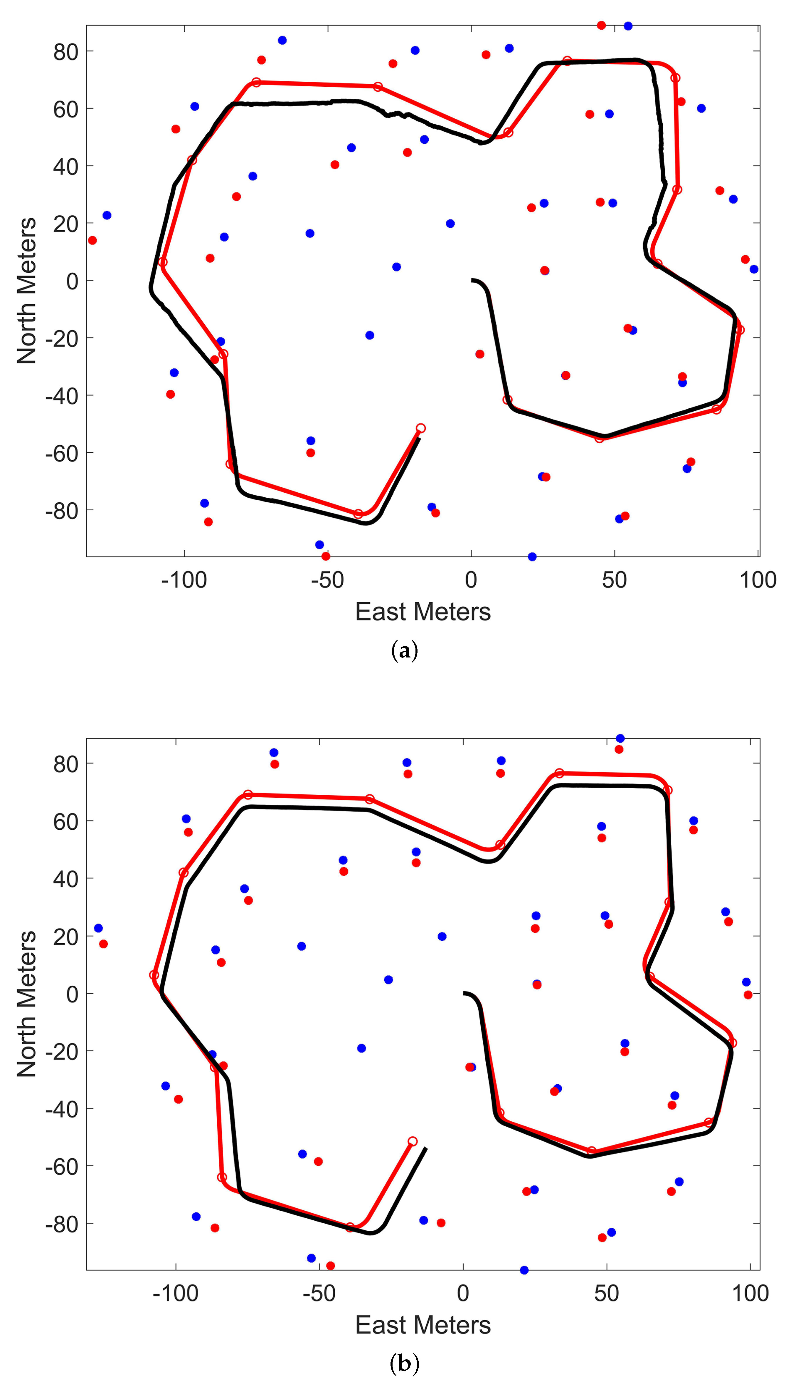
3.1. Simulation
3.1.1. Simulation Setup
3.1.2. Results and Analysis
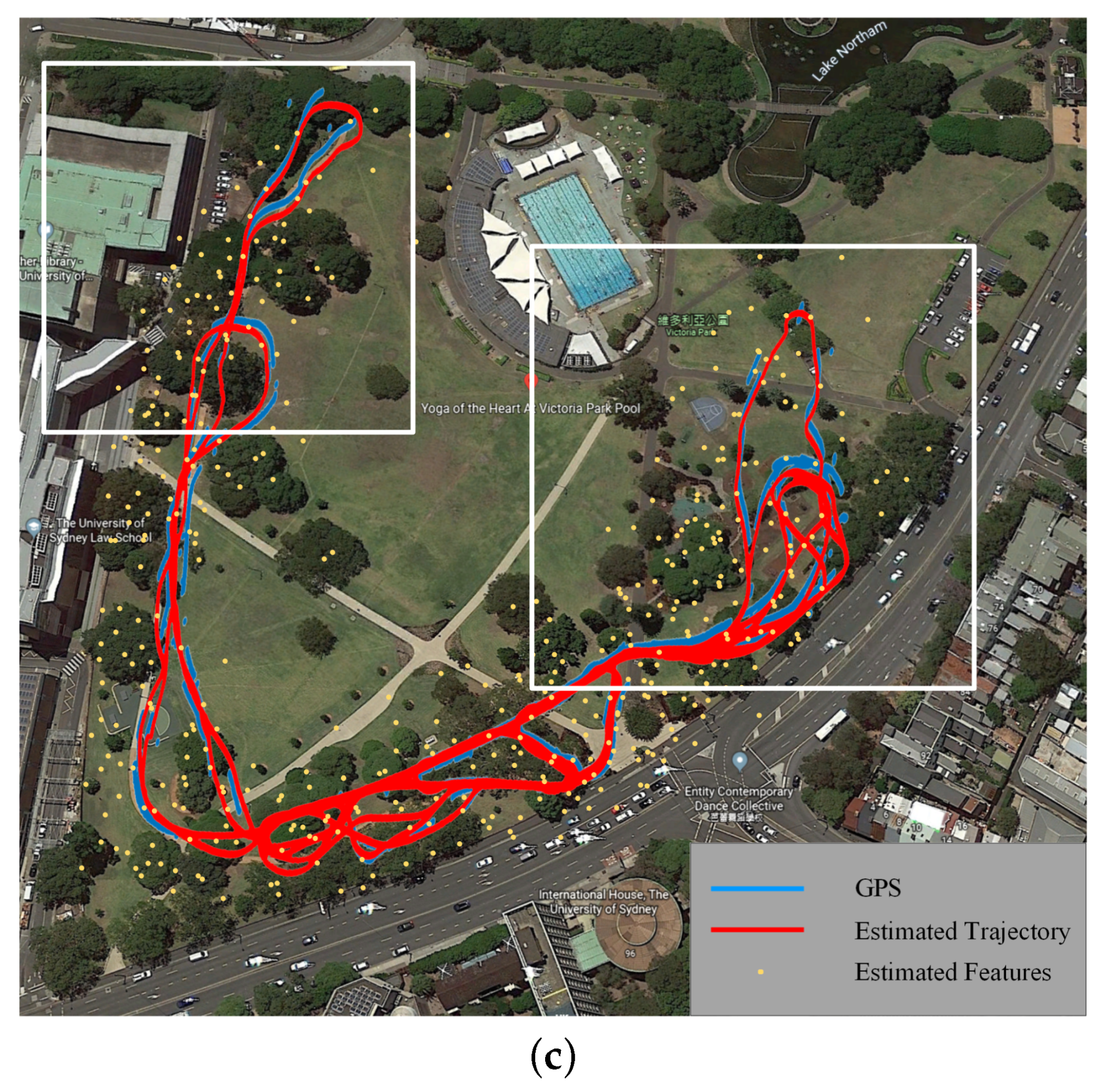
3.2. Verification Using the Victoria Park Dataset
3.3. Field Experiment
4. Conclusions
Author Contributions
Funding
Conflicts of Interest
Abbreviations
| Symbols | Implication |
| SLAM | Simultaneous localization and mapping |
| FastSLAM | Rao-Blackwellized particle filter SLA |
| EKF-SLAM | extended Kalman filter SLAM |
| AGA-Resampling | adaptive genetic algorithm resampling |
| PSO | Particle Swarm Optimisation |
| FCPSO | fractional differential and chaotic PSO |
| IFastSLAM | FastSLAM based on AGA-Resampling and optimized by FCPSO |
| the state vector describing the position and orientation of the robot | |
| the control vector, drive the robot from state to state | |
| the vector describing the position of the ith landmark | |
| the observation of the ith landmark from the vehicle at time t | |
| the importance weight of ith particle | |
| the proposal distribution of particles | |
| the effective number of particles | |
| the crossover degree of the particles | |
| the mutation probability | |
| the local optimal position of the particles of PSO | |
| the global optimal position of the swarm of PSO | |
| the velocity of ith particle at time t | |
| the position of ith particle at time t | |
| the variance of particles’ population fitness | |
| the fitness of the ith particle | |
| the average fitness of the particle swarm | |
| f | the normalization factor |
| the mean of the particle position | |
| v | the moving speed of the robot |
| G | the steering angle of the robot |
| the wheelbase of the robot | |
| the system noise at time t | |
| observation noise at time t | |
| Q | systematic noise covariance |
| R | the observation noise covariance |
Appendix A. Mathematical Proofs in the Paper
References
- Durrant-Whyte, H.; Bailey, T. Simultaneous localization and mapping: Part I. IEEE Robot. Autom. Mag. 2006, 13, 99–110. [Google Scholar] [CrossRef]
- Dissanayake, M.G.; Newman, P.; Clark, S.; Durrant-Whyte, H.F.; Csorba, M. A solution to the simultaneous localization and map building (SLAM) problem. IEEE Trans. Robot. Autom. 2001, 17, 229–241. [Google Scholar] [CrossRef]
- Maybeck, P.S. Stochastic models, estimation, and control, ser. Math. Sci. Eng. 1979, 141, 1. [Google Scholar]
- Montemerlo, M.; Thrun, S.; Koller, D.; Wegbreit, B. FastSLAM: A factored solution to the simultaneous localization and mapping problem. AAAI/IAAI 2002, 593–598. [Google Scholar] [CrossRef]
- Murphy, K.P. Bayesian map learning in dynamic environments. In Advances in Neural Information Processing Systems; The MIT Press: Denver, CO, USA, 2000; pp. 1015–1021. [Google Scholar]
- Thrun, S.; Burgard, W.; Fox, D. A real-time algorithm for mobile robot mapping with applications to multi-robot and 3D mapping. In Proceedings of the 2000 IEEE International Conference on Robotics and Automation, San Francisco, CA, USA, 24–28 April 2000; Volume 1, pp. 321–328. [Google Scholar]
- Bailey, T.; Nieto, J.; Nebot, E. Consistency of the FastSLAM algorithm. In Proceedings of the 2006 IEEE International Conference on Robotics and Automation, Orlando, FL, USA, 15–19 May 2006; pp. 424–429. [Google Scholar]
- Cugliari, M.; Martinelli, F. A FastSLAM algorithm based on the unscented filtering with adaptive selective resampling. In Field and Service Robotics; Springer: Berlin, Germany, 2008; pp. 359–368. [Google Scholar]
- Liu, D.; Duan, J.; Yu, H. FastSLAM algorithm based on adaptive fading extended Kalman filter. Syst. Eng. Electron. 2017, 38, 644–651. [Google Scholar]
- Zhang, Y.F.; Zhou, Q.X.; Zhang, J.Z.; Jiang, Y.; Wang, K. A FastSLAM algorithm based on nonlinear adaptive square root unscented Kalman filter. Math. Probl. Eng. 2017, 2017, 4197635. [Google Scholar] [CrossRef]
- Cadena, C.; Carlone, L.; Carrillo, H.; Latif, Y.; Scaramuzza, D.; Neira, J.; Reid, I.; Leonard, J.J. Past, present, and future of simultaneous localization and mapping: Toward the robust-perception age. IEEE Trans. Robot. 2016, 32, 1309–1332. [Google Scholar] [CrossRef]
- Mallik, S.; Mallik, K.; Barman, A.; Maiti, D.; Biswas, S.K.; Deb, N.K.; Basu, S. Efficiency and cost optimized design of an induction motor using genetic algorithm. IEEE Trans. Ind. Electron. 2017, 64, 9854–9863. [Google Scholar] [CrossRef]
- Li, T.; Bolic, M.; Djuric, P.M. Resampling methods for particle filtering: Classification, implementation, and strategies. IEEE Signal Process. Mag. 2015, 32, 70–86. [Google Scholar] [CrossRef]
- Lv, T.Z.; Zhao, C.X.; Zhang, H.F. An improved FastSLAM algorithm based on revised genetic resampling and SR-UPF. Int. J. Autom. Comput. 2018, 15, 325–334. [Google Scholar] [CrossRef]
- Khairuddin, A.R.; Talib, M.S.; Haron, H.; Abdullah, M.Y.C. GA-PSO-FASTSLAM: A hybrid optimization approach in improving FastSLAM performance. In International Conference on Intelligent Systems Design and Applications; Springer: Berlin, Germany, 2016; pp. 57–66. [Google Scholar]
- Kennedy, J.; Eberhart, R. Particle swarm optimization. In Proceedings of the ICNN’95—International Conference on Neural Networks, Perth, WA, Australia, 27 November–1 December 1995. [Google Scholar]
- Kwok, N.M.; Liu, D.; Dissanayake, G. Evolutionary computing based mobile robot localization. Eng. Appl. Artif. Intell. 2006, 19, 857–868. [Google Scholar] [CrossRef]
- Todor, B.; Darabos, D. Simultaneous localization and mapping with particle swarm localization. In Proceedings of the 2005 IEEE Intelligent Data Acquisition and Advanced Computing Systems: Technology and Applications, Sofia, Bulgaria, 5–7 September 2005; pp. 216–221. [Google Scholar]
- Havangi, R.; Taghirad, H.D.; Nekoui, M.A.; Teshnehlab, M. A square root unscented FastSLAM with improved proposal distribution and resampling. IEEE Trans. Ind. Electron. 2013, 61, 2334–2345. [Google Scholar] [CrossRef]
- Zhao, Y.; Wang, T.; Qin, W.; Zhang, X. Improved Rao-Blackwellised particle filter based on randomly weighted particle swarm optimization. Comput. Electr. Eng. 2018, 71, 477–484. [Google Scholar] [CrossRef]
- Lee, S.H.; Eoh, G.; Lee, B.H. Relational FastSLAM: An improved Rao-Blackwellized particle filtering framework using particle swarm characteristics. Robotica 2016, 34, 1282–1296. [Google Scholar] [CrossRef]
- Zuo, T.; Min, H.; Tang, Q.; Tao, Q. A Robot SLAM Improved by Quantum-Behaved Particles Swarm Optimization. Math. Probl. Eng. 2018, 2018. [Google Scholar] [CrossRef]
- Thrun, S. Probabilistic robotics. Commun. ACM 2002, 45, 52–57. [Google Scholar] [CrossRef]
- Kwak, N.; Lee, B.H.; Yokoi, K. Result representation of Rao-Blackwellized particle filtering for SLAM. In Proceedings of the 2008 International Conference on Control, Automation and Systems, Seoul, Korea, 14–17 October 2008; pp. 698–703. [Google Scholar]
- Yin, S.; Zhu, X. Intelligent particle filter and its application to fault detection of nonlinear system. IEEE Trans. Ind. Electron. 2015, 62, 3852–3861. [Google Scholar] [CrossRef]
- DeGroot, M.H.; Schervish, M.J. Probability and Statistics; Pearson Education: New York, NY, USA, 2012. [Google Scholar]
- Back, T. The interaction of mutation rate, selection, and self-adaptation within a genetic algorithm. In Proceedings of the 2nd Conference of Parallel Problem Solving from Nature, Brussels, Belgium, 28–30 September 1992; Elsevier Science Publishers: Amsterdam, The Netherlands, 1992. [Google Scholar]
- Zhang, X.; Zou, D.; Shen, X. A Novel Simple Particle Swarm Optimisation Algorithm for Global Optimisation. Mathematics 2018, 6, 287. [Google Scholar] [CrossRef]
- Couceiro, M.S.; Ferreira, N.F.; Machado, J.T. Application of fractional algorithms in the control of a robotic bird. Commun. Nonlinear Sci. Numer. Simul. 2010, 15, 895–910. [Google Scholar] [CrossRef]
- Pires, E.S.; Machado, J.T.; de Moura Oliveira, P.; Cunha, J.B.; Mendes, L. Particle swarm optimization with fractional-order velocity. Nonlinear Dyn. 2010, 61, 295–301. [Google Scholar] [CrossRef]
- Couceiro, M.S.; Rocha, R.P.; Ferreira, N.F.; Machado, J.T. Introducing the fractional-order Darwinian PSO. Signal Image Video Process. 2012, 6, 343–350. [Google Scholar] [CrossRef]
- Couceiro, M.S.; Ferreira, N.; Tenreiro Machado, J. Fractional order Darwinian particle swarm optimization. In Symposium on Fractional Signals and Systems; Springer International Publishing: Berlin, Germany, 2011; pp. 127–136. [Google Scholar]
- Fan, S.K.S.; Jen, C.H. An Enhanced Partial Search to Particle Swarm Optimization for Unconstrained Optimization. Mathematics 2019, 7, 357. [Google Scholar] [CrossRef]
- Pan, I.; Korre, A.; Das, S.; Durucan, S. Chaos suppression in a fractional order financial system using intelligent regrouping PSO based fractional fuzzy control policy in the presence of fractional Gaussian noise. Nonlinear Dyn. 2012, 70, 2445–2461. [Google Scholar] [CrossRef]
- Shi, Y.; Chen, G. Chaos of discrete dynamical systems in complete metric spaces. Chaos Solitons Fractals 2004, 22, 555–571. [Google Scholar] [CrossRef]
- Zhang, G.; Cheng, Y.; Yang, F.; Pan, Q. Particle filter based on PSO. In Proceedings of the 2008 International Conference on Intelligent Computation Technology and Automation (ICICTA), Hunan, China, 20–22 October 2008; Volume 1, pp. 121–124. [Google Scholar]
- Bailey, T. Source code for SLAM simulations of Tim Bailey. Available online: www.acfr.usyd.edu.au/homepages/academic/tbailey/software (accessed on 1 March 2020).
- ACFR. Victoria Park Dataset. Available online: www.acfr.us-yd.edu.au/homepages/academic/enebot/dataset.htm. (accessed on 1 March 2020).
- Nieto, J.I.; Guivant, J.E.; Nebot, E.M.; Thrun, S. Real time data association for FastSLAM. In Proceedings of the 2003 IEEE International Conference on Robotics and Automation, Taipei, Taiwan, 14–19 September 2003; Volume 1, pp. 412–418. [Google Scholar]


| Particle Number | 20 | 50 | 100 | |
|---|---|---|---|---|
| FastSLAM | Time (s) | 30.49 | 76.13 | 153.57 |
| RMSE (m) | 8.43 | 7.90 | 6.84 | |
| PSO-FastSLAM | Time (s) | 34.02 | 81.35 | 159.05 |
| RMSE (m) | 6.31 | 5.10 | 4.79 | |
| AGA-FastSLAM | Time (s) | 33.95 | 80.96 | 158.84 |
| RMSE (m) | 5.12 | 3.78 | 3.25 | |
| IFastSLAM | Time (s) | 31.17 | 78.05 | 156.98 |
| RMSE (m) | 2.85 | 2.10 | 1.71 | |
| Algorithms | Running Time (s) | RMSE (m) |
|---|---|---|
| PSO-FastSLAM | 1359.22 | 16.37 |
| AGA-FastSLAM | 1491.30 | 11.49 |
| IFastSLAM | 1406.57 | 9.15 |
| Algorithms | PSO-FastSLAM | AGA-FastSLAM | IFastSLAM |
|---|---|---|---|
| RMSE (m) | 0.27 | 0.16 | 0.09 |
© 2020 by the authors. Licensee MDPI, Basel, Switzerland. This article is an open access article distributed under the terms and conditions of the Creative Commons Attribution (CC BY) license (http://creativecommons.org/licenses/by/4.0/).
Share and Cite
Lei, X.; Feng, B.; Wang, G.; Liu, W.; Yang, Y. A Novel FastSLAM Framework Based on 2D Lidar for Autonomous Mobile Robot. Electronics 2020, 9, 695. https://doi.org/10.3390/electronics9040695
Lei X, Feng B, Wang G, Liu W, Yang Y. A Novel FastSLAM Framework Based on 2D Lidar for Autonomous Mobile Robot. Electronics. 2020; 9(4):695. https://doi.org/10.3390/electronics9040695
Chicago/Turabian StyleLei, Xu, Bin Feng, Guiping Wang, Weiyu Liu, and Yalin Yang. 2020. "A Novel FastSLAM Framework Based on 2D Lidar for Autonomous Mobile Robot" Electronics 9, no. 4: 695. https://doi.org/10.3390/electronics9040695
APA StyleLei, X., Feng, B., Wang, G., Liu, W., & Yang, Y. (2020). A Novel FastSLAM Framework Based on 2D Lidar for Autonomous Mobile Robot. Electronics, 9(4), 695. https://doi.org/10.3390/electronics9040695