Article

A 3D Shape Recognition Method Using Hybrid Deep Learning Network CNN–SVM

1
Department of IT Convergence and Application Engineering, Pukyong National University, Busan 48513, Korea
2
Department of Computer Engineering, Dong-A University, Busan 49315, Korea
*
Author to whom correspondence should be addressed.
Electronics 2020, 9(4), 649; https://doi.org/10.3390/electronics9040649
Submission received: 10 March 2020 / Revised: 13 April 2020 / Accepted: 13 April 2020 / Published: 15 April 2020
(This article belongs to the Special Issue Deep Neural Networks and Their Applications)

Abstract

:
3D shape recognition becomes necessary due to the popularity of 3D data resources. This paper aims to introduce the new method, hybrid deep learning network convolution neural network–support vector machine (CNN–SVM), for 3D recognition. The vertices of the 3D mesh are interpolated to be converted into Point Clouds; those Point Clouds are rotated for 3D data augmentation. We obtain and store the 2D projection of this 3D augmentation data in a 32 × 32 × 12 matrix, the input data of CNN–SVM. An eight-layer CNN is used as the algorithm for feature extraction, then SVM is applied for classifying feature extraction. Two big datasets, ModelNet40 and ModelNet10, of the 3D model are used for model validation. Based on our numerical experimental results, CNN–SVM is more accurate and efficient than other methods. The proposed method is 13.48% more accurate than the PointNet method in ModelNet10 and 8.5% more precise than 3D ShapeNets for ModelNet40. The proposed method works with both the 3D model in the augmented/virtual reality system and in the 3D Point Clouds, an output of the LIDAR sensor in autonomously driving cars.

1. Introduction

The 3D shapes recognition problem has been studied over a long period in the computer age with many applications in real life, such as robotics, autonomous driving, augmented/mixed reality, and so on. Many remarkable achievements in 2D object recognition have been made subsequently by the strong learning capability of a convolution neural network (CNN) and large-scale training datasets. Unlike conventional 2D images, there is a limit in the progress of 3D shape recognition [1]. The reason is that a 2D manifolds’ representation of 3D models is not similar to the representation of 2D images.
The 3D models’ representation as 2D manifolds are not similar to 2D images representation, and a standard method to store the information of 3D geometrical shapes has not been developed [2]. It seems hard to select deep learning techniques directly for 3D shape recognition. Unlike the general data formation of 2D images, the extraordinary formation of 3D shapes, such as Point Clouds and meshes as direct inputs for CNN, is one of the most challenging in CNN generalization from 3D shapes to 2D images [3]. Presentations obtained for 3D shapes have significantly affected the performance of shape recognition.
Point Clouds and mesh are two main types of 3D shapes representation. Point Clouds representation has more benefits than 3D meshes in some ways. Firstly, Point Clouds are simpler and more uniform structures for a network to learn quickly. Secondly, Point Clouds allows easy applying of the deformation due to the independence of all the points as well as no requirement in updating connected information [4]. Hence, the right choice for the classification task is directly generating 3D Point Clouds for the original 3D shape.
3D shape recognition is a base step that widely uses other tasks in intelligent electronic systems, such as 3D object tracking in intelligent robots or 3D object detection in autonomously driving cars. This paper will present the hybrid deep learning method, a combination of CNN and a Polynomial Kernel-based support vector machine (SVM) classifier, with a high accuracy in 3D shape recognition. CNN is used as the algorithm for feature extraction. The related studies are presented in section two before describing the method in section three. Then, we will compare other methods based on the numerical results. Finally, the conclusion is given.

2. Related Studies

There are two approaches: hand-crafted shape descriptors and the CNN-based method in some existing related methods for the recognition of 3D shapes.

2.1. Descriptors of Hand-Crafted Shape

Features of a hand-crafted shape consist of local and global features [5]. Global shape features, for example, viewpoint histogram [6] and shape distributions [7], proceed with the whole shape but are inappropriate for the occluded shapes recognition of messy scenes. In contrast, 3D local shape features, for example, spin image [8], rotational projection statistics (RoPS) [9], heat kernel signatures (HKS) [10], and fast point feature histogram (FPFH) [11], or 2D image features extensions, 3D SURF [12] and 2.5D SIFT [13], outperform the global features in messy scenes. Various areas, including 3D shape matching, shape recognition, and 3D shape retrieval, have applied these methods successfully with heavy dependence on human design and field experience. As a result, working on the massive 3D repositories with various objects from a variety of domains is challenging for those shape features.

2.2. CNN-Based Method

Deep learning such as CNN has outperformed conventional methods in the computer age in many problems like 3D shape recognition. The outperformance is the result of three factors: large-scale 3D datasets, obtainable deep learning structure, CNN’s training, and graphics processing units (GPU) for systems acceleration. All three factors were fairly essential for improving deep learning methods, but their challenges, as well as datasets, enable researchers to propose other studies objectively. Hence, a vast amount of studies that achieve the best recognition results gather top-quality datasets. The ModelNet dataset is adopted in most methods because it is considered to be the most appropriate challenge [14]. ModelNet, a dataset at a large scale of 3D computer-aided design (CAD) models, includes ModelNet10 and ModelNet40 subsets.
Many authors present a CNN-based method to classify the ModelNet10 dataset in their research. The ModelNet is used in the research by Garcia et al.; a PointNet is a new method for representing the input data, depending on point density occupation grids, and its integration into the CNN [15]. An insignificant accuracy percentage at 77.60% has been achieved in this study, compared with nowadays criteria, but they opened the direction for future research. The original research by Wu et al. [16] applies a convolutional deep belief network (CDBN) on the ModelNet for representation and learning of 3D shapes as possible arrangements of variables with two possible states on voxel grids at an 83.50% accuracy. Both above-mentioned methods use a voxel approach, which has a large input size and requires a lot of memory. Another method, DeepPano [17], converts from 3D shapes to panoramic scenes, applies a cylinder projection surrounding their primary axes, and uses a CNN in order to learn them. As a result, this method increases the accuracy to 88.66%. Three key views generate the depth panoramic. This panoramic designs three branches of the CNN system, so-called 3V-DepthPano CNN [18]. This V-DepthPano CNN adopts a three-branch CNN for accumulating the 3D shape depth panoramic data into a smaller 3D shape descriptor for the classification of the 3D shape. This model obtains the highest accuracy at 89.83%. DeepPano and 3V-DepthPano use a view-based approach. Both DeepPano and our method use one view for each 3D shape, compared with three views in the 3V-DepthPano. The idea of the 3V-DepthPano is mainly based on multi-view convolutional neural networks (MVCNN) [19], but it uses three views instead of 12 views and 80 views in MVCNN. The linear interpolation algorithm allows our method to work with only one view for each 3D shape to handle the drawbacks of multi-view methods. The high computational and memory cost is one of the main limitations of multi-view methods. This drawback causes a big challenge on the constraint resource memory in practical applications, such as an intelligent robot. The second drawback of multi-view methods is inconsistent recognition accuracy due to incomplete views cases. The full-view assumption of the multi-view methods, which requires data from all views to be observed, seems to be violated in practical applications. For example, human error causes data loss from certain views, which may produce multi-view data with incomplete views [20].
This article represents the new recognition method that captures more spatial information of a 3D shape for a view-based approach, in comparison with the previous studies. Table 1 compares previous methods with the proposed method in which all use the view-based approach. DeepPano may lead to missing information at the top and the bottom of a 3D shape because this method uses only a single view. The 3V-DepthPano method applies three views, such as front view, top view, and left view, to obtain 2D views. Three views in the method are designed to represent the 3D shape structure. The depth panorama images, which are obtained by cylindrical projection in the three-view directions, are also included in this representation. The depth panorama images play as part of the input of the parallel network for training. The drawback of 3V-DepthPano is that it consumes the most memory for each input data and uses parallel CNN. In the proposed method, we construct the new 3D shape representation that allows the single 2D projection to avoid the loss of spatial information without a parallel CNN network. For example, the four wheels of the 3D shape car use a single 2D projection without building a panoramic view while two methods, DeepPano and 3V-DepthPano, could not do that task.
The paper proposes a method to interpolate the original vertices of a 3D shape with a linear interpolation algorithm to create a new 3D Point Clouds dataset. Our derivation is not known in the literature to the best of our knowledge. The interpolation algorithm creates a good 2D representation for 3D shapes, which surpass the challenges in lost spatial information. Moreover, we design appropriate deep learning architecture to combine with the 2D projection of the interpolation 3D Point Clouds that minimize the input data size of 2D CNN and improve the recognition accuracy. The interpolation algorithm makes information for 2D projection more spatial. This allows us to build an effective recognition method with an uncomplicated CNN structure, which could not build when applying the view-based approach directly to the original 3D shape dataset.
While all the four methods (PointNet, 3D ShapeNets, DeepPano, 3V-DepthPano) use CNN for both classification and feature extraction, we will apply CNN for feature extraction and SVM for the classification in the paper. A brief description of the SVM will be given below. Our goal is to maximize the margin and reduce the classification error between two classes of data y i ∈ {+1, −1} for searching the optimum hyperplane in binary classification problems with linear separability (Figure 1).
SVM with the kernel function makes a transformation of the original data space to a higher dimensional one [21], which handles the challenge of data divergence as well as nonlinear separability in the classification process. We aim to obtain the transformed data in a higher dimension with easy separability. Nanda et al. [22] presents the numerical results with the highest classification accuracy using the SVM algorithm with the polynomial kernel, so the polynomial kernel is chosen in our paper.

3. Methodology

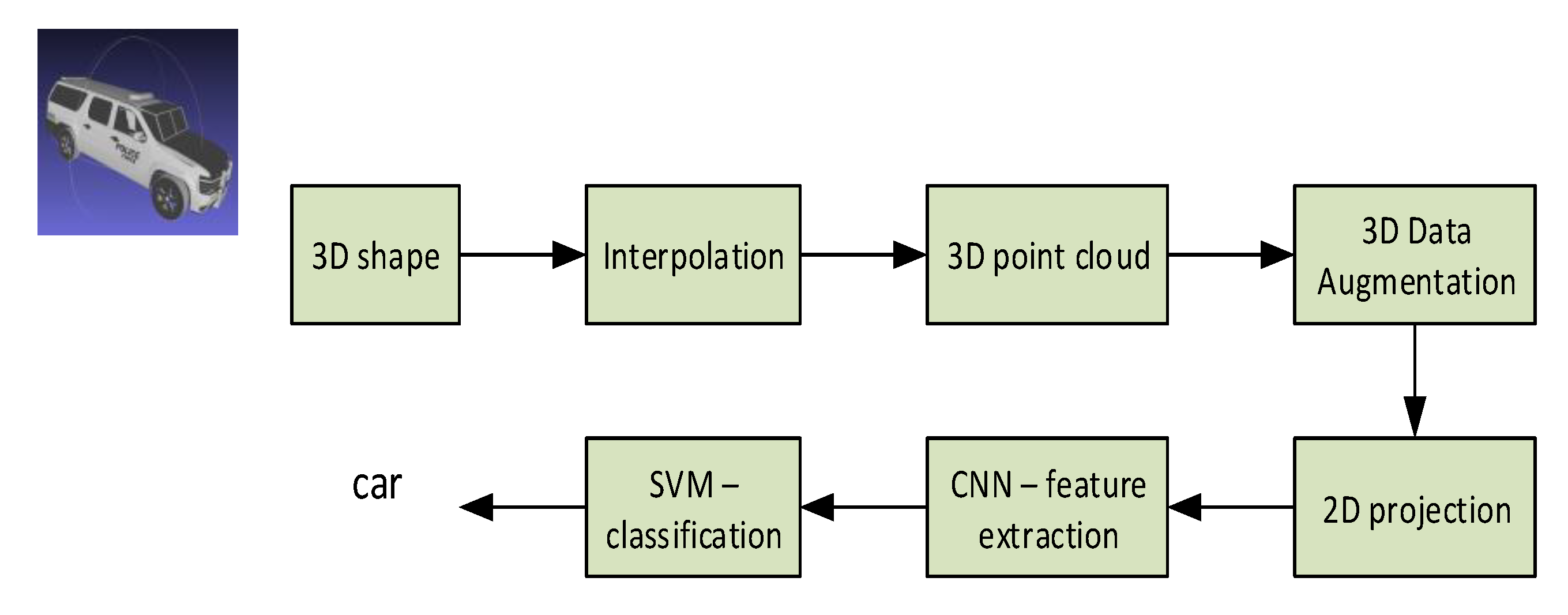
As shown in Figure 2, the original 3D shape is first used for generating the 3D Point Clouds; these Point Clouds are rotated for the data augmentation and create the 2D projection. We use the hybrid deep learning network convolution neural network–support vector machine (CNN–SVM) for feature extraction and classification at the final step. Our method will be fully explained in the next section.

3.1. The Creation of 3D Point Clouds Data

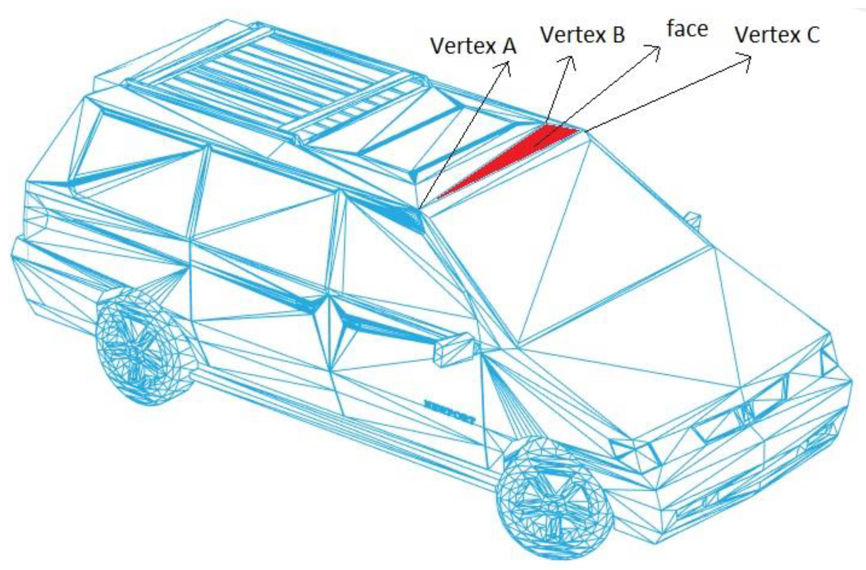
We interpolate all vertices of the original 3D shape to produce the 3D Point Clouds. The 3D shape, including the faces and vertices, have file the formats STL, OBJ, and OFF. These file formats use the triangular faces with three vertices for each face. Figure 3 shows the OFF file with only 41,285 vertices (without 22,034 faces).
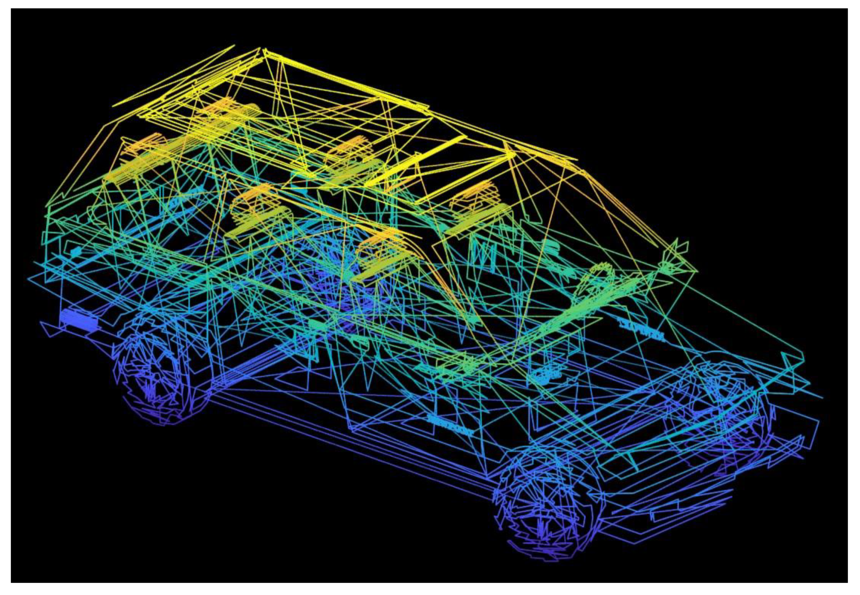
We will interpolate 510 points P i , 1 , P i , 2 , , P i , 510 between two adjacent vertices V i ( x i , y i , z i ) and V i + 1 ( x i + 1 , y i + 1 , z i + 1 ) (i = 1,2, …, M − 1) among M vertices V 1 ,   V 2 ,     ,   V M of the 3D shape using Equation (1). This interpolation technique will create 512 equally spaced points in the interval [ V i ( x i , y i , z i ) ,   V i + 1 ( x i + 1 , y i + 1 , z i + 1 ) ] .
P i , j = ( 1 j 511 ) V i + j 511 V i + 1 ;       j = 1 : 510 .
Figure 4 shows the interpolation results of the original 3D shape. We can see that Point Clouds explore the interior designs such as chairs, the steering wheels, and the opposite wheels beside the reservation of the 3D shape boundary.

3.2. D Point Clouds Data Augmentation

As we have known, an insufficient amount of training data or unbalanced datasets are challenges in deep learning. Data augmentation, such as rotating, cropping, zooming, and histogram-based methods in conventional image transformation, are one method for solving these problems in 2D images classification [23]. It is reasonable for us to extend to 3D from these 2D methods by choosing a rotation approach for 3D Point Clouds. Figure 5 shows the original Point Clouds and Point Clouds after rotating by 90, 180, and 270 degrees, respectively.
We will normalize the 3D point by dividing all current elements in Point Clouds, P C 1   (a nx3 matrix with the number of points at n), by the maximum coordinate values of the P C 1 before the rotation. As a result, three coordinate values of Point Clouds will be inside the unit cubic (−1 < x < 1, −1 < y < 1, −1 < z < 1).
P C 1 = P C 1 max ( max ( P C 1 ) ) .
Rodrigues' rotation formula [24] is adapted to rotate the 3D Point Clouds, as given by Equation (3).
P C 1 , R = R m a t r i x P C 1 ,
R m a t r i x = I + ( s i n ( R o t A n g l e ) ) H + ( 1 c o s ( R o t A n g l e ) ) H 2 ,
H = ( 0   h 3       h 2 h 3           0             h 1 h 2         h 1         0         ) ,
where R m a t r i x is the rotation matrix; P C 1 is the original Point Clouds; P C 1 , R is a rotated Point Clouds; RotAngle is the angle of the rotation in the degree; H is the skew-symmetric; h = (   h 1 , h 2 ,   h 3 ) = ( 1 0 0 ); the rotation axis is Ox.
We rotate to obtain three more 3D shapes and four 3D shapes in total for each 3D shape in the dataset. Furthermore, we obtain four projections in total with a 32 × 32 × 3 size for each projection from each 2D projection of each 3D shape. The concatenation of these four projections along the third dimension produces a 32 × 32 × 12 matrix A as the input data of CNN.

3.3. The Architecture of CNN–SVM

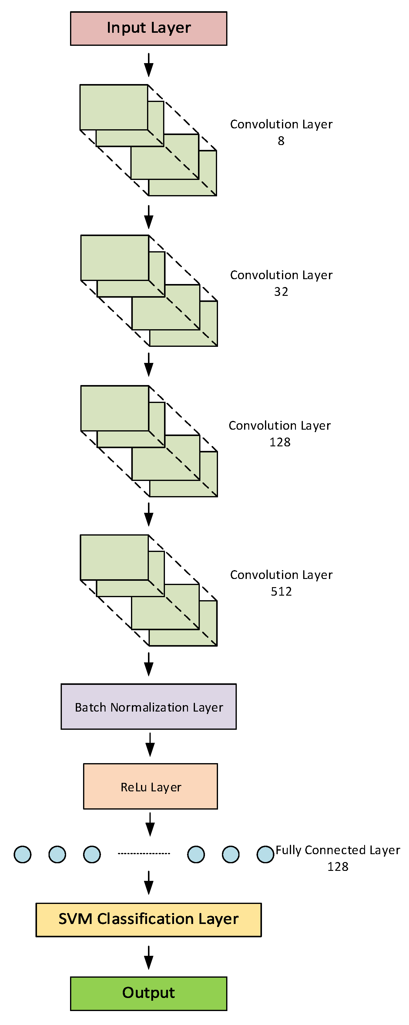
The CNN–SVM architecture in the proposed method consists of an input layer, followed by four convolutional layers with 8, 32, 128, and 512 filters, respectively (see Figure 6). We set values 1 for the padding for all convolutional layers, and the stride equals 1. Then, the fourth convolution layer is followed respectively by batch normalization and the rectified linear unit (ReLU) layer, and fully connected layer. Finally, CNN–SVM uses the SVM for the classification of the feature extract. There are some reasons for using the batch normalization layer in our network. Batch normalization not only speeds the training of neural networks but also allows to reduce overfitting by regularity, use the higher learning rates with fewer parameter initialization. A network’s activations over a mini-batch are normalized by batch normalization. More specifically, these activations subtract their means, all divided by their standard deviations. Hence, batch normalization is used to increase convergence speeds and to prevent model divergence [25].
The first convolution layer, which inputs matrix A to apply a padding 1, and 1 × 1 stride-convolution function, produces eight feature maps traveling to the second convolution layer. The second, third, and fourth convolution layers produce 32, 128, and 512 feature maps with the dimensions of 34 × 34, 35 × 35, and 36 × 36, respectively. The output of the fourth convolution layer with a feature vector at size 512 is taken by the batch normalization layer. The output of the batch normalization layer moves to the ReLU layer, then to the fully connected layer.
The softmax activation function is employed in most of the deep learning models to predict and minimize cross-entropy loss in classification tasks. Tang et al. [26] uses linear SVM instead of softmax for classification accuracy improvement on datasets, such as MNIST, CIFAR-10, and the ICML 2013. Softmax will be replaced by polynomial SVM in this paper. For each testing 3D shape, the SVM classification layer takes 128 feature vectors from the fully connected layer output and decides the corresponding class among L classes (L = 10 or 40).
The original problem of the SVM algorithm is binary classification, as seen in Figure 1 (linear separable case). Suppose that we have a training data set ( x 1 , y 1 ), ( x 2 , y 2 ), …, ( x N , y N ), where x i is the i-th training data and y i is the corresponding label. The equation of the hyperplane is w T x + b = 0 . The nearest red point to the hyperplane satisfies w T x + b = 1 . If the new data point satisfies w T x + b > 1 , it will belong to the red class (class 1), and vice versa.
SVM’s problem in binary classification is to find w and b so that the margin is maximized. The SVM problem is defined as a quadratic optimization problem, shown in formula six.
argmin w , b 1 2 w 2 2   s u c h   t h a t   y i ( w T x i + b ) 1 ,   i = 1 , 2 , , N .  
The dual form is defined as
  argmax α i = 1 N α i 1 2 i = 1 N j = 1 N α i α j y i y j x i T x j   s u c h   t h a t   i = 1 N α i y i = 0 , α i 0   i = 1 , 2 , , N ,   where   α i   are   Lagrange   multipliers .  
The data is normally non-linear for multi-classification, and SVM transforms non-linear data to linear by using mapping function, namely, . This mapping transforms original data to a higher dimension space that is linearly separable. The term x i T x j in Equation (7) is replaced by ( x i T ) ( x j ) in the multi-classification problem. Practically, it is unnecessary to calculate ( x ) for all data points, so we need to calculate the only ( x i T ) ( x j ) for any two data points. From this point, the concept kernel, K ( x i , x j ) = ( x i T ) ( x j ) , is introduced. The polynomial kernel in this study is defined in the following equation.
K ( x i , x j ) = ( 1 + x i T x j ) D ,   D   is   degree   of   polynomial   kernel .
This study uses a one-versus-one approach for multi-classification SVM, which constructs L ( L 1 ) 2 pairwise binary classifications SVM (L is the number of classes). The most frequent predicted class, which wins most among these pairwise binary classifications for one-versus-one multiclass SVM, is defined as the final prediction for a test point. Let consider an example with L = 4, and the four classes, namely, A, B, C, and D. Multi-classification SVM will use six binary classifications SVM to predict the class of a test point. The first binary classification will determine whether a test point belongs to class A or B. Similarly, the remaining five binary classifications will predict whether a test point belongs to class A or class C, class A or class D, class B or class C, class B or class D, and class C or class D. Suppose that the results for six binary classification SVM are B, A, D, B, B, D, then the final prediction will be class B with the highest frequency (frequency is 3).

4. Experimental Results

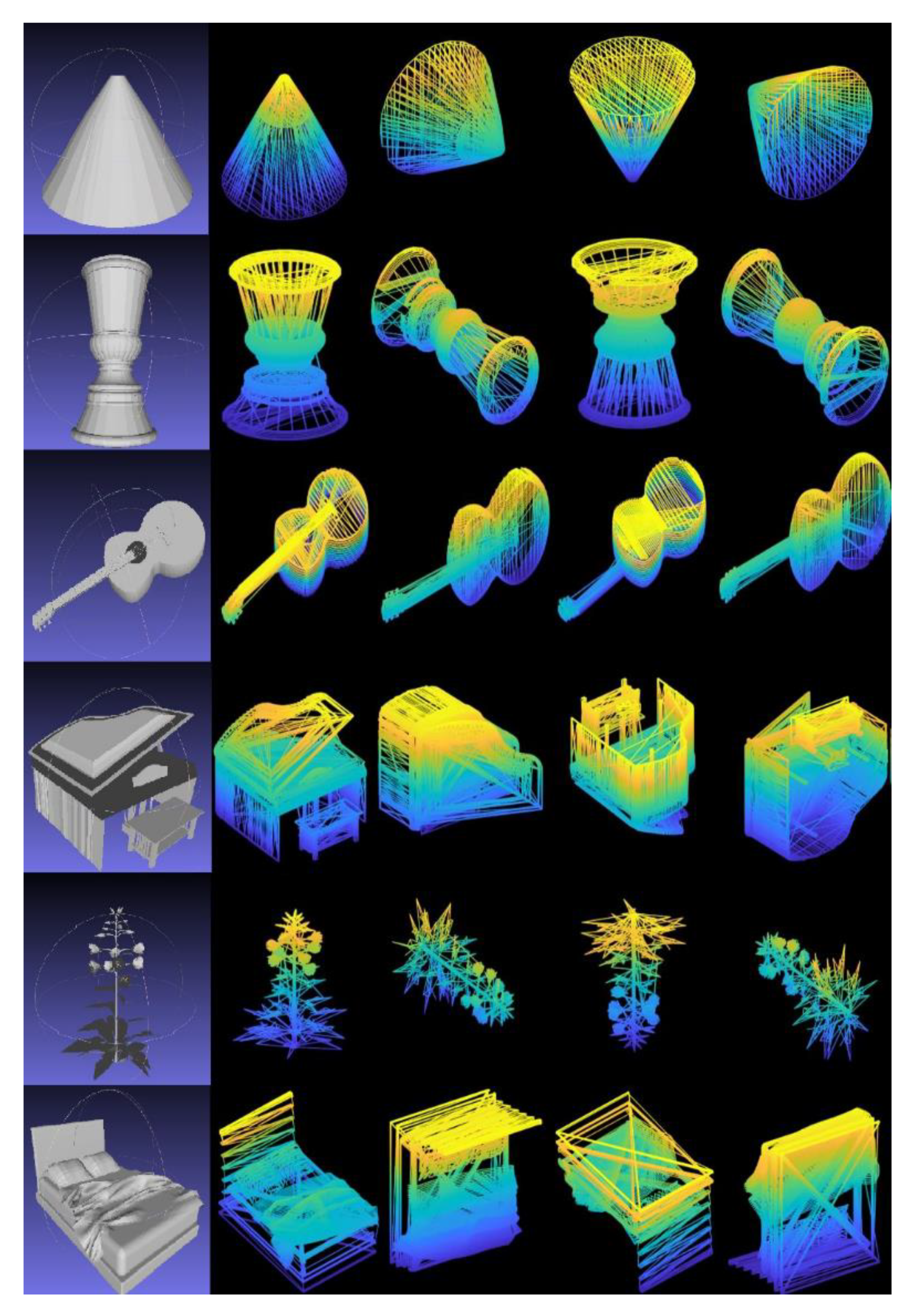
Our experiments will work on the ModelNet dataset, including ModelNet10 and ModelNet40 [16]. The original ModelNet dataset can be downloaded from the website in the Supplementary Materials. The 3D CAD of ModelNet10 has ten categories with 3991 training and 908 testing models, comparing forty categories with 9843 training and 2468 testing models from the 3D CAD of ModelNet40. OFF is a 3D-triangle mesh format of each CAD model of ModelNet. The number of models of a specific class for the ModelNet40 is shown in Table 2. In case that the model has less than 128,000 vertices, all CAD models in the original dataset are interpolated. If the model has more than 128,000 vertices, the original model is still kept without interpolation due to the differences in the number of model vertices in the same class. For example, the airplane class has the maximum vertices at 2,286,376 and the minimum at 1107 before interpolation, so the ratio is 2,286,376/1107 = 2065.38. After the interpolation process, we have 1106 × (510) + 1107 = 565,167 total points, and the ratio is 2,286,376/565,167 = 4.05. Figure 7 shows the 2D projections from the 3D rotation on 3D Point Clouds of random models in the ModelNet40 dataset.
We implemented all experiments on the computer I7 7700, 32GB memory, 1080Ti GPU, windows 10, MATALB (9.7 (R2019b), Natick, MA, USA). The network is trained by choosing Adam optimization Algorithm at the momentum 0.9, at the mini-batch size 16, and with the initial learning rate 0.000001. The polynomial kernel is used in SVM with the hyperparameters at degree 2, gamma 0.001, and cost 1. The training time for ModelNet10 and ModelNet40 is 4.5 hours and 15.5 hours, respectively. Figure 8 shows that our method is more accurate than others with precision at 91.08% and 85.82% for ModelNet10 and ModelNet40, respectively. The PointNet and 3D ShapeNets have the lowest precision levels, with 77.60% on the evaluation of only the ModelNet10 dataset for the PointNet, and with 83.54% on ModelNet10 and 77.32% on ModelNet40 for the 3D ShapeNets.
The PointNet and 3D ShapeNets work with the voxel, which has a 30 × 30 × 30 minimum size for each 3D shape. In Matlab, the default class double requires eight bytes per element of memory for storage. Hence a 3D matrix of size 30 by 30 by 30 takes 0.206 Mb of memory. In contrast, the proposed method describes each 3D shape by a 32 ×32 × 12 matrix, and thereby takes 0.094 Mb of memory (half the size of the voxel approach). DeepPano, PanoView, and 3V-DepthPano belong to the group of the view-based method. In these three methods, a cylindrical surface whose central axis concurs the principal axis of the model surrounds the 3D model for building a panoramic view. DeepPano and PanoView construct a panoramic view from one key view, while 3V-DepthPano uses three different panoramic views from three key views. 3V-DepthPano gains the highest accuracy but requires the largest input data size at 227 by 227, which consumes 0.393 Mb of memory, is four times the memory of the proposed method. Moreover, 3V-DepthPano is the only method which uses parallel CNN structure with three-branch CNN, causing the high complexity of deep learning network. The proposed method could get better accuracy without constructing a cylindrical surface and panoramic view because it directly captures a single 2D projection of 3D interpolation Point Clouds based on the linear interpolation algorithm. In addition, the proposed method uses single CNN instead of multi-branch CNN. Furthermore, our method contains more spatial information with a single 2D projection, such as the opposite side of the cone and Flower Pot, as seen in Figure 7.
There is at least one parameter in the pooling layer and no parameters in batch normalization and the ReLU layer for all other methods. There are five convolution layers in the 3V-DepthPano which use the Alexnet model [27]. Both Panoramic View [3] and DeepPano use four convolution Blocks with one convolution layer for each block, followed by a max-pooling layer, compared with four convolution layers in our method. The number of parameters in the fully-connected layers is not compared because there is no information on the number of feature vectors of this layer in the DeepPano method in [17]. The first and second layers of the Panoramic View used 512 and 1024 feature vectors, respectively, while both layers of the 3V DepthPano method had 4096 vectors. Unlike these methods, one fully connected layer with 128 feature vectors will be used. Our method used fewer parameters at 3400 in total for all convolution layers than their methods with 18,112 for DeepPano, 15,088 for Panoramic View, and 28,608 for 3V-DepthPano (see Table 3). Therefore, our method is more efficient because it reduces model parameters, and as a result, diminishes the computational cost. Panoramic View and DeepPano choose parameters approximately equal and have similar accuracy at 82.54% and at 82.47%, respectively, for ModeleNet40. Panoramic View made a 1.14% accuracy increment in the classification task on ModelNet10, compared with DeepPano, and has the same accuracy with 3V-DepthPano. Because 3V-DepthPano has twice as many parameters as Panoramic View, it shows a 6.49% higher accuracy in the ModelNet40 classification.
Our method is more accurate on ModelNet40 than on other methods, except 3V-DepthPano. The main reason is that the number of parameters in 3V-DepthPano, namely, 28,608, is 8.41 times the corresponding parameters in our method, and the 3V-DepthPano used the highest input at a 227 x 227 size. Figure 9 shows a confusion plot for ModelNet10 and ModelNet40. The most misclassified percentages are 25% for the Flower Pot class and 40% for the Cup class. Flower Pots are misclassified as Plants at 50%, and Cups are predicted as vases at 20%. The data representation helps our methods to obtain the highest accuracy in the ModelNet10 dataset, as shown in Figure 8. DeepPano used only one view, while 3V-DepthPano had complete information in three views. This is one of the reasons why 3V-DepthPano outperforms DeepPano. The information of the 3D shape in our method is explored externally and internally; for example, the interior designs of the car class is stored. Therefore, the proposed method achieved higher accuracy.
The proposed method performs best, except that the recognition for the cup object class still has a low accuracy. The imbalance between classes in the dataset in the study may affect the results. The rate of success in object recognition is opposite with an increase and a decrease in a higher and a lower number of training samples, respectively. Oversampling techniques could handle the class imbalance and reduce uncertainties in the minority classes because it adds an amount to the training data for these classes. The direction for future research is that we design new oversampling techniques to eliminate the imbalance between classes.
The object recognition method in this study can work with an intelligent robot using the Microsoft Kinect sensor. At the initial step, the robot could not recognize various objects such as a person, cup, bottle, and desk in the scene. Next step, the robot queries the feature vectors of the offline dataset; these feature vectors are extracted by using the proposed method. Then, the robot assigns the labels for the extracted features from the constructed 3D object. This 3D object is captured by the Kinect sensor. Finally, the robot can fully recognize objects.

5. Conclusions

In this paper, we present good choices of 3D data representation, 3D data interpolation, and the hybrid structure CNN–SVM on a big dataset. Our novel approach enhances the limit of evaluation on only a small number of the model of 3D shape recognition in the past. Based on our numerical results, our method is more accurate and efficient than five other methods (see Figure 8). The proposed method is 13.48% and 8.5% more accurate than the PointNet in ModelNet10 and the 3D ShapeNets in ModelNet40, respectively. Recognition is an essential task in various computer vision applications, such as human–machine interaction. Our methods flexibly adapted in a 3D point cloud system like the LIDAR sensor, and thus work well with two types: 3D shape mesh and Point Clouds. The LIDAR sensor could produce 3D Point Clouds of one object with hundreds of millions of points. In contrast, our method can reuse the CAD model dataset to create the 3D Point Clouds with fewer points. We aim to integrate the program into problems in real life, such as self-driving cars or AR/VR software for future research and development.

Supplementary Materials

The original ModelNet dataset is available online at https://modelnet.cs.princeton.edu/.

Author Contributions

Conceptualization, L.H.; funding acquisition, K.-R.K.; investigation, L.H.; methodology, L.H.; project administration, K.-R.K.; software, L.H.; supervision, K.-R.K.; validation, K.-R.K.; writing—original draft, L.H.; writing—review & editing, L.H., S.-H.L., and K.-R.K. All authors have read and agreed to the published version of the manuscript.

Funding

This research received no external funding.

Acknowledgments

This research was supported by the MSIT (Ministry of Science and ICT), Korea, under the ICT Consilience Creative program (IITP-2020-2016-0-00318) supervised by the IITP (Institute for Information & communications Technology Promotion).

Conflicts of Interest

The authors declare no conflict of interest.

References

  1. Zaki, H.; Shafait, F.; Mian, A. Modeling 2D appearance evolution for 3D object categorization. In Proceedings of the 2016 International Conference on Digital Image Computing: Techniques and Applications (DICTA), Gold Coast, Australia, 30 November–2 December 2016; pp. 1–8. [Google Scholar] [CrossRef]
  2. Bu, S.; Wang, L.; Han, P.; Liu, Z.; Li, K. 3D shape recognition and retrieval based on multi-modality deep learning. Neurocomputing 2017, 259, 183–193. [Google Scholar] [CrossRef]
  3. Zheng, Q.; Sun, J.; Zhang, L.; Chen, W.; Fan, H. An improved 3D shape recognition method based on panoramic view. Math. Probl. Eng. 2018, 2018, 11. [Google Scholar] [CrossRef]
  4. Xia, Y.; Wang, C.; Xu, Y.; Zang, Y.; Liu, W.; Li, J.; Stilla, U. RealPoint3D: Generating 3D point clouds from a single image of complex scenarios. Remote Sens. 2019, 11, 2644. [Google Scholar] [CrossRef] [Green Version]
  5. Zhi, S.; Liu, Y.; Li, X.; Guo, Y. LightNet: A lightweight 3D convolutional neural network for real-time 3D object recognition. In Proceedings of the 2017 Workshop on 3D Object Retrieval (3Dor17), Lyon, France, 23–24 April 2017; pp. 9–16. [Google Scholar] [CrossRef]
  6. Rusu, R.; Bradski, G.; Thibaux, R.; HsuRetrievalb, J. Fast 3D recognition and pose using the viewpoint feature histogram. In Proceedings of the 2010 IEEE/RSJ International Conference on Intelligent Robots and Systems, Taipei, Taiwan, 18–22 October 2010; pp. 2155–2162. [Google Scholar] [CrossRef]
  7. Osada, R.; Funkhouser, T.; Chazelle, B.; Dobkin, D. Shape distributions. ACM Trans. Graph. 2002, 21, 807–832. [Google Scholar] [CrossRef]
  8. Johnson, A.; Herbert, M. Surface matching for object recognition in complex 3-dimensional scenes. Image Vision Comput. 1998, 16, 635–651. [Google Scholar] [CrossRef]
  9. Guo, Y.; Sohel, F.; Bennamoun, M.; Lu, M.; Wan, J. Rotational projection statistics for 3D local surface description and object recognition. Int. J. Comput. Vis. 2013, 105, 63–68. [Google Scholar] [CrossRef] [Green Version]
  10. Sun, J.; Ovsjanikov, M.; Guibas, L. A concise and provably informative multi-scale signature based on heat diffusion. Comput. Graph. Forum 2009, 28, 1383–1392. [Google Scholar] [CrossRef]
  11. Rusu, R.; Blodow, N.; Beetz, M. Fast point feature histograms (FPFH) for 3D registration. In Proceedings of the 2009 IEEE International Conference on Robotics and Automation, Kobe, Japan, 12–17 May 2009; pp. 1848–1853. [Google Scholar] [CrossRef]
  12. Knopp, J.; Prasad, M.; Willems, G.; Timofte, R.; Gool, L. Hough transform and 3D SURF for robust three dimensional classification. In Proceedings of the 11th European Conference on Computer Vision (ECCV 2010), Heraklion, Crete, Greece, 5–11 September 2010; pp. 589–602. [Google Scholar] [CrossRef]
  13. Lo, T.; Siebert, J. Local feature extraction and matching on range images: 2.5D SIFT. Comput. Vis. Image Und. 2009, 113, 1235–1250. [Google Scholar] [CrossRef]
  14. Gomez-Donoso, F.; Garcia-Garcia, A.; Garcia-Rodriguez, J.; Orts-Escolano, S.; Cazorla, M. LonchaNet: A sliced-based CNN architecture for real-time 3D object recognition. In Proceedings of the 2017 International Joint Conference on Neural Networks (IJCNN), Anchorage, AK, USA, 14–19 May 2017; pp. 412–418. [Google Scholar] [CrossRef]
  15. Garcia, A.; Donoso, F.; Rodriguez, J.; Escolano, S.; Cazorla, M.; Lopez, J. PointNet: A 3D convolutional neural network for real-time object class recognition. In Proceedings of the 2016 International Joint Conference on Neural Networks (IJCNN 2016), Vancouver, BC, Canada, 24–29 July 2016; pp. 1578–1584. [Google Scholar] [CrossRef]
  16. Wu, Z.; Song, S.; Khosla, A.; Yu, F.; Zhang, L.; Tang, X.; Xiao, J. 3D ShapeNets: A deep representation for volumetric shapes. In Proceedings of the 2015 IEEE Conference on Computer Vision and Pattern Recognition (CVPR ’15), Boston, MA, USA, 7–12 June 2015; pp. 1912–1920. [Google Scholar] [CrossRef] [Green Version]
  17. Shi, B.; Bai, S.; Zhou, Z.; Xiang, B. DeepPano: Deep panoramic representation for 3-D shape recognition. IEEE Signal Process. Lett. 2015, 22, 2339–2343. [Google Scholar] [CrossRef]
  18. Yin, J.; Huang, N.; Tang, J.; Fang, M. Recognition of 3D shapes based on 3V-DepthPano CNN. Math. Probl. Eng. 2020, 2020, 11. [Google Scholar] [CrossRef]
  19. Su, H.; Maji, S.; Kalogerakis, E.; Learned-Miller, E. Multi-view convolutional neural networks for 3d shape recognition. In Proceedings of the IEEE international conference on computer vision (ICCV), Santiago, Chile, 7–13 December 2015; pp. 945–953. [Google Scholar] [CrossRef] [Green Version]
  20. Zhao, J.; Xie, X.; Xu, X.; Sun, S. Multi-view learning overview: Recent progress and new challenges. Inf. Fusion. 2017, 38, 43–54. [Google Scholar] [CrossRef]
  21. Valiollahzadeh, S.; Sayadiyan, A.; Nazari, M. Feature selection by KDDA for SVM-based multiview face recognition. arXiv 2008, arXiv:0812.2574. [Google Scholar]
  22. Nanda, M.; Seminar, K.; Nandika, D.; Maddu, A. A Comparison Study of Kernel Functions in the Support Vector Machine and Its Application for Termite Detection. Information 2018, 9, 5. [Google Scholar] [CrossRef] [Green Version]
  23. Mikołajczyk, A.; Grochowski, M. Data augmentation for improving deep learning in image classification problem. In Proceedings of the 2018 International Interdisciplinary PhD Workshop (IIPhDW), Swinoujście, Poland, 9–12 May 2018; pp. 117–122. [Google Scholar] [CrossRef]
  24. Orientation, Rotation, Velocity and Acceleration. Available online: https://www.sedris.org/wg8home/Documents/WG80485.pdf (accessed on 28 February 2020).
  25. Schilling, F. The Effect of Batch Normalization on Deep Convolutional Neural Networks; DiVA Publisher: Uppsala, Sweden, 2016. [Google Scholar]
  26. Tang, Y. Deep Learning using Linear Support Vector Machines. arXiv 2013, arXiv:1306.0239. [Google Scholar]
  27. Krizhevsky, A.; Sutskever, I.; Hinton, G. ImageNet Classification with Deep Convolutional Neural Networks. In Proceedings of the 2012 Annual Conference on Neural Information Processing Systems (NIPS), Lake Tahoe, NV, USA, 3–8 December 2012; pp. 1106–1114. [Google Scholar] [CrossRef]
Figure 1. The support vector machine (SVM) with the linear separable case.
Electronics 09 00649 g001
Figure 2. The proposed method.
Electronics 09 00649 g002
Figure 3. A total of 41,285 vertices of one 3D shape.
Electronics 09 00649 g003
Figure 4. The interpolation Point Clouds.
Electronics 09 00649 g004
Figure 5. The original Point Clouds on the top left and three Point Clouds rotated.
Electronics 09 00649 g005
Figure 6. The hybrid deep learning architecture of the proposed method.
Electronics 09 00649 g006
Figure 7. The Random models and four 2D projections of Point Clouds from the dataset: ModelNet40.
Electronics 09 00649 g007
Figure 8. The comparison between the proposed method and other methods, PointNet evaluates only ModelNet10.
Electronics 09 00649 g008
Figure 9. The confusion matrix for datasets: Modelnet10 (top) and ModelNet40 (bottom).
Electronics 09 00649 g009
Table 1. A comparative overview among methods.
MethodsDeepPano3V-DepthPanoProposed Method
ApproachView-basedView-basedView-based
Transform 3D shapeNoNoInterpolate vertices
Type of 2D viewsPanoramic viewsPanoramic viewsSingle 2D projection
Multi-CNN structureSingle CNNThree-branch CNNSingle CNN
Table 2. Classes distribution of ModelNet40.
Class NameTotalClass NameTotalClass NameTotalClass NameTotal
airplane726cup99laptop169sofa780
bathtub156curtain158mantel384stairs144
bed615desk286monitor565stool110
bench193door129night_stand286table492
bookshelf672dresser286person108tent183
bottle435Plower_pot169piano331toilet444
bowl84Glass_box271plant340tv_stand367
car297guitar255radio124vase575
chair989keyboard165range_hood215wardrobe107
cone187lamp144sink148xbox123
Table 3. The total parameters for all convolution layers of various methods.
LayersDeepPanoParametersPanoViewParameters
Input160 × 640108 × 360
Conv1(5, 96)2496(1, 64)128
Conv2(5, 256)6656(2, 80)400
Conv3(3, 384)3840(4, 160)2720
Conv4(3, 512)5120(6, 320)11,840
FC1N.AvailableN.Available512N.Available
FC2N.AvailableN.Available1024N.Available
Total-18,112-15,088
Layers3V-DepthPanoParametersOur MethodParameters
Input227 × 227032 × 32 × 120
Conv1(11, 96)11,712(2, 8)40
Conv2(5, 256)6656(2, 32)160
Conv3(3, 384)3840(2, 128)640
Conv4(3, 384)3840(2, 512)2560
Conv5(3, 256)2560N.AvailableN.Available
FC14096N.Available128N.Available
FC24096N.AvailableN.AvailableN.Available
Total-28,608-3400