Flexibility Evaluation Method of Power Systems with High Proportion Renewable Energy Based on Typical Operation Scenarios

Abstract

The development of renewable energy represented by wind, photovoltaic and hydropower has increased the uncertainty of power systems. In order to ensure the flexible operation of power systems with a high proportion of renewable energy, it is necessary to establish a multi-scenario power system flexibility evaluation method. First, this study uses a modified k-means algorithm to cluster operating scenarios of renewable energy and load to obtain several typical scenarios. Then, flexibility evaluation indices are proposed from three perspectives, including supply and demand balance of the zone, power flow distribution of the zone and transmission capacity between zones. Next, to calculate the flexibility evaluation indices of each scenario—and according to the occurrence probability of each scenario—we multiplied the indices of each scenario by the scenario occurrence probability to obtain comprehensive evaluation indices of all scenarios. Based on the actual historical output data of renewable energy and load of a southern power system in China, a flexibility evaluation was performed on the modified IEEE 14 system and modified IEEE 39 system. The results show that the proposed clustering method and flexibility indices can effectively reflect the flexibility status of the power system.

1. Introduction

In recent years, the development of renewable energy in China has accelerated. Hydropower installed capacity has continued to increase, while wind power and photovoltaic power installed capacity have ranked first in the world. At the end of 2014, total installed hydropower capacity in China was 300 million kW, total wind power capacity was 95.81 million kW, and total photovoltaic power generation capacity was 24.28 million kW. The renewable energy power generation capacity has accounted for 1/3 of the total power capacity [1]. At the same time, the intermittent of renewable energy generation such as uncontrollable hydropower, wind power, photovoltaic power and load uncertainty also pose great challenges to the flexible operation of power systems.

At present, the abandonment rate of wind and photovoltaic power in some regions of China is high, which reflects that the power system has insufficient flexibility to cope with a high proportion of renewable energy. With the continuous increase of renewable energy in the future, the uncertainty of its output will greatly affect the characteristics of the power system such as supply and demand balance, power flow distribution, etc. Therefore, the flexibility of the power system needs to be improved while accepting more renewable energy, to ensure the safe and stable operation of the power system [2,3,4].

In order to realize the high proportion of renewable energy in the future, it is necessary to accurately evaluate the flexibility of the existing power system, but the definition of the flexibility index is still constantly developing and improving. The International Energy Agency (IEA) defines the flexibility of the power system as: the ability of a power system to respond quickly to unforeseen fluctuations and unforeseen disturbances to ensure a reliable power supply [5]. The North American Electric Reliability Council (NERC) believes that the ability to allocate available resources to respond to the uncertainty in the system is the system flexibility [6]. Reference [7] describes the power system flexibility from the perspective of net load demand. Reference [8] establishes a renewable energy and load fluctuation model and proposes the operation flexibility index from the perspective of operation. Based on Monte Carlo simulations and economic dispatch models, Reference [9] proposes a set of quantitative evaluation indices system considering wind power uncertainty, load uncertainty and the time correlation of power prediction errors. Reference [10] considers the multi-time-scale fluctuation characteristics of renewable energy power generation and proposes a morphology-based solution of power system flexibility evaluation index and its calculation method. Reference [11] develops a methodology that permits evaluating the current technological flexibility options available in power grids to exploit the integration of renewable energy fully. And analyze the ability of different options to integrate the renewable energy. Reference [12] proposes a novel flexibility evaluation methodology based on the probabilistic distribution of flexibility adequacy. The indices can reflect the direction, amount, frequency and consequence of lack of flexibility. Reference [13] defines the flexibility as the attitude of the transmission system to adapt, quickly and with limited costs, to every change, from the initial planning conditions, with a particular regard to the changes in generation. Reference [14] introduces a high-level flexibility assessment methodology which proposes the insufficient ramp resource expectation index to evaluate the flexibility to meet ramps in variable generation (VG) production and system demand. Reference [15] proposes an assessment method to evaluate the flexibility of distribution network from the aspects of tolerable fluctuation ability, renewable energy consumption capacity, energy balance ability and power regulation ability. Reference [16] also proposes a comprehensive flexibility optimization strategy on power system with high-percentage renewable energy.

For power grids with a high penetration of renewable sources, the above research establishes various methods and indices which take the power and load fluctuation, equipment adjustment capability into consideration to evaluate the flexibility adequacy. However, there is still no clear and comprehensive definition of power system flexibility; the proposed methods just evaluate the flexibility from a specific perspective. They mainly evaluate the flexibility margin of the power system from the perspective of flexibility supply and demand, but in the flexibility evaluation, the system has good flexibility not only to meet the supply and demand balance in the zone, but also to meet the system′s line transmission capacity requirements. If there is a lot of flexibility supply in the zone, the line transmission capacity in the zone may not meet the requirements for power transmission. At the same time, if the excess power cannot be consumed internally in the zone, it can be transmitted to other zones through the transmission channel. When the excess power is transmitted to other zones, it is necessary to ensure that the transmission capacity of the transmission channel between the zones can carry the transmitted electrical energy. Therefore, when analyzing the flexibility of the power system, it is necessary to consider the flexibility of supply and demand, the flexibility of the line and the flexibility of the transmission channel. When the above three flexibility indices can meet the requirements, the flexible operation of the system can be guaranteed.

At the same time, if the flexibility evaluation is performed for all operating scenarios of the system, the workload will be heavy and the efficiency will be relatively low. Therefore, the operating scenarios need to be clustered.

There have been some studies based on multi-scenario. Reference [17] proposes a methodology for selecting representative operating situations, especially the critical situations to evaluate the planning alternatives. Reference [18] proposes the allocation of fault indicators in electrical distribution systems with multi-scenario. The above studies make analysis in multi-scenarios, but the selected scenarios are some extreme scenarios, and some scenarios are not representative. Therefore, it is necessary to cluster typical scenarios to represent the whole scenarios.

And there have been some studies on clustering methods for energy systems. Reference [19] establishes a new wind power time series modeling method based on k-means clustering MCMC algorithm. Reference [20] uses the k-means clustering and multi-scenario probability analysis to reduce the effect of volatility and uncertainty of distributed generation output. Reference [21] proposes an improved multi-linear Monte Carlo simulation for probabilistic energy flow computation based on k-means clustering technique. The above studies propose some methods to obtain typical scenarios based on k-means clustering, but it is necessary to know the number of cluster centers in advance, and these studies fail to point out how to get the precise cluster centers.

Therefore, based on the existing scenario clustering methods, this paper proposes a method for evaluating power system flexibility in typical scenarios based on an improved k-means clustering algorithm. First, the historical operating scenarios of renewable energy and load are clustered and combined to obtain several typical scenarios by an improved k-means algorithm. Then, propose flexibility evaluation indices from three perspectives: supply and demand balance in the zone, power flow distribution within the zone and transmission capacity between different zones. Finally, calculate the flexibility evaluation indices of each scenario, and, according to the occurrence probability of each scenario, multiply the indices of each scenario by the scenario occurrence probability to obtain the comprehensive evaluation indices of all scenarios. The proposed indices take the power demand and supply balance, the power flow distribution and interregional transmission capacity into account, which comprehensively characterizes the power system flexibility. Based on the actual historical output data of renewable energy and load of a southern power system in China, the flexibility evaluation was performed on the modified IEEE 14 system and the modified IEEE 39 system, which demonstrates the rationality of the proposed clustering method and flexibility indices.

2. Improved k-Means Clustering Method

The k-means algorithm is a classic clustering algorithm. Generally, Euclidean distance is used as an evaluation index of the similarity of two samples. The basic idea is as follows: the data are divided into K groups in advance, then K objects are randomly selected as the initial cluster center. Then the distance between each object and each cluster center is calculated and each object is assigned to the cluster center closest to it. The cluster centers and the objects assigned to them represent a cluster. For each sample assigned, the clustering center of the cluster is recalculated based on the existing objects in the cluster. This process is repeated until a certain termination condition is met. The termination condition may be that no objects are reassigned to different clusters, no cluster centers change again and the squared error and local minimum. The flowchart of k-means algorithm is shown in Figure 1.

Because of its superior calculation efficiency, it is widely used in various fields. However, its disadvantages are also very obvious. It is necessary to know the number of cluster centers in advance. However, in many cases, the number of cluster centers cannot be known before clustering. If the number of cluster centers is not reasonable, it will cause inaccurate results in the clustering process [22,23]. In order to overcome this problem, a large number of improved k-means algorithms have been proposed. Most algorithms evaluate the effect of clustering result by clustering validity index after clustering. In this paper, an improved k-means algorithm based on Canopy algorithm is used. Before clustering with k-means algorithm, the historical operating scenarios are coarsely clustered with Canopy algorithm in advance to get the approximate number of cluster centers, then k-means algorithm is used to obtain typical operating scenarios.

The Canopy algorithm does not need to specify the number of cluster centers in advance. Generally, the Canopy algorithm can be used to coarsely cluster the data in the preprocessing stage. Then the data are accurately processed according to the coarse clustering results to obtain better clustering results.

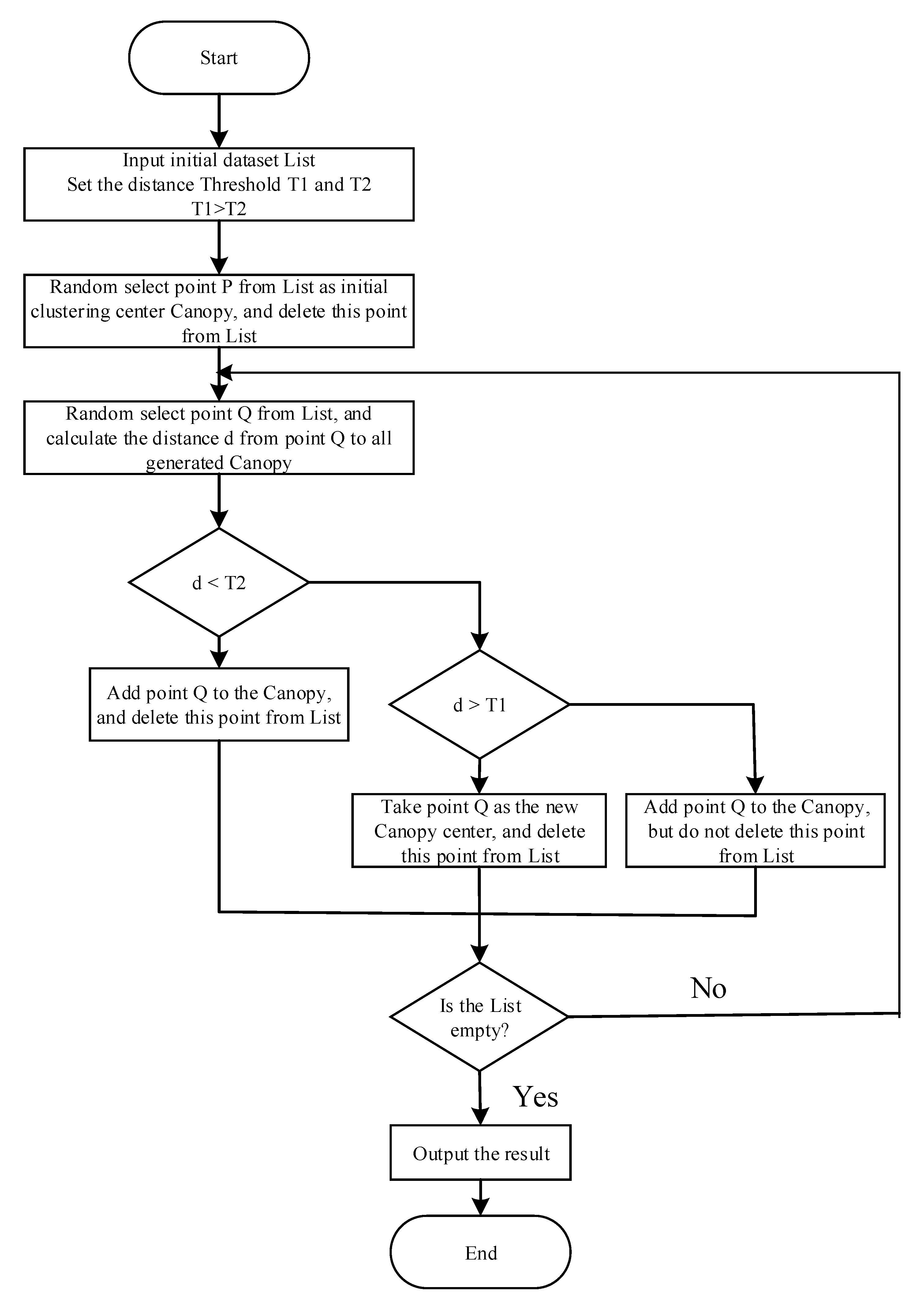
The specific steps of the Canopy algorithm are as follows:

(1)

Input the set List composed of original data and set the distance thresholds T1 and T2, where T1 > T2;

(2)

Randomly select data P from the List, use point P as the first data center Canopy and delete it from the List;

(3)

Take point Q from the set List, calculate the distance from Q to all Canopy that has been generated. If the distance to a Canopy is lower than T2, add Q to the Canopy and delete it from the List (think that the distance from Q point to this Canopy is close enough to not be the center of other Canopy); if the distance from Q to the center of all Canopy is greater than T1, then consider Q as a new Canopy and delete it from the List; If the distance from Q to the center of a Canopy is greater than T2 but lower than T1, add it to the Canopy, but not delete it from the List and continue to participate in the next calculation;

(4)

Repeat step 3 for other points in the set List until the set List is empty.

The flowchart of Canopy algorithm is as Figure 2.

Finally, the number of coarse cluster centers obtained by the Canopy algorithm is used as the input parameter of k-means algorithm to obtain the typical clustering result.

3. Typical Operating Scenario Generation Method

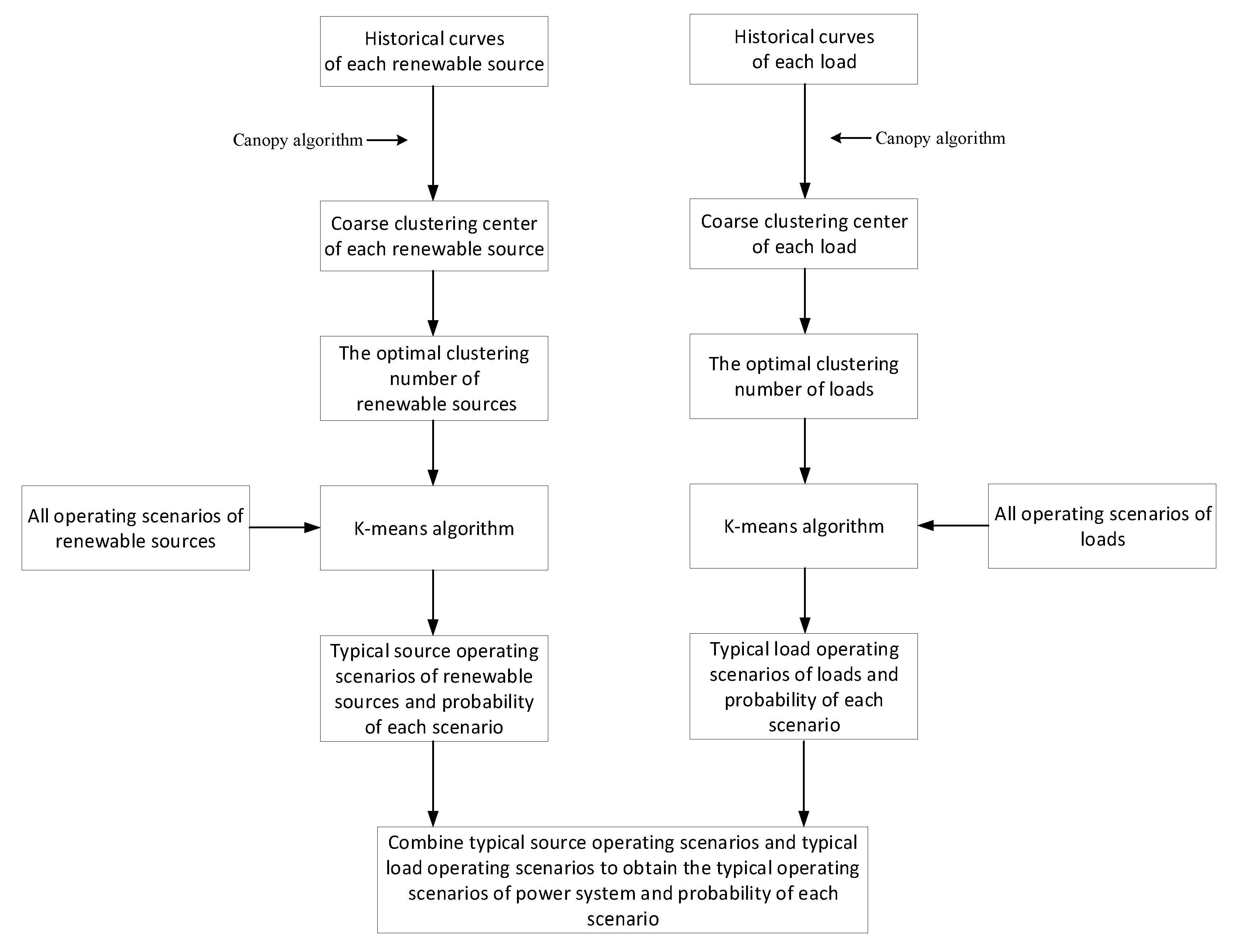
The growth of renewable energy in power systems and fluctuation of loads have brought great uncertainty to power systems. In a single year, there is no regularity to output scenarios of renewable energy. Therefore, it is necessary to cluster historical output scenarios in a given year to obtain typical output scenarios. However, if the proposed improved clustering method is performed on the historical output scenarios of each renewable energy source separately, the number of clustering scenarios for each power source may be different, increasing the complexity of calculations in subsequent analyses. Therefore, this study defines a power output operation scenario as follows: the output scenarios are obtained by taking all the renewable energy sources in the system as a whole; each power output operation scenario contains the output characteristic curve of each renewable energy source. The clustering process is completed by Canopy coarse clustering for each power source to obtain the optimal number of cluster centers. Then k-means clustering is performed on the power output operating scenarios to obtain the typical operating scenarios of renewable energy power sources. The specific process is as follows:

(1)

First, the historical curves of n renewable energy sources are respectively analyzed by Canopy coarse clustering to obtain the number of coarse cluster centers k_i (1 ≤ i ≤ n) of each power source. Then the number that appears most in k_i is found. This number is used as the optimal number k of clustering centers in a typical power operation scenario.

(2)

Then, using the optimal clustering number k as the input parameter of the next k-means, we use the clustering method to perform unified scenario clustering on the power output operating scenarios and obtain the typical operating scenarios of the power supply. At the same time, the occurrence probability P of each typical scenario can be obtained, according to the number of historical scenarios contained in each typical scenario. For example, given a daily curve of 365 days, with 365 historical scenarios, we cluster them to get 3 typical scenarios. If scenario 1 contains 100 historical scenarios, then 100/365 is the occurrence probability of scenario 1; scenario 2 and scenario 3 are the same.

The clustering process for a typical load scenario is similar to the clustering process for a power supply and is not repeated here.

After obtaining the clustering results of the power supply (assuming m typical scenarios) and the clustering results of load (assuming n typical scenarios), the typical scenarios of the power supply and the typical scenarios of the load are combined to obtain $m\times n$ typical system operating scenarios, as well as occurrence probabilities of each typical system operating scenario $P_i\times P_j$, where 1 ≤ i ≤ m, 1 ≤ j ≤ n.

In the typical system scenarios obtained, each output operating scenario of power supply is combined with all the load operating scenarios. Similarly, each operating scenario of load is also combined with all the power output operating scenarios, which basically covers possible scenarios of power system.

The process of generating typical system operating scenarios is shown in Figure 3.

4. Evaluation Index of Power System Flexibility

This study divides a power system into several zones, and divides flexibility evaluation into two levels: intra-zone and inter-zone. Intra-zone flexibility evaluation indices include upward/downward flexibility index of supply and demand in the zone and the grid flexibility index in the zone. Inter-zone flexibility evaluation indices include transmission channel flexibility indices of transmission channels between different zones.

4.1. Upward/Downward Flexibility Index of Supply and Demand in the Zone

The flexibility index of supply and demand is an index to determine whether flexibility of supply in the zone can meet the flexibility of demand in the zone.

The flexibility resources diagram of the zone is shown in Figure 4. In the zone, flexibility resources are divided into two parts: flexibility demand and flexibility supply. Flexibility demand is generated from uncontrollable parts, such as wind power, hydro power, photovoltaic power, exchange power and load power. Flexibility supply is generated from controllable parts such as thermal power and energy storage power.

4.1.1. Upward/Downward Flexibility Demand

For the moment t, the flexibility demand and supply of uncontrollable units of the zone are:

$$P_{uncon\_demand}\left(t\right)=P_{load}\left(t\right)+\Delta P\left(t\right)$$

(1)

$$P_{uncon\_\mathrm{supply}}\left(t\right)=P_{wind}\left(t\right)+P_{PV}\left(t\right)+P_{hydro}\left(t\right)$$

(2)

where, $P_{uncon\_demand}\left(t\right)$ is the flexibility demand of uncontrollable units; $P_{uncon\_\mathrm{supply}}\left(t\right)$ is the flexibility supply of uncontrollable units; $P_{load}\left(t\right)$, $P_{wind}\left(t\right)$, $P_{PV}\left(t\right)$, $P_{hydro}\left(t\right)$ are the load power, wind power, photovoltaic power and hydro power in the zone; $\Delta P\left(t\right)$ is the exchange power with other zones; when $\Delta P\left(t\right)>0$, this zone transmits power to other zones, increasing power demand; when $\Delta P\left(t\right)<0$, this zone receives power from other zones, reducing power demand.

The upper and lower limits of the power demand range at the moment t are shown in the following formula:

$$P_{uncon\_demand\_\max }\left(t\right)=\left(1+\lambda \right)P_{uncon\_demand}\left(t\right)-\left(1-\lambda \right)P_{uncon\_\mathrm{supply}}\left(t\right)$$

(3)

$$P_{uncon\_demand\_\min }\left(t\right)=\left(1-\lambda \right)P_{uncon\_demand}\left(t\right)-\left(1+\lambda \right)P_{uncon\_\mathrm{supply}}\left(t\right)$$

(4)

where, $P_{uncon\_demand\_\max }\left(t\right)$, $P_{uncon\_demand\_\min }\left(t\right)$ are the upper and lower limits of the power demand; $\lambda$ is the power fluctuation coefficient; The larger $\lambda$, the greater the power fluctuation.

Based on the above range of power demand, the calculation process of the flexibility demand of the zone is as follows.

When $P_{uncon\_demand\_\min }\left(t\right)>P_{uncon\_demand}\left(t-1\right)$, there is only upward flexibility demand:

$$P_{demand\_up}\left(t\right)=P_{uncon\_demand\_\max }\left(t\right)-P_{uncon\_demand}\left(t-1\right)$$

(5)

When $P_{uncon\_demand\_\max }\left(t\right)>P_{uncon\_demand}\left(t-1\right)>P_{uncon\_demand\_\min }\left(t\right)$, there are both upward and downward flexibility demand:

$$P_{demand\_up}\left(t\right)=P_{uncon\_demand\_\max }\left(t\right)-P_{uncon\_demand}\left(t-1\right)$$

(6)

$$P_{demand\_down}\left(t\right)=P_{uncon\_demand}\left(t-1\right)-P_{uncon\_demand\_\min }\left(t\right)$$

(7)

When $P_{uncon\_demand}\left(t-1\right)>P_{uncon\_demand\_\max }\left(t\right)$, there is only downward flexibility demand:

$$P_{demand\_down}\left(t\right)=P_{uncon\_demand}\left(t-1\right)-P_{uncon\_demand\_\min }\left(t\right)$$

(8)

where, $P_{demand\_up}\left(t\right)$, $P_{demand\_down}\left(t\right)$ are upward flexibility demand and downward flexibility demand of the zone; $P_{uncon\_demand}\left(t-1\right)$ is the flexibility demand of uncontrollable parts at previous moment.

4.1.2. Upward/Downward Flexible Supply

The zone′s upward/downward flexibility supply is provided by controllable parts. The calculation of the zone′s upward/downward flexibility supply is as follows.

$$P_{\mathrm{supply}\_\mathrm{up}}\left(t\right)=P_{\mathrm{con}\_\mathrm{gen}\_\max }-P_{con\_gen}\left(t\right)$$

(9)

$$P_{\mathrm{supply}\_\mathrm{down}}\left(t\right)=P_{con\_gen}\left(t\right)-P_{\mathrm{con}\_\mathrm{gen}\_\min }$$

(10)

where, $P_{\mathrm{supply}\_\mathrm{up}}\left(t\right)$, $P_{\mathrm{supply}\_\mathrm{down}}\left(t\right)$ are upward flexibility supply and downward flexibility supply of the zone; $P_{\mathrm{con}\_\mathrm{gen}\_\max }$ is the maximum output of all controllable units; $P_{\mathrm{con}\_\mathrm{gen}\_\min }$ is the minimum output of all controllable units; $P_{con\_gen}\left(t\right)$ is the output value of controllable units at the moment.

According to the upward/downward flexibility demand and supply mentioned above, we can obtain the supply and demand flexibility index.

The upward flexibility index of supply and demand is:

$$F_{up}\left(t\right)=\frac{P_{demand\_up}\left(t\right)}{P_{\mathrm{supply}\_up}\left(t\right)}$$

(11)

The upward flexibility index of supply and demand represents the ability of the upward flexibility supply to meet the upward flexibility demand. When the index is lower than 1, the upward flexibility supply is greater than the upward flexibility demand, and there is still a certain margin for the flexibility supply. When the index is greater than 1, the upward flexibility supply is less than the upward flexibility demand. The flexibility supply may not be able to meet the demand of the power system. Certain measures need to be taken in the future planning stage (configuration of controllable units, energy storage, renewable energy or load shedding, etc.) to ensure a balance between flexibility supply and demand.

The downward flexibility index of supply and demand is:

$$F_{down}\left(t\right)=\frac{P_{demand\_down}\left(t\right)}{P_{\mathrm{supply}\_down}\left(t\right)}$$

(12)

The downward flexibility index of supply and demand represents the ability of the downward flexibility supply to meet the downward flexibility demand. When the index is lower than 1, the downward flexibility supply is greater than the downward flexibility demand and there is still a certain margin for the flexibility supply. When the index is greater than 1, the downward flexibility supply is less than the downward flexibility demand. The flexibility supply may not be able to meet the demand of the power system. Certain measures need to be taken in the future planning stage (reduce renewable energy, increase load, etc.) to ensure a balance between flexibility supply and demand.

4.2. Grid Flexibility Index of the Grid in the Zone

The growth of renewable energy affects the power flow distribution of the system. The grid flexibility index is an index to determine whether the grid structure and line transmission capacity in the zone can meet the power flow distribution.

The grid flexibility index is based on N branches with the highest load rate in the grid at time t and the weighted average of the load rate is used as the grid flexibility index at time t.

$$\mathrm{Flex}\_\mathrm{net}(t)={\displaystyle \sum _{i=1}^N{\mu }_i{L}_i}\left(t\right)$$

(13)

where, $\mathrm{Flex}\_\mathrm{net}(t)$ is the grid flexibility at moment t; N is the number of branches selected; ${\mu }_i$ is the flexibility weight factor for branch i; $L_i\left(t\right)$ is the load rate of branch i at moment t.

The load rate is:

$$L_i\left(t\right)=\frac{S_i\left(t\right)}{S_{i\max }}$$

(14)

where, $S_i\left(t\right)$ is the transmission capacity of branch i; $S_{i\max }$ is the maximum transmission capacity of branch i.

If the load rate of the branch is greater than 1, an overload situation will occur in actual operation. Corresponding measures (abandon wind, light and load shedding) will need to be taken. If the load rate of the branch is lower than 1, the branch can operate normally.

The definition of the flexibility weight factor ${\mu }_i$ is:

$${\mu }_i=\frac{{\sigma }_{\mathrm{i}}^2}{{\displaystyle \sum _{i=1}^N{{\sigma }_i}^2}}=\frac{{{\displaystyle \sum _{t=1}^T\left(L_i\left(t\right)-\overline{L_i}\right)}}^2}{{\displaystyle \sum _{i=1}^N{\displaystyle \sum _{t=1}^T{\left(L_i\left(t\right)-\overline{L_i}\right)}^2}}}$$

(15)

where, ${\sigma }_i^2$ is the variance of the load rate of branch i; $\overline{L_i}$ is the average load rate of branch i at all moments; N and T are the maximum number of branches and the maximum number of moments.

The significance of ${\mu }_i$ lies in the horizontal comparison of the ability of each branch to withstand the impact of flexibility resource fluctuations and identify the ‘weak point’ that really restricts the flexibility of the grid.

According to the definition, $\mathrm{Flex}\_\mathrm{net}(t)$ is greater than 0. When $\mathrm{Flex}\_\mathrm{net}(t)>1$, in actual operation, one or more branches will be overloaded, and corresponding measures need to be taken to respond. The lower the $\mathrm{Flex}\_\mathrm{net}(t)$, the better the grid flexibility.

4.3. Transmission Channel Flexibility Index Between the Zones

For some zones, there are too many renewable energy sources, and too little load. The demand in the zone cannot consume the electricity generated by renewable energy sources, and a large amount of electricity needs to be transmitted to external zones. Therefore, the flexibility index of the transmission channel is defined to determine whether the transmission capacity of the transmission channel can meet the transmitted power.

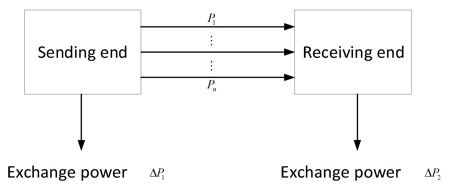
According to the power flow relationship between zones, the two ends of the transmission channel are divided into the sending end and the receiving end; the power flow direction is shown in Figure 5. Assume that there are n transmission lines between the sending end and the receiving end. The active power of each transmission line is defined as $P_1,\dots ,P_n$, and they constitute a transmission channel.

For the sending end, at moment t, its sending power is:

$$P_{send}\left(t\right)=P_{wind}\left(t\right)+P_{PV}\left(t\right)+P_{hydro}\left(t\right)+P_{con\_gen}\left(t\right)-P_{load}\left(t\right)-\Delta P\left(t\right)$$

(16)

where, $P_{send}\left(t\right)$ is the sending power of the sending end.

4.3.1. Normal Operating Condition

Ignoring the transmission loss, the transmission power of the sending end is the transmission power of the inter-regional transmission channel:

$$P_{send}\left(t\right)=P_{trans}\left(t\right)=P_1\left(t\right)+P_2\left(t\right)+\dots +P_n\left(t\right)$$

(17)

where, $P_{trans}\left(t\right)$ is the transmission power of the transmission channel; $P_1\left(t\right),\dots ,P_n\left(t\right)$ are the transmission power of line 1 to line n.

Define the power distribution coefficient of each transmission line in the transmission channel as r, then the total transmission power of the transmission channel is:

$$\begin{array}{ll}{P}_{trans}\left(t\right)& =P_1\left(t\right)+P_2\left(t\right)+\dots +P_n\left(t\right)\\ & =r_1{P}_{trans}\left(t\right)+r_2{P}_{trans}\left(t\right)+\dots +r_n{P}_{trans}\left(t\right)\\ & ={\displaystyle \sum _{i=1}^n{r}_i{P}_{trans}\left(t\right)}\end{array}$$

(18)

where, $r_i$ is the power distribution coefficient of transmission line i and ${\displaystyle \sum _{i=1}^n{r}_i}=1$.

Under different operating scenarios of the system, the power distribution coefficients of the transmission lines are different, but under the same operating scenario, the power distribution coefficients of the transmission lines are considered to be the same.

The definition of power distribution coefficient is:

$$r_i=\frac{\overline{P_i}}{{\displaystyle \sum _{i=1}^n\overline{P_i}}}$$

(19)

$$\overline{P_i}=\frac{1}{T}{\displaystyle \sum _{t=1}^T{P}_i\left(t\right)}$$

(20)

where, $P_i\left(t\right)$ is the power of transmission line i at moment t; $\overline{P_i}$ is the average power of transmission line i at all moments.

If one of all transmission lines in the transmission channel reaches the upper limit of the transmission power, which is:

$$r_i{P}_{trans}\left(t\right)=P_{\mathrm{i}\max }$$

(21)

where, $P_{i\max }$ is the upper limit of the transmission power of line i.

At this time, it is considered that the total transmission power between the sending end and the receiving end has reached the maximum value. We calculate the value of the transmission channel when each line reaches the upper power limit and take the minimum value as the upper limit of the transmission channel capacity.

$$P_{normal\_\max }=\min \left\{\frac{P_{1\max }}{r_1},\dots ,\frac{P_{i\max }}{r_i}\right\}$$

(22)

where $P_{normal\_\max }$ is the maximum transmission power of the transmission channel.

Define the maximum output power at the sending end as

$$\begin{array}{ll}{P}_{source\_\max }& =\max \left\{t|P_{wind}\left(t\right)+P_{\mathrm{PV}}\left(t\right)+P_{\mathrm{hydro}}\left(t\right)\right\}+\min \left\{t|P_{con\_gen}\left(t\right)\right\}\\ & -\min \left\{t|P_{load}\left(t\right)\right\}-\min \left\{\Delta P\left(t\right)\right\}\end{array}$$

(23)

where $P_{source\_\max }$ is the maximum output power of the sending end.

At normal operating condition, the transmission channel flexibility index is:

$$F_{channel}=\frac{P_{source\_\max }}{P_{normal\_\max }}$$

(24)

A value of $F_{channel}>1$ indicates that the flexibility of the transmission channel is insufficient under normal operating condition and it cannot meet the transmission demand of the maximum output power of the sending end, a new transmission line needs to be added.

A value of $F_{channel}=1$ indicates that the transmission channel just meets the transmission demand of the maximum output power at the sending end under normal operating condition.

A value of $F_{channel}<1$ indicates that the flexibility of the transmission channel is sufficient under normal operating condition and the power output at the sending end is not blocked.

4.3.2. N-1 Operating Condition

If the line k in the transmission channel fails, at this time only n − 1 transmission lines are operating between the sending end and the receiving end; the total transmission power of the transmission line is:

$$\begin{array}{ll}{P}_{trans}\left(t\right)& =P_1\left(t\right)+P_2\left(t\right)+\dots +P_n\left(t\right)\\ & =r_1{P}_{trans}\left(t\right)+r_2{P}_{trans}\left(t\right)+\dots +r_n{P}_{trans}\left(t\right)-r_k{P}_{trans}\left(t\right)\\ & ={\displaystyle \sum _{i=1,i\ne k}^n{r}_i{P}_{trans}\left(t\right)}\end{array}$$

(25)

The power distribution coefficient is:

$$r_i=\frac{\overline{P_i}}{{\displaystyle \sum _{i=1}^n\overline{P_i}}}\left(i\ne k\right)$$

(26)

$$\overline{P_i}=\frac{1}{T}{\displaystyle \sum _{t=1}^T{P}_i\left(t\right)}\left(i\ne k\right)$$

(27)

If one of the n − 1 transmission lines in the operating state reaches the upper power limit, it is considered that the total transmission power between the sending end and the receiving end has reached the maximum value. We calculate the value of the transmission channel when each line reaches the upper power limit and take the minimum value as the upper limit of the transmission channel capacity.

$$P_{k\_fault\_\max }=\underset{i\ne k}{\min }\left\{\frac{P_{1\max }}{r_1},\dots ,\frac{P_{i\max }}{r_i}\right\}$$

(28)

where, $P_{k\_fault\_\max }$ is the maximum transmission power of transmission channel when the line k fails.

In each operating situation, calculate the maximum transmission power of the remaining lines when each line in the transmission channel fails and take the minimum value of the maximum transmission power as the upper limit of the transmission power of the transmission channel under N-1 operating conditions between the two zones.

$$P_{fault\_\max }=\underset{1<k<n}{\min }\left\{P_{k\_fault\_\max }\right\}$$

(29)

where, $P_{fault\_\max }$ is the maximum transmission power of the transmission channel under N-1 operating condition.

Under N-1 conditions, the transmission channel flexibility index is:

$$F_{channel\_fault}=\frac{P_{source\_\max }}{P_{fault\_\max }}$$

(30)

A value of $F_{channel}>1$ indicates that the flexibility of the transmission channel is insufficient under N-1 operating condition and it cannot meet the transmission demand of the maximum output power of the sending end and a new transmission line needs to be added.

A value of $F_{channel}=1$ indicates that the transmission channel just meets the transmission demand of the maximum output power at the sending end under N-1 operating condition.

A value of $F_{channel}<1$ indicates that the flexibility of the transmission channel is sufficient under N-1 operating condition and the power output at the sending end is not blocked.

4.4. Flexibility Assessment Process

Based on the improved k-means algorithm, this study generates several typical scenarios, analyzes the flexibility evaluation results of each typical scenario and weights the comprehensive flexibility evaluation indices according to the probability of each typical scenario. The specific flowchart is shown in Figure 6.

5. Case Study

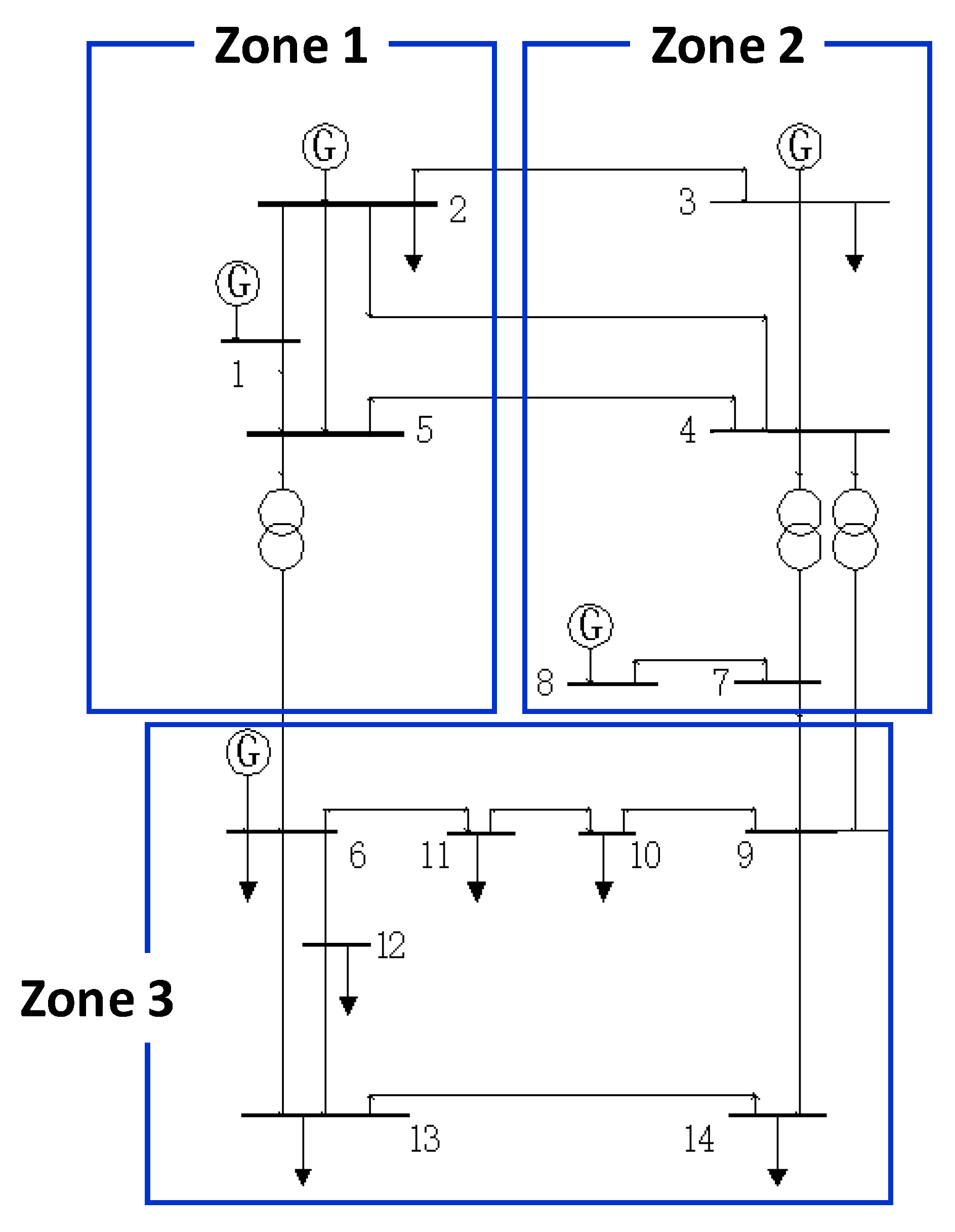
In this section—based on the historical output data of a Power Grid—a modified IEEE 14-node test system was used to evaluate the flexibility. The case was divided the test system into three zones, as shown in Figure 7. The configuration of renewable power sources is shown in

Table 1. System Renewable Power Configuration.

Unit Type	Node	Capacity (MW)
Wind power	1	100
Wind power	2	120
Wind power	3	50
Photovoltaic power	6	50
Hydro power	8	50

. Controllable units were connected to nodes 2, 3, 6; total installed capacity was 1000 MW. The total installed capacity of renewable power sources was 370 MW. Volatile loads were connected to nodes 2, 3, 6, 8, 10, 12, 13 and 14. In each scenario—except for nodes connected to renewable energy and volatile loads—the power and load of other nodes were fixed. The maximum capacity of the transmission lines between Zone 1 and Zone 2 was 200 MVA, the maximum capacity of the transmission lines of Zone 1 and Zone 3 was 200 MVA and the maximum transmission line capacity of the Zone 2 and Zone 3 was 100 MVA. Power fluctuation coefficient $\lambda$ was taken as 0.2.

5.1. Typical Scenario Generation Results

In this section, the historical curve of renewable power sources and loads throughout the year was used as the basic data for clustering to obtain daily curves of typical scenarios. Each curve contained 24 moments.

First, we determined the optimal number of cluster centers for renewable power sources and loads. The Canopy algorithm was used to perform coarse clustering on the annual historical curve of each renewable power source and load, to obtain the number of coarse cluster centers, as shown in

Table 2. Coarse Clustering Number of Renewable Sources.

	Node 1	Node 2	Node 3	Node 6	Node 8
Coarse clustering number of each source	3	3	4	3	4
The optimal clustering number of sources	3

and

Table 3. Coarse Clustering Number of Loads.

	Node 2	Node 3	Node 6	Node 8
Coarse clustering number of each load	3	5	3	4
	Node 10	Node 12	Node 13	Node 14
Coarse clustering number of each load	5	3	3	3
The optimal clustering number of loads	3

.

According to the result of coarse clustering, the optimal clustering number of renewable power source operating scenarios and the optimal clustering number of load operating scenarios were both 3. The output curve of each source is shown as Figure 8.

The k-means clustering was performed to obtain three typical power source output scenarios and the probability of each scenario. According to the output of the power source, the three scenarios were divided into three types: source peak, source level and source valley. Then, the load operating scenarios were clustered by k-means algorithm, which also yielded three typical load types: load peak, load level and load valley. We combined typical source output scenarios and typical load scenarios to get 9 typical system scenarios. The probability of each system scenario is shown in

Table 4. Probability of Typical Scenarios of System.

Source Scenario	Probability	Load Scenario	Probability	System Scenario	Probability
Scenario 1 (Source peak)	0.45	Scenario 1 (Load peak)	0.29	Scenario 1 (Source peak and load peak)	0.1305
				Scenario 2 (Source peak and load level)	0.189
				Scenario 3 (Source peak and load valley)	0.1305
Scenario 2 (Source level)	0.32	Scenario 2 (Load level)	0.42	Scenario 4 (Source level and load peak)	0.0928
				Scenario 5 (Source level and load level)	0.1344
				Scenario 6 (Source level and load valley)	0.0928
Scenario 3 (Source valley)	0.23	Scenario 3 (Load valley)	0.29	Scenario 7 (Source valley and load peak)	0.0667
				Scenario 8 (Source valley and load level)	0.0966
				Scenario 9 (Source valley and load valley)	0.0667

.

5.2. Analysis of Supply and Demand Flexibility Index Results in the Zone

We were able to obtain the power flow of a given scenario at each moment according to the power output values and load output values at each moment in the scenario. Then, according to the power flow results, power output values and load output values at each moment in each scenario, we used the calculation method of flexibility index of supply and demand in the zone to determine the flexibility index curve of each scenario. Finally, we calculated the comprehensive supply and demand flexibility indices based on the occurrence probability of each scenario. The upward/downward supply and demand flexibility indices are shown in Figure 9.

As is seen in Figure 9a, the upward flexibility indices of Zone 1 and Zone 2 were both rising first, and then decreasing. At some times during the day, the upward flexibility indices were greater than 1, indicating that the upward flexibility supply at these moments cannot meet upward flexibility demand. This was because the renewable energy of Zone 1 was mainly wind power. The output of wind power will decrease during the day. With the decrease of wind power output, renewable energy was unable to meet the load demand more and more. And the upward flexibility demand increased, which made the upward flexibility indices gradually worsen. The renewable energy sources in Zone 2 were mainly wind power and hydropower. Hydropower can make up for some wind power output. At the same time, the load demand in Zone 2 was smaller, so the upward flexibility indices of Zone 2 were slightly better than those in Zone 1. The upward flexibility indices in Zone 3 were decreasing first and then increasing. This was because the renewable energy of Zone 3 was photovoltaic and the output at night was basically 0. Therefore, the upward flexibility demand was met by the controllable units in Zone 3, so the upward flexibility indices at night were poor, and daytime indices were better.

From the Figure 9b, the downward flexibility indices of Zone 1 and Zone 2 were lower than 1, indicating that the downward flexibility supply can meet the downward flexibility demand at each moment, and there was no risk of abandoning renewable energy. However, the downward flexibility index of Zone 3 at moment 13 was greater than 1, which indicates that the downward flexibility supply of Zone 3 at this moment cannot meet the downward flexibility demand. This was because the output of PV power in Zone 3 increases rapidly, and the load demand in Zone 3 was insufficient. Therefore, the downward flexibility demand increases, and there was not enough capacity for controllable units to meet the downward flexibility, and there was a risk of abandoning renewable energy.

From Figure 9, the upward flexibility indices and the downward flexibility indices were opposite.

5.3. Analysis of Supply and Demand Flexibility Index Results of the Whole System

From Figure 10, the upward flexibility indices of this system were poor, while the downward flexibility indices were good. According to Figure 9a and Figure 10a, the upward flexibility indices of the whole system at some moments were lower than 1, but at these moments, the upward flexibility indices of some zones were actually very large. According to Figure 9b and Figure 10b, the downward flexibility indices of the whole system were lower than 1 at all moments, but the downward flexibility indices of some zones were high at some moments. This indicates that when the flexibility indices of the whole system meet the requirements, there was actually a situation where the flexibility supply cannot meet the flexibility demand at some zones. Therefore, when analyzing the supply and demand flexibility index, it was necessary to analyze the system based on different zone characteristics.

With the increasing proportion of renewable energy in the future, the uncertainty of its output may lead to situations such as load shedding or abandonment of renewable energy. Therefore, by analyzing the supply and demand flexibility indicators of each zone, planning and other means can be used to avoid situations that are not conducive to system operation. For zones with poor downward flexibility index, energy storage equipment can be configured to cut peaks, and the transmission channel can be constructed appropriately to transfer excess energy from this zone to external zones. For zones with poor upward flexibility index, when planning in the future, the flexibility needs can be matched by configuring controllable flexibility resources such as energy storage, thermal power and reservoirs.

5.4. Analysis of Grid Flexibility Index of the Zone

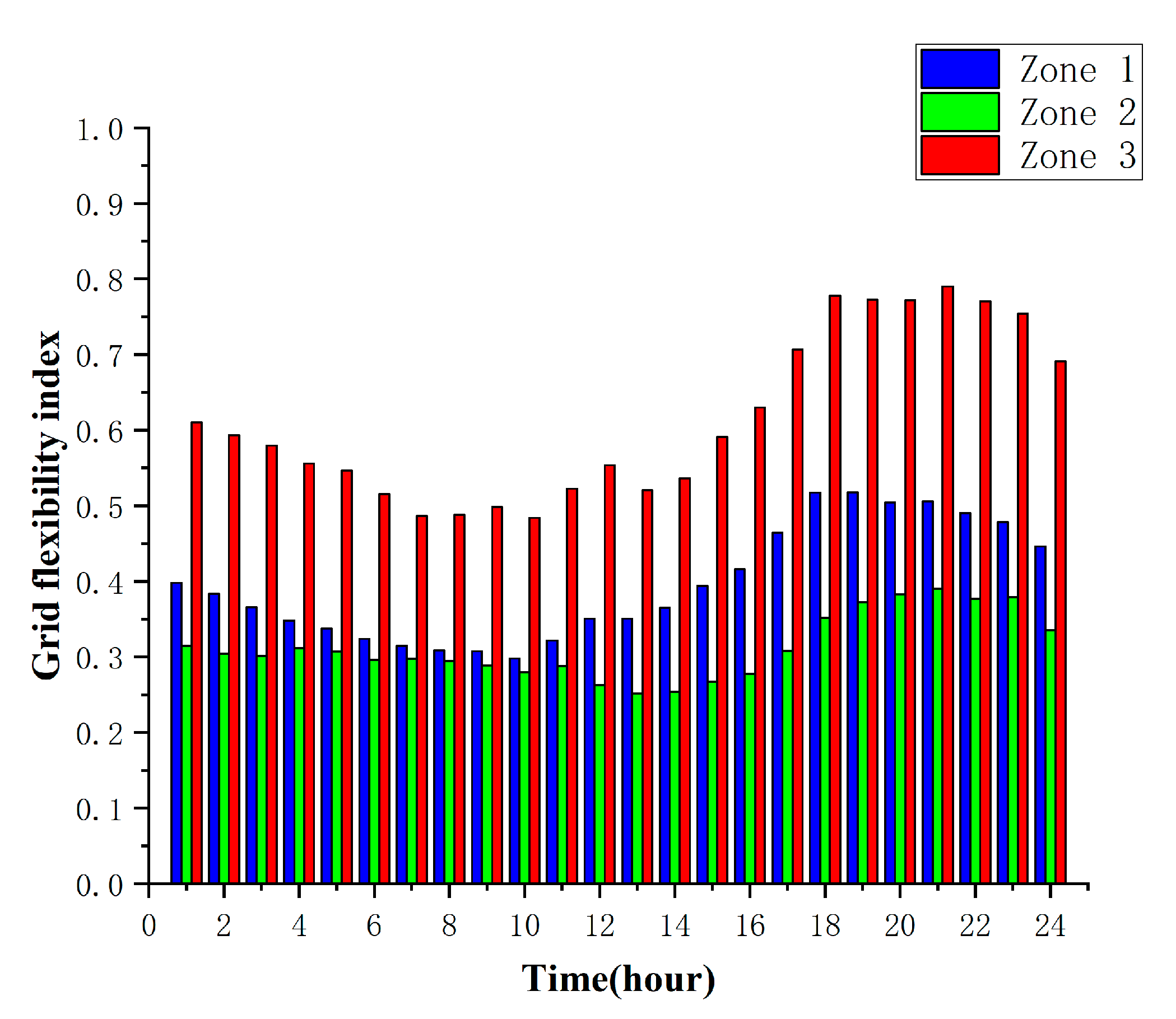
According to the calculation results of the whole system power flow, choose the first 30% of branches with the highest load rate in each zone to calculate the grid flexibility index of each zone.

From Figure 11, the grid flexibility indices of these Zones were all lower than 1, which indicates that they were in normal operating state, and there was almost no line overload. The maximum transmission capacity of the lines in the zone can meet the power flow distribution. The grid flexibility indices of Zone 3 were greater than indices of Zone 1 and Zone 2, which indicates that the lines with the highest load rate in Zone 3 were in high load rate at some moments. If the load demand and the renewable energy increase in the future, the grid flexibility index in Zone 3 will become worse, and the maximum capacity of the lines needs to be increased to meet the power flow distribution requirements.

5.5. Comprehensive Analysis of Supply and Demand Flexibility Index and Grid Flexibility Index

From Figure 9 and Figure 11, the grid flexibility indices of the three zones were lower than 1, indicating that the line capacity of the three zones can meet the power flow distribution, but the upward or downward flexibility indices of the three zones were too large at some moments. It shows that the grid flexibility index cannot fully reflect the flexibility of the zone. When the grid flexibility index meets the requirements, the capacity of the line can withstand the power flow, but the power and load output do not match. If the power output is increased in the future, it is possible that the power and load can be matched, but the transmission capacity of the line will not be able to withstand the corresponding power flow distribution, and the power supply will not be able to transmit to the demand. Therefore, it was necessary to analyze the supply and demand flexibility index and the grid flexibility index comprehensively to obtain the zone′s flexibility status, only when both indices meet the requirements, the zone’s flexibility is good.

With the increasing loads in the future, in order to meet the system’s supply and demand balance, the proportion of renewable energy will also increase correspondingly which will adversely affect the safe and stable operation of the system. Through the supply and demand flexibility index and the grid flexibility index, the system’s supply and demand balance and the margin of line transmission capacity can be judged, so as to comprehensively evaluate the flexibility status of the system.

5.6. Analysis of Transmission Channel Flexibility Index Between the Zones

Using the proposed calculation method of transmission channel flexibility index, the calculation results of transmission channel flexibility index between different zones in different typical scenarios of the system can be obtained, as shown in

Table 5. Transmission Channel Flexibility Index.

	Zone1–Zone2		Zone1–Zone3		Zone2–Zone3
	Normal	N-1	Normal	N-1	Normal	N-1
Scenario 1	0.3860	0.7363	0.8297	1.3525	0.8419	/
Scenario 2	0.4375	0.8239	0.8456	1.3914	0.8189	/
Scenario 3	0.4087	0.8139	0.8778	1.3593	0.8003	/
Scenario 4	0.3545	0.7550	0.8109	1.3357	0.8936	/
Scenario 5	0.3574	0.7264	0.7987	1.2837	0.8263	/
Scenario 6	0.3678	0.7342	0.7936	1.2854	0.8298	/
Scenario 7	0.4345	0.6970	0.7293	1.1276	0.8920	/
Scenario 8	0.3955	0.7044	0.7139	1.3937	0.8404	/
Scenario 9	0.3866	0.7232	0.7778	1.3574	0.9123	/

.

According to the results in Table 5, in all scenarios, the transmission channel flexibility indices under normal operating conditions from Zone 1 to Zone 2, Zone 1 to Zone 3 and Zone 2 to Zone 3 were all lower than 1, indicating that the maximum transmission capacity of the transmission channels between these zones can meet the maximum output of the sending end, and the output of the sending end was not blocked.

Under N-1 operating conditions, the transmission channel flexibility indices from Zone 1 to Zone 2 were still lower than 1, indicating that when a certain line fails, the maximum transmission capacity of the transmission channel can still meet the maximum output of the sending end. But the transmission channel flexibility indices from Zone 1 to Zone 3 under N-1 conditions were greater than 1, indicating that when a line in the transmission channel fails, the transmission channel cannot meet the maximum sending power. More lines need to be constructed to improve transmission capacity of transmission channel. And there was only one line for the transmission channel from Zone 2 to Zone 3. If this line fails suddenly, the output power of Zone 2 cannot be transmitted to Zone 3. Under normal conditions, the transmission channel indices from Zone 2 to Zone 3 were close to 1, indicating that the transmission capacity was not sufficient and has a high risk of transmission congestion. The best way to deal with this problem was to construct more lines between Zone 2 and Zone 3 to improve the transmission capacity.

If the power output cannot be transmitted, it will increase the renewable energy abandonment rate; if it is forced to consume internally, it may also affect the power flow distribution, increase the load rate of the lines in the zone, increase the risk of overload of the lines in the zone and affect the safety and stability of the system. Therefore, as the output of renewable energy gradually increases, the maximum power output of the sending zone will increase. It is necessary to expand the maximum transmission capacity of the transmission channel or expand the lines to meet the external transmission demand of electricity, and at the same time, the renewable energy abandonment rate in the sending zone can also be reduced.

5.7. Rationality of the Clustering Method

This section studies the effectiveness of the clustering method. First, based on the flexibility evaluation results of each scenario and the weighted calculation of each scenario’s occurrence probability, the comprehensive flexibility indices were obtained. Then, based on the power and load history data of the whole year, the flexibility indices were obtained for the whole year. Finally, the evaluation results of two methods were compared to verify the rationality of the clustering results.

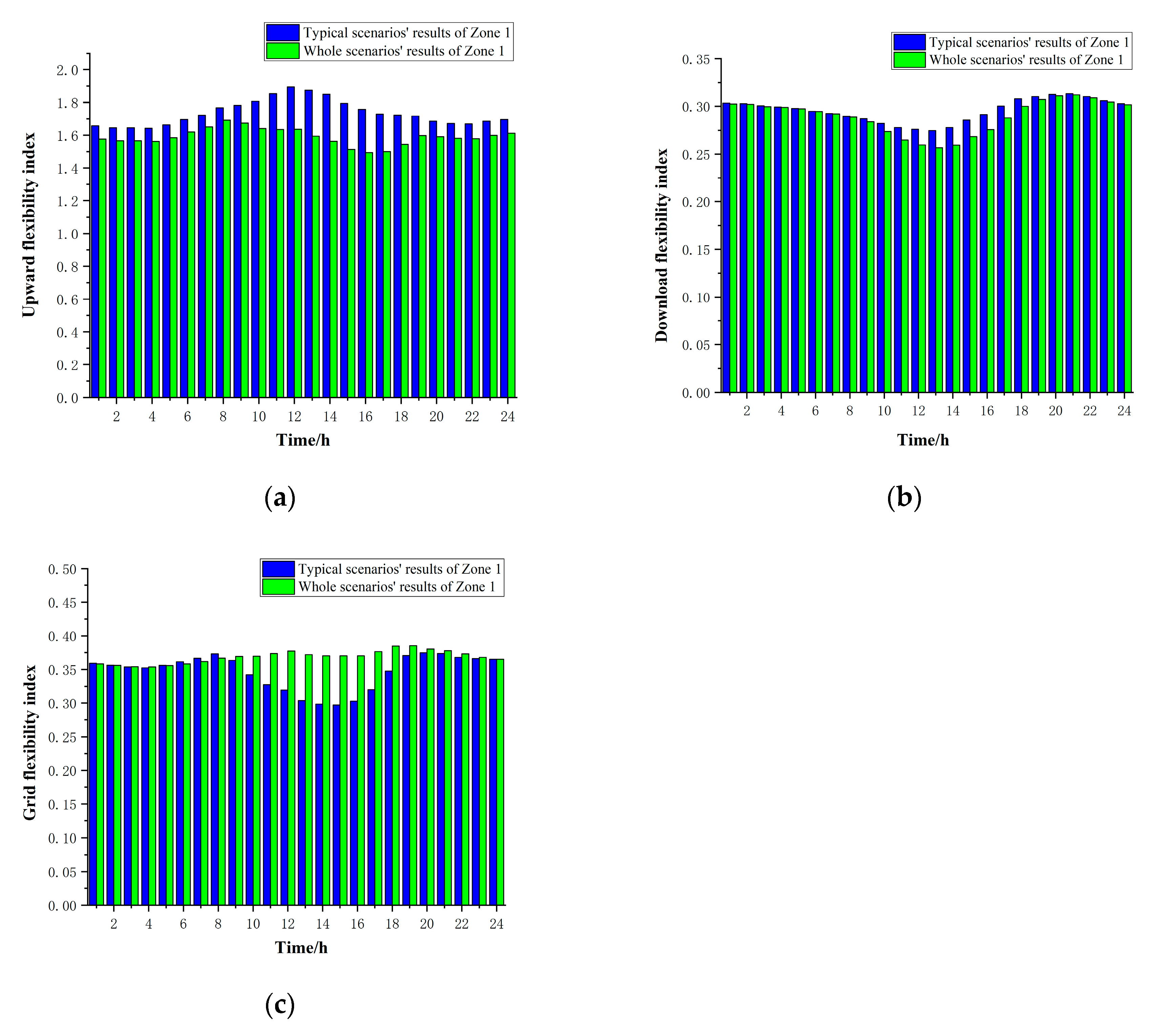
Take Zone 1 as an example—it can be seen from Figure 12 that the flexibility indices of two methods were relatively close. Although not all indices were close at each moment, the overall trend was consistent. The comprehensive flexibility evaluation indices obtained based on the clustering scenario can accurately reflect the system′s flexibility in a certain period of time. Therefore, the typical scenario generation method proposed in this paper can greatly reduce the calculation time and improve the efficiency of flexibility evaluation without affecting the accuracy of the evaluation results.

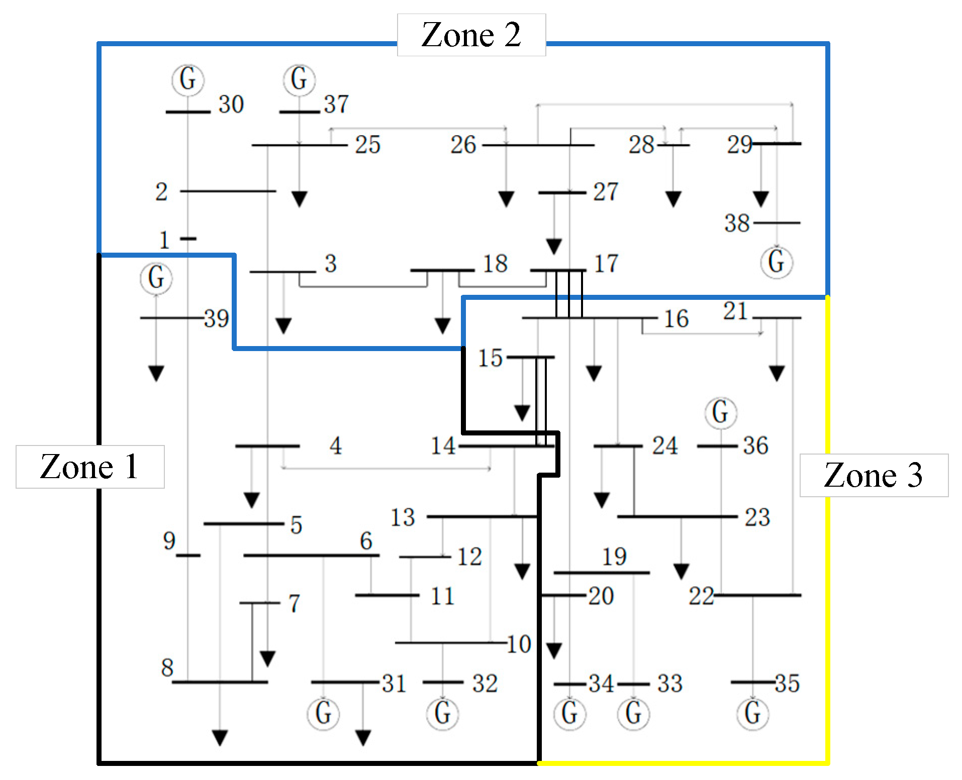
5.8. Evaluation on Modified IEEE 39-Node System

In order to verify the effectiveness of the methodology proposed in this paper, a modified IEEE 39-node system was also used to evaluate the flexibility. The zone figure is as Figure 13. The renewable power sources configuration is as

Table 6. System Renewable Power Configuration.

Unit Type	Node	Capacity(MW)
Wind power	32	200
Wind power	33	300
Wind power	34	100
Photovoltaic power	35	100
Hydro power	37	100

. The trends of the power sources and loads were consistent with 14-nodes case above, but the installed capacity of power sources has been expanded.

Using Zone 1 as an example, the results are as Figure 14. It can be seen from Figure 14a,b that the upward supply and demand flexibility indices of Zone 1 were larger than 1 and relatively, the downward supply and demand flexibility indices of Zone 1 were lower than 1, indicating that in the future, more flexible resources such as thermal power and energy storage systems need to be configured in Zone 1 to increase the upward adjustment ability. And from Figure 14c, it can be seen that the grid flexibility indices of Zone 1 were lower than 1, which means that the transmission lines in Zone 1 were in normal operating state, and there was almost no line overload. The maximum transmission capacity of the lines in the zone can meet the power flow distribution. From these three figures, the results obtaining by the typical scenarios proposed in this paper and the results obtaining by the whole scenarios were relatively close, and the overall trend was consistent. Therefore, the results of the IEEE 14-node case and IEEE 39-node case support that the method proposed in this paper can effectively reflects the flexibility status of the power system and improve the efficiency of flexibility evaluation.

6. Conclusions

This paper proposes the method of power system flexibility evaluation. First, a clustering method of renewable energy and load operating scenarios was studied. The results of the cases showed that the improved k-means clustering method can reduce a large amount of historical data into several typical operating scenarios.

At the same time—from the perspective of supply and demand balance, power flow distribution and transmission capacity, flexibility evaluation indices of the power system were proposed, and flexibility evaluation was performed, based on typical operating scenarios. The calculation results show that the proposed indices reflect the flexibility status of the power system. Typical operating scenarios can represent the flexibility of all the operating scenarios of the power system throughout the cycle, thereby improving the flexibility evaluation efficiency.

The flexibility evaluation method proposed in this article can provide advice for the planning and configuration of power systems. Future work will further consider the power system optimization configuration research based on the results of the flexibility evaluation, and consider the influence of energy storage systems to improve the future power system operation flexibility, and ensure that the power system can operate safely with a high proportion of renewable energy access.