Abstract
Recently, demand-side resources (DSRs) have proceeded to participate in frequency control of the power systems. Compared with traditional generation-side resources, DSRs have unique intermittent characteristics. Taking aggregation of air conditions as an example, they must take a break after providing power support for a period of time considering the user comfort. This behavior, known as the intermittent characteristic, obviously affects the stability of the power systems. Therefore, this paper designs a corresponding controller for DSRs based on the intermittent control method. The designed controller is incorporated into the traditional load frequency control (LFC) system. The time delay is also considered. A rigorous stability proof and the robust performance analysis is presented for the new LFC system. Then, the sufficient robust frequency stabilization result is presented in terms of linear matrix inequalities (LMIs). Finally, a two-area power system is provided to illustrate the obtained results. The results show that the designed intermittent controller can mitigate the impact of intermittent characteristics of DSRs.
1. Introduction
As one of the essential indicators of power systems, frequency is often used to evaluate the safety and stability of power systems. To keep the frequency near the rated value, many scholars not only designed the control strategy for the generation-side resources [1], but also pointed out that demand-side resources can participate in frequency control [2,3]. These studies have shown that when the power systems suffer from a large disturbance, DSRs can support the stability more quickly and flexibly than generation-side resources. Therefore, DSRs have great potential for future frequency control in the power systems [4].
In the past few years, researchers have proposed a variety of control modes for DSRs [5]. From the perspective of the DSRs providers, there are three control modes for DSRs to participate in the frequency control: centralized [6], decentralized [7,8,9] and distributed [10]. From the perspective of the grid dispatch center, DSRs need be used for different frequency control scenarios: emergency control [11], primary control [7,12,13] and secondary control [14,15]. Under different frequency control scenarios, in order to achieve the best control performance, the control mode of DSRs should be selected differently.
As the study progresses, researchers are gradually finding that it is not enough to consider only the control mode of DSRs. The characteristics of DSRs are diversified and will significantly affect the frequency control performance. Therefore, some researchers have designed corresponding control strategies for different characteristics. Considering the communication delay characteristics of DSRs, S. Ali Pourmousavi et al. [16,17] first propose the single-area and multi-area models of DSRs participating in the load frequency control (LFC) system. Then, Yi et al. [18] treated time delay as an inertia element. They pointed out that the response characteristics of different DSRs should be different. The maximum adjustable capacity of DSRs is proposed in [9], and the user comfort is considered in [7,18]. In these results, they almost lose sight of a characteristic of DSRs, which is called intermittent characteristics in this paper.
The intermittent characteristics refer to that DSRs is continuously turned on/off by triggering user comfort thresholds. That means that the DSRs must take a break after providing power support for a period of time. Actually, these characteristics have been reflected in practical use of DSRs, but few scholars have clarified the effect of the characteristics and designed a corresponding solution.
For large-capacity single DSRs, the intermittent characteristics are particularly obvious, i.e., heavy industry load [19,20], large charging station for electric vehicle [21] and centralized commercial air conditions [18]. For aggregation of DSRs, like a curtailment service providers (CSP) [22], the intermittent characteristics will be less noticeable and may even disappear. However, this aggregation has high requirements for cooperation between different DSRs. If cooperation is not perfect due to users’ uncertainty, the aggregated DSRs will still produce fluctuations similar to intermittent characteristics. This problem has also prompted some researchers to study how to coordinate or aggregate different DSRs. For example, designing different frequency response thresholds for different DSRs [23,24] and randomly selecting the action delay for different DSRs [7,25].
The frequent turning on/off of DSRs will bring an intermittent disturbance to the power systems. This disturbance will cause frequency fluctuation and may induce instability of the power systems. The robustness of power systems also has been greatly challenged [26]. In this case, how to reduce the frequency fluctuation and guarantee the robustness of power systems is a huge obstacle. Fortunately, we find an intermittent control method which matches the intermittent characteristics of DSRs. The stability of the system can be guaranteed by adequately designing the controller.
Intermittent control is a feedback control method which not only explains some human control systems but also has applications to control engineering [27]. In the context of control theory, intermittent control provides a spectrum of possibilities between the two extremes of continuous-time and discrete-time control: the control signal consists of a sequence of (continuous-time) parameterized trajectories whose parameters are adjusted intermittently [28]. It is different from discrete-time control in that the control is not constant between samples [29]. It is different from continuous-time control in that the trajectories are reset intermittently [30].
Intermittent control is often used in time-varying systems because of its ability to design controlled time and intervals. Appropriate intermittent control design methods have been widely studied in the field of control. In Reference [31,32], a design method for dynamic intermittent control is proposed. In Reference [33,34], the stability of periodic intermittent control is analyzed by Lyapunov’s method. In Reference [30,35], the authors presented a load frequency control method based on linear matrix inequalities (LMIs), where a robust controller was proposed in the face of delayed control signals.
Through the above analysis, intermittent control is very suitable as a tool to solve problems caused by the intermittent characteristics of DSRs. Therefore, this paper designed a novel intermittent controller for DSRs based on the intermittent control method. Meanwhile, in order to ensure the stability of the whole LFC system, the coordination with a traditional generation-side controller is also considered when designing an intermittent controller of DSRs. Finally, the robust performance of the LFC system can be guaranteed by setting the parameters of the intermittent controller.
The main contributions are summarized as follow:
- The intermittent characteristics of DSRs is described in this paper, and a novel intermittent controller for DSRs is designed to overcome the problems caused by intermittent characteristics.
- A coordination LFC system between DSRs and generation-side resources in primary frequency control is constructed.
- A rigorous stability proof and the robust performance analysis is provided for the coordinated LFC system.
The rest of the paper is organized as follows. In Section 2, the intermittent characteristics of DSRs is described, The intermittent control method is also introduced, and the coordinated LFC system is modeled. In Section 3, some useful lemma is introduced at first. The rigorous stability of the LFC system is proofed, and the robust performance of the LFC system is analyzed. In Section 4, simulation results are provided to show the feasibility of the developed results. At last, this paper is completed with a conclusion.
2. The Model of LFC System Considering Intermittent Characteristics of DSRs
This section first describes what is the intermittent characteristic of DSRs and how it affects system stability. Then, an intermittent control method for intermittent characteristics of DSRs is established, which is also embodied in the two-area LFC system with time delay. Finally, a coordination LFC system between DSRs and generation-side resources in primary frequency control is constructed.
2.1. Intermittent Characteristics of DSRs
The intermittent characteristics of DSRs area unique dynamic characteristics, which are obviously different from the response characteristics of generation-side resources and new energy generation resources.
The intermittent characteristics of DSRs refers continuously turning on or off. The reason for this characteristic is that a DSRs must take a break after providing power support for a period of time considering the user comfort. This means that DSRs cannot provide sufficient response power capacity for a period of time during frequency control. Specifically, when the grid has a frequency deviation, DSRs are required to turn off to help the grid maintain power balance, and when user comfort is insufficient, DSRs are required to turned on to improve user comfort. A typical example is an air conditioner (AC). The intermittent characteristic model for a typical AC load is shown in Figure 1. It presents a periodicity and can only respond to the grid frequency within the user comfort zone. The intermittent characteristics are different for different DSRs, and and the standards of user comfort are also different for different DSRs.
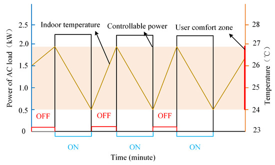
Figure 1.
The intermittent characteristic of AC.
It should be noted that the intermittent characteristics are more reflected in large-capacity single DSRs. When multiple DSRs are aggregated in frequency control, the effects of intermittent characteristics can be mitigated by suitable coordination and complement strategy. However, this does not mean that the aggregated DSRs does not have intermittent characteristics. Simple coordination and high demand for aggregated DSRs in a short-term time will also result in intermittent characteristics.
A traditional generator, i.e., a thermal and hydroelectric power generator, can provide a constant supply of power and therefore does not have intermittent characteristics [36]. For renewable energy generator, i.e., wind and photovoltaic generator, the intermittent characteristics are often discussed, and there are some differences from DSRs. The intermittent characteristics of renewable energy generators mainly come from the change of environment, which causes the uncertainty output power. We cannot control environment change, but we can actively control the frequency control time and adjustment capacity of DSRs.
Actually, the intermittent characteristics of DSRs have attracted the attention of some scholars in this field of research. They call the response time duration the maximum off time and which DSRs can provide power to response frequency deviation [37]. This characteristic is also referred to as a physical operation characteristic in some articles [18]. However, they rarely design control strategies specifically for this characteristic and evaluate the stability of the system.
When DSRs with intermittent characteristics participate in frequency control, the frequency regulation capacity provided by DSRs is similar to a controllable disturbance. This poses two problems for the power systems: First, this characteristic adds a nonlinear item to the power system and increases the risk of system instability. Besides, the generation-side control strategy needs to be coordinated and adjusted due to the addition of DSRs. Therefore, we need to find an appropriate control method for DSRs to ensure system stability.
2.2. Intermittent Control Method for Intermittent Characteristics of DSRs
In this paper, an intermittent control method is used to alleviate the problems caused by the intermittent characteristics of DSRs, and in this section, we introduce general intermittent control methods. The relationship between the intermittent control method and the intermittent characteristics of DSRs is also described.
It is assumed that DSRs participate in frequency control through primary frequency control, this means that DSRs autonomously monitors the frequency and responds to it. So the response power of DSRs for frequency control can be expressed as formula (1).
where is the response power of DSRs for frequency control, is the frequency deviation, is the intermittent gain in the intermittent control.
With the intermittent control method, we can express as formula (2).
where is a constant control gain, is the control period, and is called the control width.
The intermittent gain can simply describe the intermittent characteristics of DSRs. There are there unknown parameters K, T and , which need to be given according to intermittent characteristics of different DSRs. Among them, the gain K, like the droop gain, determines the response power of DSRs with unit frequency deviation. The control period T corresponds to the time when DSRs complete the whole process include turn on and off once. The control width depends on the response time duration (the time when DSRs are controllable) in one control period.
Therefore, this paper describes the intermittent characteristics of DSRs by formulas (1) and (2) based on the intermittent control method. The intermittent gain will be designed as the core of a DSRs controller. The control period T and control width depends more on the characteristics of the DSRs itself. Because the stability of the system should be considered when designing the DSR controller, the detailed design process and control parameters will be shown in Section 3.
2.3. Open-Loop LFC System Model
After the intermittent characteristics of DSRs are reflected by the intermittent control method, we need to consider how to add DSRs into the traditional LFC system. Refer to the traditional two-area LFC system in [1], which is shown in Figure 2.
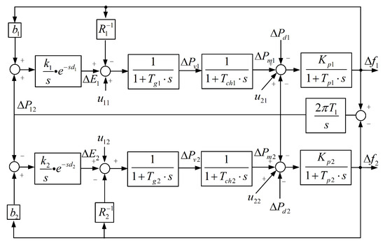
Figure 2.
Two-area LFC system model considering DSR.
In the two-area LFC system model described in Figure 2, are the frequency deviation, mechanical power deviation, electromagnetic power deviation, power change in secondary frequency control in area i. is the tie-line power deviation. represent control gain in secondary frequency control, time delay, governor time constant, turbine time constant, system gain, system time constant in area i. is the droop gain in primary frequency control in area i. is a constant.
The system dynamic state–space representation can be described by:
where the state vector is defined as . is the disturbance vector defined as . A and are system matrix, is the input matrix from generation-side resources, is the input matrix from DSRs. is the input matrix from random disturbance. C is the output matrix. is the direct transmission matrix. N is the number of area of the power systems, which is constant 2. Some specific values can be seen in Appendix A.
At this point, there are two control inputs that can help ensure the stability of the LFC system. The former control input represents extra primary frequency control from generation-side resources and the latter represents intermittent control from DSRs. The work of this paper designs the form of these control inputs.
In designing the controllers, the extra primary frequency control from generation-side resources can be expressed as:
where L is the feedback gain.
2.4. Closed-Loop LFC System Model and Robust Performance
By substituting and into Equation (3), the closed-loop state equation of the system can be obtained:
where L, K and are the controller gains and control width that need to be determined.
In order to ensure the robustness of the LFC system under different disturbance, the closed-loop LFC system (7) possess performance ; that is, the following holds:
under the initial conditon , where is a prescribed level.
3. Main Result
Considering the closed-loop LFC system, the most important problem is how to ensure the stability and meet the performance by designing the controllers’ parameters L, K and . This section first gives some common lemmas, and then analyzes the stability and robust performance of the system.
3.1. Preliminaries
Before the stability analysis of the system, some common theorems are also listed here.
Lemma 1.
For any vectors x, and positive-definite matrix , the following matrix inequality holds:
Lemma 2.
(Halanay inequality [38]) Let be a continuous function such that
is satisfied for . If , then
where , and is the smallest real root of the equation
Lemma 3.
[34]Let be a continuous function such that
is satisfied for . If , , then
where .
3.2. The Stability Analysis of the LFC System
For a LFC system, stability is a prerequisite. Using the lyapunov stability method, the stability analysis of the LFC system under intermittent control can refer to Theorem 1. For proof of the Theorem 1, refer to Appendix B.
Theorem 1.
The system is exponentially stable, if there exist positive symmetrical matrices , and and the matrix R, Y, intermittent control parameter T and δ, positive constants satisfying the following conditions:
- (a)
- (b)
- ,
- (c)
- ,
- (d)
- (e)
- (f)
- ,
where r is the positive solution of , , X satisfies , , . And the state feedback gains L and K can be constructed as and .
3.3. The Performance Analysis of the LFC System
In order to ensure the robustness of the LFC system under different disturbance, we must make the LFC system posses a performance.
Theorem 2.
For a prescribed attenuation level , the frequency of controlled power system is asymptotically stable and posses performance.
Proof.
In the following, consider the performance of system (7) under the initial zero condition. It can be verified that for any nonzero from the proof of Theorem 1, the following equality is easily obtained
where
and
where , □
4. Case Studies
In this section, the controller proved and analyzed in Section 3 will be used in a two-area LFC system. The system matrix and input matrix of the two-area LFC system are given in Appendix A. The detailed parameters of the simulation system are shown in Table 1.

Table 1.
Parameters of two-area LFC system.
4.1. The Open-Loop LFC System
Assume that the LFC system represented by formula (3) has no additional control inputs, including generation-side resources input and demand-side resources input . The open-loop LFC system is unstable under large disturbances.
The load is increased 1 p.u in area 1 as a large disturbance, and the frequency deviation of the two-area LFC system is illustrated in Figure 3. It can be seen that if there is a large disturbance in the open-loop LFC system, it is difficult to recover to a stable and safe state quickly. Meanwhile, the stability of area 2 will be indirectly affected by the large disturbance in area 1.
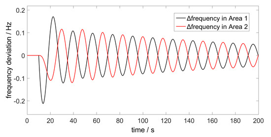
Figure 3.
Frequency deviation of the open-loop LFC system.
4.2. The Close-Loop LFC System
In this section, we designed two scenarios to demonstrate that the frequency deviation will be improved through reasonable coordinated control. The first scenario only uses the generation-side resources for frequency control. The second scenario uses both of the generation-side resources and DSRs.
In both scenarios, the proposed control method is solved by LMI. The detailed solving steps using LMI are shown in Figure 3.
4.2.1. Only Using Generation-Side Resources in LFC System
We only use generation-side resources to participate in the frequency control. We ignore the control from DSRs. So instead of solving formulae (a)–(f), we just need to solve formula (a). Meanwhile, the parameters K, in formula (a) are zero. This does not involve the nonlinear part, and the control parameter L can be directly solved:
The closed-loop LFC system is subject to the same disturbance as the open-loop LFC system. Under the generation-side control, the frequency variation of area 1 in the LFC system is shown in Figure 4. It can be seen that under the same disturbance, the dynamic frequency process of the LFC system has been significantly strengthened. The maximum frequency deviation of the system is also improved.
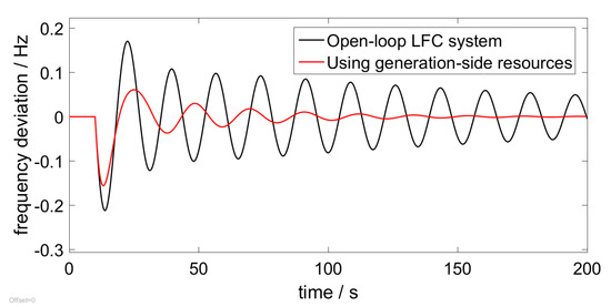
Figure 4.
Frequency deviation of area 1 under generation-side control.
4.2.2. Using DSRs and Generation-Side Resources in LFC System
We use the generation-side resources and DSRs to participate in frequency control. So we need to use LMI to solve equations (a)–(f) in Theorem 1. However, if we do not make any assumptions to solve equations (a)–(f), it is too hard to get the result. So we make some assumptions and attempts to simply this problem. The unknown values include the positive symmetrical , and and the matrix R, Y, intermittent control parameter T and , positive constants .
Through our analysis, we find that the system is too complex due to the higher dimensions, time delay and many unknown variables, and it is difficult to present a convex optimization state. So we try to make two assumptions which are realistic. These two assumptions are related to the intermittent characteristics of DSRs, as follows:
- As can be seen from Section 2.1 that parameters T and are affected by the intermittent characteristics of DSRs. In fact, these two parameters are fixed when the DSRs is identified. We can find some corresponding data from [7].
- For DSRs, when they participate in primary frequency control, they can only monitor the local frequency deviation of the system. They cannot obtain the other state such as the tie line power deviation andthe mechanical power deviation , etc. So parameter K should be a sparse matrix like the transposition of input matrix .
Then, the LMI program can be designed to solve the equation. The detailed design steps are shown in the Figure 5.
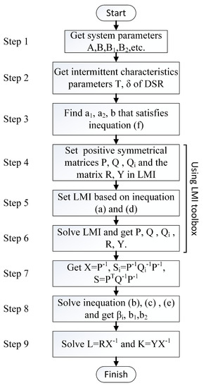
Figure 5.
The detailed solution process use LMI toolbox.
In Figure 5, step 2 and step 3 use the first assumptions, and step 4 uses the second assumptions when setting Y. The principle of selecting and in step 3 is: is as small as possible and is as large as possible. For different intermittent characteristics of DSR, different values K and L will be obtained. When T and take 10 s and 5 s, respectively, the parameters K and L can be solved.
We compared the effect of frequency control with only using generation-side control and additional using DSRs under different intermittent characteristic parameters . The relevant comparison results are shown in Figure 6. The corresponding power response of DSRs is shown in the Figure 7.
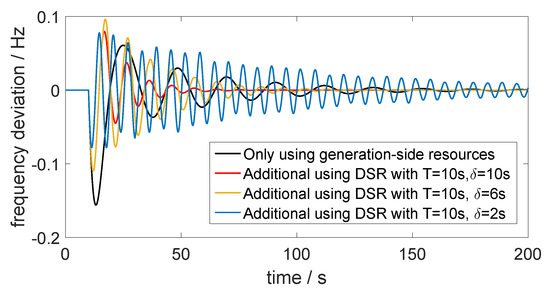
Figure 6.
Frequency deviation of area 1 under different intermittent control parameters.
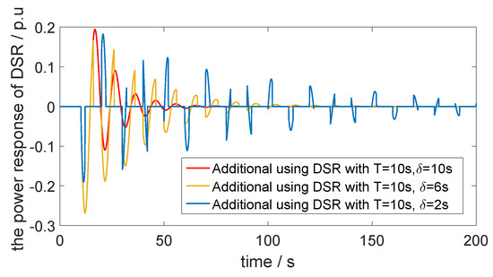
Figure 7.
The response power of DSRs under different intermittent control parameters.
As can be seen from Figure 6, when DSRs and generation-side resources participate in frequency control together, a better frequency control effect can be achieved than if generation-side resources control is used alone. However, because of the intermittent characteristic of DSRs, the intermittent control still has a certain influence on the LFC system. The more obvious the intermittent characteristics (the smaller the parameter is), the more significant influence will focus on the LFC system. At the same time, we can note that DSRs can improve the robustness of the LFC system, especially if the transient can ensure the grid frequency is kept within a safe range.
The power response of DSRs is shown in the Figure 7. We can see that DSRs are constantly turning up and off due to their intermittent characteristics. The more significant intermittent characteristics of DSRs, the frequency control rotation of DSRs will increase, and the corresponding time of DSRs participating in frequency control will be prolonged. In fact, we can reduce the rotation of DSRs by increasing the dead zone setting of DSRs.
Furthermore, in order to demonstrate the robustness of the proposed control design scheme, we further increased the disturbance in two areas , . The simulation results for area 1 and area 2 are provided in Figure 8 and Figure 9, where it can be found that the frequency could be maintained in a tolerable limit time. It can be found from these simulation results that the proposed intermittent control strategy is effective and useful.
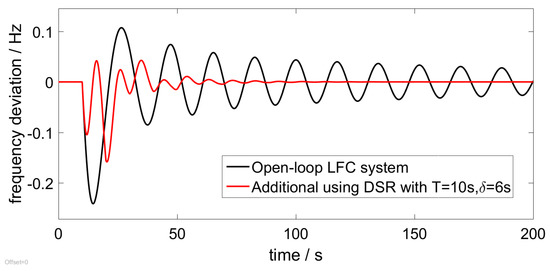
Figure 8.
Frequency deviation under open-loop and close-loop LFC system in area 1.
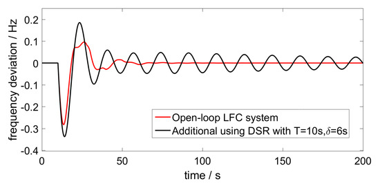
Figure 9.
Frequency deviation under open-loop and close-loop LFC system in area 2.
5. Conclusions
In this paper, the intermittent characteristic of DSRs is considered in a power system. An intermittent control strategy for this characteristic is designed. At the same time, the power generation-side resources and DSRs are used to build the cooperated LFC system, and the stability proof and performance analysis of this system are given. The summary is as follows.
- The intermittent characteristic of DSRs varies from user to user, which can affect the frequency performance of the power system.
- The intermittent control method can help the power grid adapt to the intermittent characteristics of DSRs.
- Reasonable coordination of generation-side resources and DSRs in frequency control can ensure the robustness of the LFC system and reduce the regulation pressure of the power generation-side.
Author Contributions
K.Y., Z.D., Y.L., M.H. and K.Z. in developing the ideas of this research. K.Y., Z.D. and K.Z. performed this research. All authors have read and agreed to the published version of the manuscript.
Funding
This work is supported by National Natural Science Foundation of China (No. 51977033), and State Grid Corporation of China Project “Research on Coordinated Technology for Dynamic Demand Response in Frequency Control“.
Conflicts of Interest
The authors declare no conflict of interest.
Appendix A
Appendix B
Proof of Theorem 1.
Consider the following Lyapunov function:
Calculate the derivative with respect to time t along the trajectory of error system (7), and estimate it.
For , using Lemma 1 and assumption, we have the following
Next, we prove that (A2) holds if (a)-(c) are satisfied. Let
Pre- and postmultiply to and apply the change of variables such that , , , . Then we can convert to:
For Schur complements, we can find is equivalent to the condition (a). By condition (a)–(c) and (A2), one has
Similarly, one has
Next, we will prove the closed loop system (7) with is exponentially stable.
By condition (a),(c),(d), one has
For , from conditions (b), (c) and (d), one has
where ,,.
Next, we will prove the error . From Lemma 2 and (A2), define
, one has
where r is the unique positive solution of .
From Lemma 3, one obtain the following
for .
Suppose that , then
Using mathematical induction, we can prove, for any positive integer n,
Assume Equation (A8) holds when . Now, we prove Equation (A8) is true when .
For any , there is , such that .
Let , one has the following inequality
Obviously,
□
References
- Sun, Y.; Wang, Y.; Wei, Z.; Sun, G.; Wu, X. Robust H∞ load frequency control of multi-area power system with time delay: A sliding mode control approach. IEEE/CAA J. Autom. Sin. 2017, 5, 610–617. [Google Scholar] [CrossRef]
- Bao, Y.Q.; Li, Y.; Hong, Y.Y.; Wang, B. Design of a hybrid hierarchical demand response control scheme for the frequency control. IET Gener. Transm. Distrib. 2015, 9, 2303–2310. [Google Scholar] [CrossRef]
- Ming, N.; Qian, C.; Manli, L.; Qi, W.; Yi, T. A Frequency Control Model for Cyber Physical Power System Considering Demand Response Strategy. Energy Procedia 2018, 145, 38–43. [Google Scholar] [CrossRef]
- Anwar, M.B.; Qazi, H.W.; Burke, D.J.; O’Malley, M. Harnessing the Flexibility of Demand-side Resources. IEEE Trans. Smart Grid 2018, 10, 4151–4163. [Google Scholar] [CrossRef]
- Cui, H.; Li, F.; Hu, Q.; Bai, L.; Fang, X. Day-ahead coordinated operation of utility-scale electricity and natural gas networks considering demand response based virtual power plants. Appl. Energy 2016, 176, 183–195. [Google Scholar] [CrossRef]
- Pourmousavi, S.A.; Nehrir, M.H. Real-time central demand response for primary frequency regulation in microgrids. IEEE Trans. Smart Grid 2012, 3, 1988–1996. [Google Scholar] [CrossRef]
- Molina-Garcia, A.; Bouffard, F.; Kirschen, D.S. Decentralized demand-side contribution to primary frequency control. IEEE Trans. Power Syst. 2010, 26, 411–419. [Google Scholar] [CrossRef]
- Molina-García, A.; Munoz-Benavente, I.; Hansen, A.D.; Gómez-Lázaro, E. Demand-side contribution to primary frequency control with wind farm auxiliary control. Trans. Power Syst. 2014, 29, 2391–2399. [Google Scholar] [CrossRef]
- Khooban, M.H.; Niknam, T.; Blaabjerg, F.; Dragičević, T. A new load frequency control strategy for micro-grids with considering electrical vehicles. Electr. Power Syst. Res. 2017, 143, 585–598. [Google Scholar] [CrossRef]
- Wang, Y.; Xu, Y.; Tang, Y. Distributed aggregation control of grid-interactive smart buildings for power system frequency support. Appl. Energy 2019, 251, 113371. [Google Scholar] [CrossRef]
- Zaman, M.; Bukhari, S.; Haider, R.; Hazazi, K.; Kim, C.; Ashraf, H. Demand Response Augmented Control with Load Restore Capabilities for Frequency Regulation of an RES-Integrated Power System. In Proceedings of the 2018 International Conference on Electrical Engineering (ICEE), Lahore, Pakistan, 15–16 February 2018; pp. 1–5. [Google Scholar]
- Samarakoon, K.; Ekanayake, J.; Jenkins, N. Investigation of domestic load control to provide primary frequency response using smart meters. IEEE Trans. Smart Grid 2011, 3, 282–292. [Google Scholar] [CrossRef]
- Delavari, A.; Kamwa, I. Sparse and resilient hierarchical direct load control for primary frequency response improvement and inter-area oscillations damping. IEEE Trans. Power Syst. 2018, 33, 5309–5318. [Google Scholar] [CrossRef]
- Shiltz, D.J.; Baros, S.; Cvetković, M.; Annaswamy, A.M. Integration of automatic generation control and demand response via a dynamic regulation market mechanism. IEEE Trans. Control Syst. Technol. 2017, 27, 631–646. [Google Scholar] [CrossRef]
- Fini, M.H.; Golshan, M.E.H. Frequency control using loads and generators capacity in power systems with a high penetration of renewables. Electr. Power Syst. Res. 2019, 166, 43–51. [Google Scholar] [CrossRef]
- Pourmousavi, S.A.; Nehrir, M.H. Introducing dynamic demand response in the LFC model. IEEE Trans. Power Syst. 2014, 29, 1562–1572. [Google Scholar] [CrossRef]
- Pourmousavi, S.A.; Behrangrad, M.; Nehrir, M.H.; Ardakani, A.J. LFC model for multi-area power systems considering dynamic demand response. In Proceedings of the 2016 IEEE/PES Transmission and Distribution Conference and Exposition (T&D), Dallas, TX, USA, 3–5 May 2016; pp. 1–5. [Google Scholar]
- Tang, Y.; Li, F.; Chen, Q.; Li, M.; Wang, Q.; Ni, M.; Chen, G. Frequency prediction method considering demand response aggregate characteristics and control effects. Appl. Energy 2018, 229, 936–944. [Google Scholar] [CrossRef]
- Xu, J.; Liao, S.; Sun, Y.; Ma, X.Y.; Gao, W.; Li, X.; Gu, J.; Dong, J.; Zhou, M. An isolated industrial power system driven by wind-coal power for aluminum productions: A case study of frequency control. IEEE Trans. Power Syst. 2014, 30, 471–483. [Google Scholar] [CrossRef]
- Kirchem, D.; Lynch, M.Á.; Bertsch, V.; Casey, E. Modelling demand response with process models and energy systems models: Potential applications for wastewater treatment within the energy-water nexus. Appl. Energy 2020, 260, 114321. [Google Scholar] [CrossRef]
- Han, S.; Han, S.; Sezaki, K. Development of an optimal vehicle-to-grid aggregator for frequency regulation. IEEE Trans. Smart Grid 2010, 1, 65–72. [Google Scholar]
- Abrishambaf, O.; Faria, P.; Vale, Z. Application of an optimization-based curtailment service provider in real-time simulation. Energy Inf. 2018, 1, 3. [Google Scholar] [CrossRef]
- Qazi, H.W.; Flynn, D. Synergetic frequency response from multiple flexible loads. Electr. Power Syst. Res. 2017, 145, 185–196. [Google Scholar] [CrossRef]
- Liu, H.; Huang, K.; Wang, N.; Qi, J.; Wu, Q.; Ma, S.; Li, C. Optimal dispatch for participation of electric vehicles in frequency regulation based on area control error and area regulation requirement. Appl. Energy 2019, 240, 46–55. [Google Scholar] [CrossRef]
- Muñoz-Benavente, I.; Hansen, A.D.; Gómez-Lázaro, E.; García-Sánchez, T.; Fernández-Guillamón, A.; Molina-García, Á. Impact of combined demand-response and wind power plant participation in frequency control for multi-area power systems. Energies 2019, 12, 1687. [Google Scholar] [CrossRef]
- Muñoz-Benavente, I.; Gómez-Lázaro, E.; García-Sánchez, T.; Vigueras-Rodríguez, A.; Molina-García, A. Implementation and assessment of a decentralized load frequency control: Application to power systems with high wind energy penetration. Energies 2017, 10, 151. [Google Scholar] [CrossRef]
- Loram, I.D.; Gollee, H.; Lakie, M.; Gawthrop, P.J. Human control of an inverted pendulum: is continuous control necessary? Is intermittent control effective? Is intermittent control physiological? J. Physiol. 2011, 589, 307–324. [Google Scholar] [CrossRef] [PubMed]
- Xia, W.; Cao, J. Pinning synchronization of delayed dynamical networks via periodically intermittent control. Chaos Interdisciplin. J. Nonlinear Sci. 2009, 19, 013120. [Google Scholar] [CrossRef]
- Ruan, S.; Filfil, R.S. Dynamics of a two-neuron system with discrete and distributed delays. Physica D Nonlinear Phenomena 2004, 191, 323–342. [Google Scholar] [CrossRef]
- Yuan, K.; Cao, J.; Li, H.X. Robust stability of switched Cohen–Grossberg neural networks with mixed time-varying delays. IEEE Trans. Syst. Man Cybern. Part B Cybern. 2006, 36, 1356–1363. [Google Scholar] [CrossRef]
- Żochowski, M. Intermittent dynamical control. Physica D Nonlinear Phenomena 2000, 145, 181–190. [Google Scholar] [CrossRef]
- Liu, Z.W.; Yu, X.; Guan, Z.H.; Hu, B.; Li, C. Pulse-modulated intermittent control in consensus of multiagent systems. IEEE Trans. Syst. Man Cybern. Syst. 2016, 47, 783–793. [Google Scholar] [CrossRef]
- Li, C.; Feng, G.; Liao, X. Stabilization of nonlinear systems via periodically intermittent control. IEEE Trans. Circuits Syst. Express Briefs 2007, 54, 1019–1023. [Google Scholar]
- Li, C.; Liao, X.; Huang, T. Exponential stabilization of chaotic systems with delay by periodically intermittent control. Chaos: Interdisciplin. J. Nonlinear Sci. 2007, 17, 013103. [Google Scholar] [CrossRef] [PubMed]
- Cao, J.; Yuan, K.; Ho, D.W.; Lam, J. Global point dissipativity of neural networks with mixed time-varying delays. Chaos Interdisciplin. J. Nonlinear Sci. 2006, 16, 013105. [Google Scholar] [CrossRef]
- Chen, C.; Zhang, K.; Yuan, K.; Zhu, L.; Qian, M. Novel detection scheme design considering cyber attacks on load frequency control. IEEE Trans. Ind. Inf. 2017, 14, 1932–1941. [Google Scholar] [CrossRef]
- Carvalho, J.P.; Shafie-khah, M.; Osório, G.; Rokrok, E.; Catalão, J.P. Multi-Agent System for Renewable Based Microgrid Restoration. In Proceedings of the 2018 International Conference on Smart Energy Systems and Technologies (SEST), Sevilla, Spain, 10–12 September 2018; pp. 1–6. [Google Scholar]
- Halanay, A. Differential Equations: Stability, Oscillations, Time Lags, 1st ed.; Academic Press: New York, NY, USA, 1966; pp. 611–615. [Google Scholar]


© 2020 by the authors. Licensee MDPI, Basel, Switzerland. This article is an open access article distributed under the terms and conditions of the Creative Commons Attribution (CC BY) license (http://creativecommons.org/licenses/by/4.0/).