People Walking Classification Using Automotive Radar

Abstract

Automotive radars are able to guarantee high performances at the expenses of a relatively low cost, and recently their application has been extended to several fields in addition to the original one. In this paper we consider the use of this kind of radars to discriminate different types of people’s movements in a real context. To this end, we exploit two different maps obtained from radar, that is, a spectrogram and a range-Doppler map. Through the application of dimensionality reduction methods, such as principal component analysis (PCA) and t-distributed stochastic neighbor embedding (t-SNE) algorithm, and the use of machine learning techniques we prove that is possible to classify with a very good precision people’s way of walking even employing commercial devices specifically designed for other purposes.

1. Introduction

Recognition of a person’s type of movement has implications for many aspects of daily life, from security applications to monitoring for assisted living. Discriminating whether a person is running or walking normally in airports or shopping centers, for example, may help video surveillance to detect possible dangerous situations [1,2,3]. Tools designed for this purpose involve the use of contactless devices, and radar technology is particularly suitable for the mentioned scenario.

Besides its ability to detect the presence of targets of all kinds, sometimes even at considerable distances, radar technology has attracted a large attention thanks to its versatility and usefulness in several fields, from medical applications [4] to traffic surveillance monitoring [5].

In this paper we consider the use of an automotive radar to classify different types of monitored actions. With respect to the work described in Reference [6], the examined activities present less evident differences, since our goal is to distinguish people’s way of walking on the basis of their speed. Moreover, the radar here considered works with a higher frequency range and therefore a smaller wavelength, thus allowing a better interaction with objects and improved performance in the micro-Doppler extraction. In addition, the millimeter wave technology exploited allows us to discriminate with a good accuracy also the position of the hands during the walk, whether they are in free movement or hold in pockets. Speed and hands movement classification is performed by using Principal Component Analysis (PCA) and t-distributed Stochastic Neighbor Embedding (t-SNE) methods for feature extraction and supervised learning for the classification task. Different algorithms have been tested, obtaining the best performance in terms of accuracy by using the Nearest Neighbor (NN) and the Support Vector Machine (SVM).

Related Work

Automotive radars with Frequency Modulated Continuous Wave (FMCW) transmission find many applications beyond their original purpose. Recent studies revealed how radars can be exploited to improve road safety and autonomous driving by recognizing the presence of pedestrians starting from micro-Doppler tracks, focusing in particular on the recognition of different parts of the human body [7,8,9], sometimes applying classification algorithms able to distinguish whether the detected target is a pedestrian or not with a very high accuracy [10]. Through the micro-Doppler components it is also possible to characterize a person’s movement or to identify a fall [11]. Moreover, micro-Doppler features have been often exploited in several aspects of human recognition, such as arm motion analysis [12], identification of target human motions [13], or to distinguish people walking in a noisy background [14]. Low power Frequency Modulated Continuous Wave (FMCW) radar and micro-Doppler tracks have been recently used with various scopes, such as discriminating armed from unarmed people [15], identifying people on the basis of their gait characteristics [16,17,18] or their movements [19], and for gestures recognition [20]. Moreover, radar technology has been successfully applied to the medical field [21,22], for example to remotely monitor the cardiac and respiratory frequency [23]. Principal Component Analysis (PCA) has been often exploited in radar applications, as an instrument to reduce the dimensionality of the available feature space and to automatize the feature extraction and selection procedure [24,25], together with deep learning algorithms for fall detection [26] and human activity recognition [27]. Recent works considered the application of deep learning techniques for gait classification, using smart sensors [28] and radar-based techniques [29] to discriminate aided from unaided motion.

From the year 2022 the 24 GHz bandwidth will no longer be available because of new regulations and ETSI and FCC standards, making it necessary to move towards other frequencies [30]. As regards radar applications, the only available bandwidth will be the ISM bandwidth that have only 250 MHz available, with a performance loss in distance. This explains the presence on the radar market of sensor for industrial and automotive applications working at frequencies over 76 GHz.

As an alternative to radar systems, different contactless technologies have been proposed for gait analysis and walking classification, based on the processing of video (RGB) or video+depth (RGBD) signals. Generally, the main purpose of these research activities is for medical purposes or related to safety issues. In Reference [31], a system able to perform an automatic detection and classification of gait impairments, based on the analysis of a single 2D video, is presented. The main drawback related to the use of video signal is related to privacy issues. To solve this problem, in Reference [32], a representation of gait appearance, with the aim of person identification and classification, is described, based on simple features such as moments extracted from orthogonal view video silhouettes of human walking motion. The availability of a low cost, marker-free, and portable device as Microsoft Kinect Camera allows to develop methods that can respond to the changes in the gait features during the swing stage, tracking the skeletal positional data of body joints to assess and evaluate the gait performance [33]. While being a low cost sensor, Microsoft Kinect is able to track human motion without using wearable sensors and with acceptable reliability. In Reference [34], the standard error of measurement and minimal detectable change sing Kinect is evaluated, confirming the validity of this sensor with standardized clinical tests in individuals with stroke.

The rest of the paper is organized as follows. Section 2 describes the radar used, along with the composition of the transmitted signals and the devices configuration. In Section 3 we outline the signal processing applied to extract spectrograms and maps from the data obtained. Section 4 the dimensionality reduction techniques and classification algorithms applied are introduced. Experimental results are shown in Section 5. Finally Section 6 concludes the paper.

2. Radar System Description

2.1. Used Devices

The radar used in this paper is the Texas Instruments AWR 1642 [35], originally developed for the automotive market [36]. Being designed for industrial applications, it has reduced costs with respect to other types of radar, and its use in the context of interest of this work allows to verify if it is possible to classify people movements with a good accuracy also exploiting commercial devices. It exploits two bandwidths, in the frequency ranges of 76–77 GHz and 77–81 GHz with 1 and 4 GHz bandwidth, respectively. The former is used for long range applications (up to 150 metres) and the latter for short range applications (up to 30 metres). The radar considered in Reference [6] is an Ankortek SDR-Kit 2400AD, a Software Defined Radio (SDR) working in the frequency range 24–26 GHz, with a maximum bandwidth of 2 GHz and a chirp time and maximum ramp slope of 15.625 MHz/$\mathsf{\mu }$s [37]. With respect to radar used in Reference [6], the higher frequency, the larger bandwidth and the steeper ramp allow to achieve an increase of twenty time in range performance and three times in speed.

An additional characteristic of AWR 1642 is the presence of multiple-input multiple output (MIMO) technology in the sensor [38], which, in case of radar systems, has the goal of improving performance in angular detection.

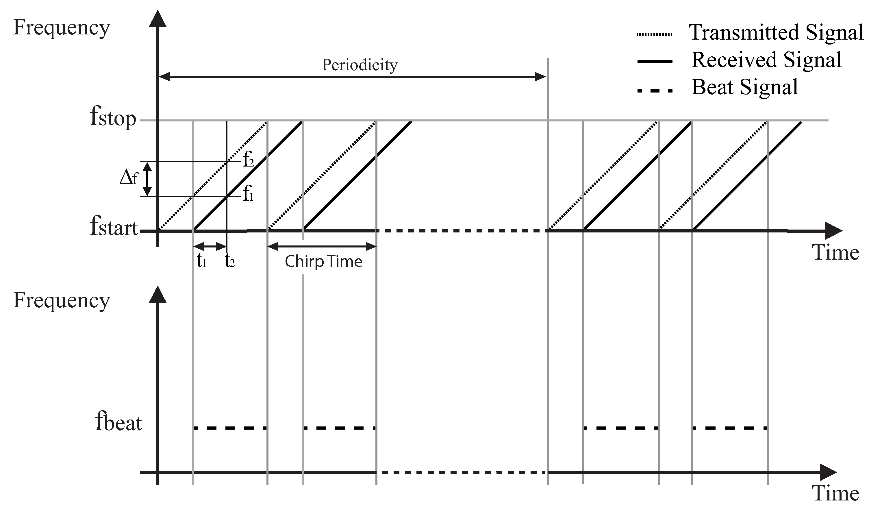
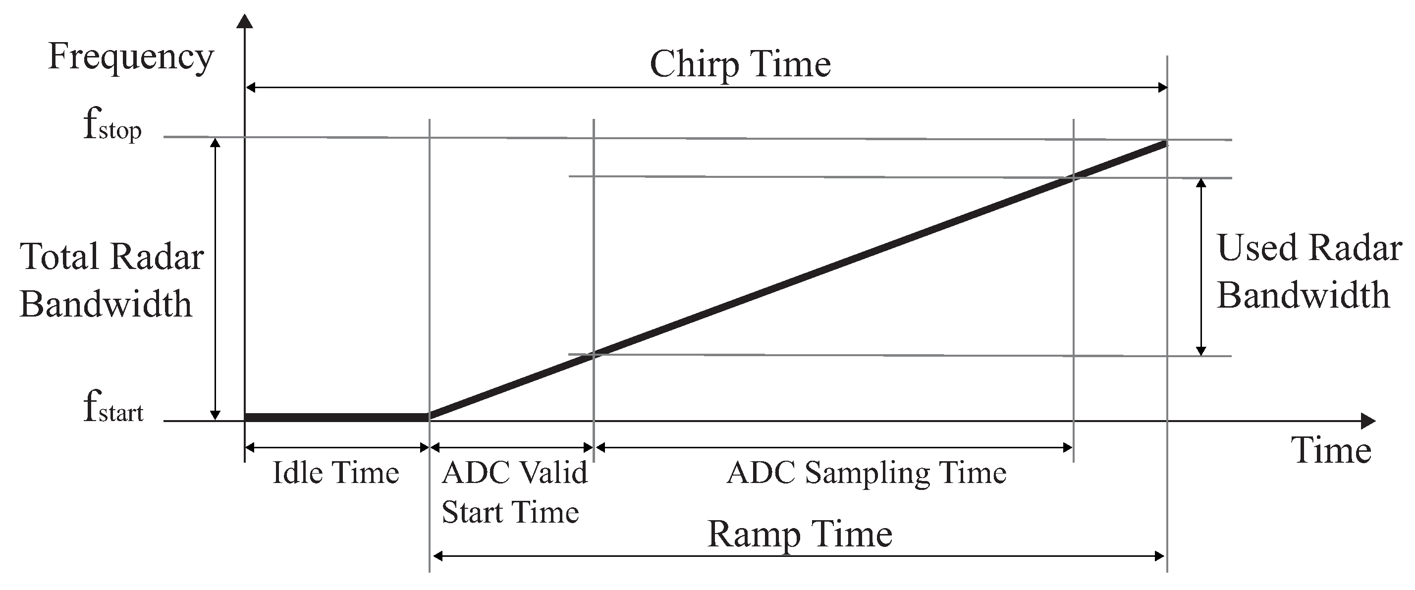
2.2. Transmitted Signals

Signals are transmitted using Frequency Modulated Continuous Wave (FMCW) modulation, this requires that the transmission frequency varies linearly from a minimum value to a maximum value in a time interval, called chirp time. The transmitted chirps are grouped into frames. Inside each frame, which has a time duration called periodicity, the radar transmits a certain number of chirps, as schematized in Figure 1.

Each chirp is built as shown in Figure 2. We have an Idle Time, needed because the ramp generator requires some time to restart the ramp and generate a new chirp. Then a guard time, or analog-to-digital converter (ADC) Valid Start Time, is considered in the first part of the ramp, which is not linear and may lead to a performance reduction, as described in Reference [39].

Then we have the effective ADC Sampling Time, which represents the time duration of the ramp acquired by the radar. Within this interval analog-to-digital converters (ADCs) samples of the IF signals are collected. As easily observable in Figure 2, a time shorter than the total ramp time $t_{ramp}$ is used, so the used radar bandwidth B is smaller than the maximum possible $TB$, and is calculated as

$$B=AD{C}_{SamplingTime}·S\le TB=t_{ramp}·S,$$

(1)

where S represents the slope of the ramp and $AD{C}_{SamplingTime}$ is given by the product between the the number of samples $n_{samples}$ acquired for each chirp and the sampling period $t_{sampling}$. The devices configuration must take in account these parameters in order to avoid as much as possible the non linear effects of the sensor.

The importance of avoiding the first part of the ramp is evident from the analysis of the intermediate frequency (IF) signal during time and on the complex plane. As briefly described in Reference [40], it is possible to see this effect on the IQ plot. Using different calibrations, the first with analog-to-digital converter (ADC) Valid Start Time equal to zero, and the second with time equal to 6 $\mathsf{\mu }s$ it is possible to observe how this imperfection can be avoided without the need of using an algorithm. Figure 3a shows 500 samples of IF signal across two different chirps. If the guard time is not used, there is a spike at the beginning of the first chirp. In Figure 3b the case of the same segment of IF signal, with an analog-to-digital converter (ADC) Valid Start Time of 6 $\mathsf{\mu }s$ is depicted, not showing the same effect. The spike disappears with a minimum value of 3 $\mathsf{\mu }s$.

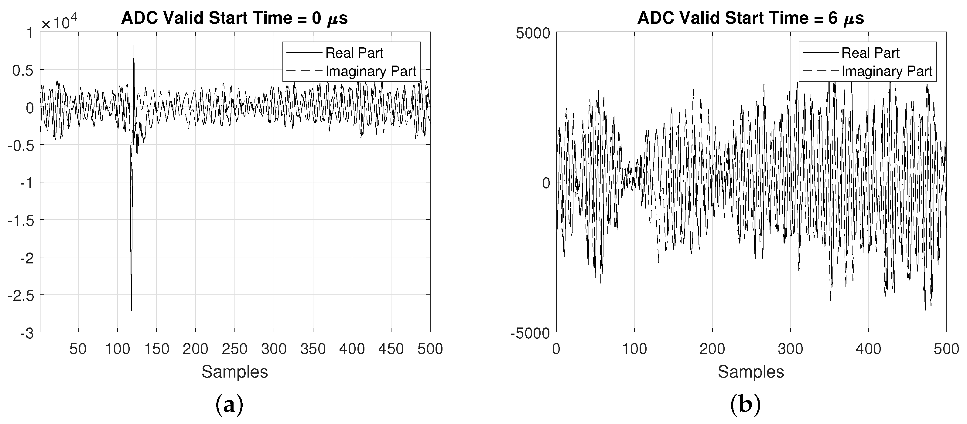
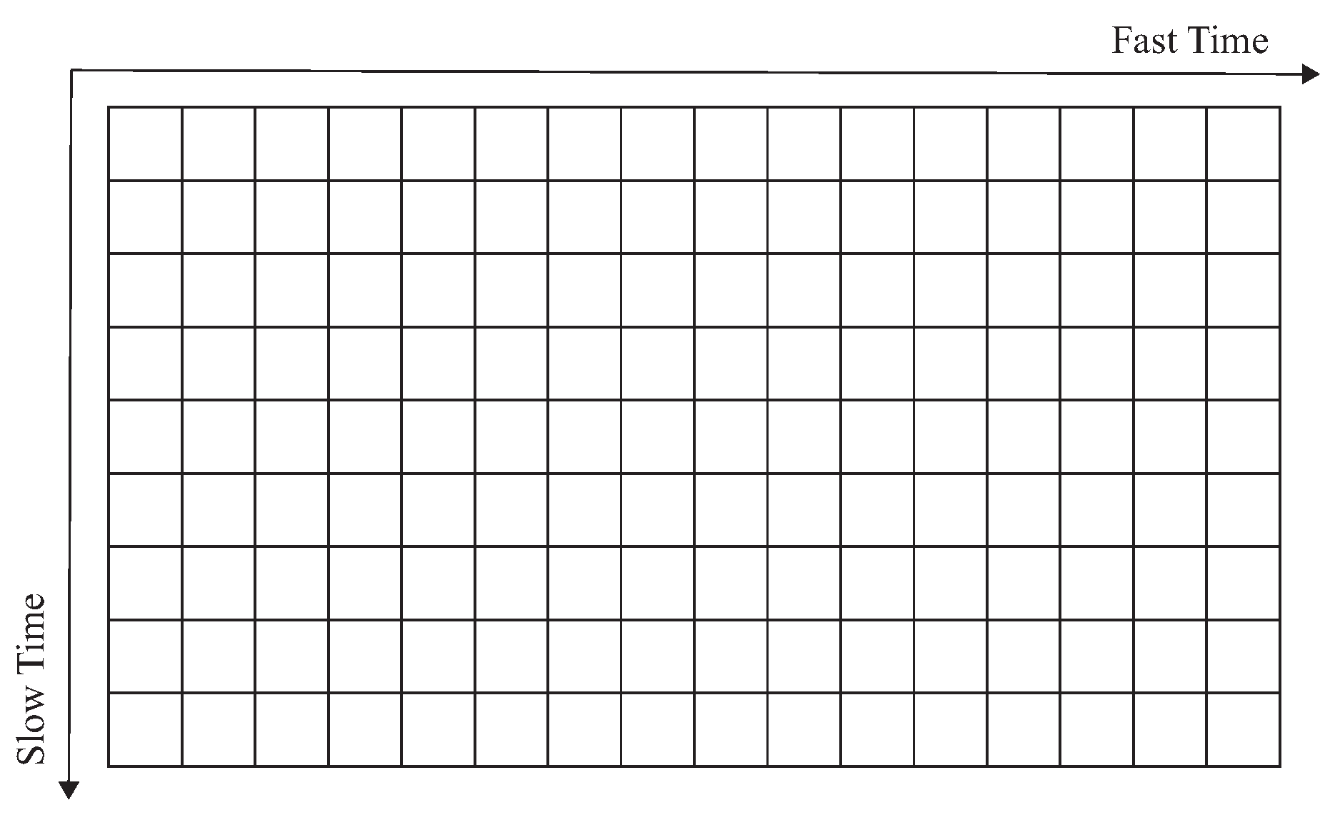
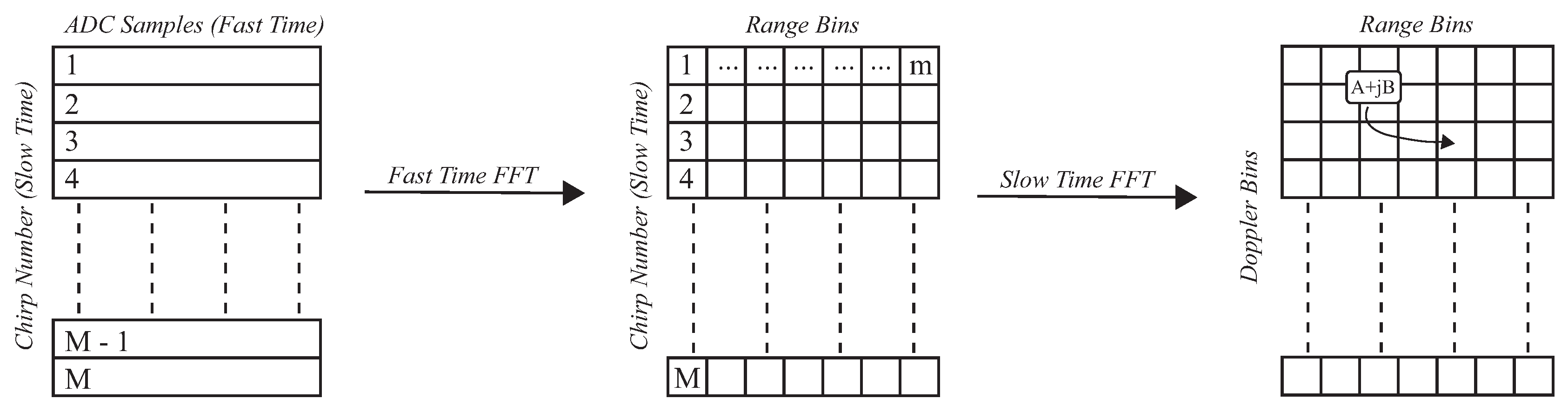
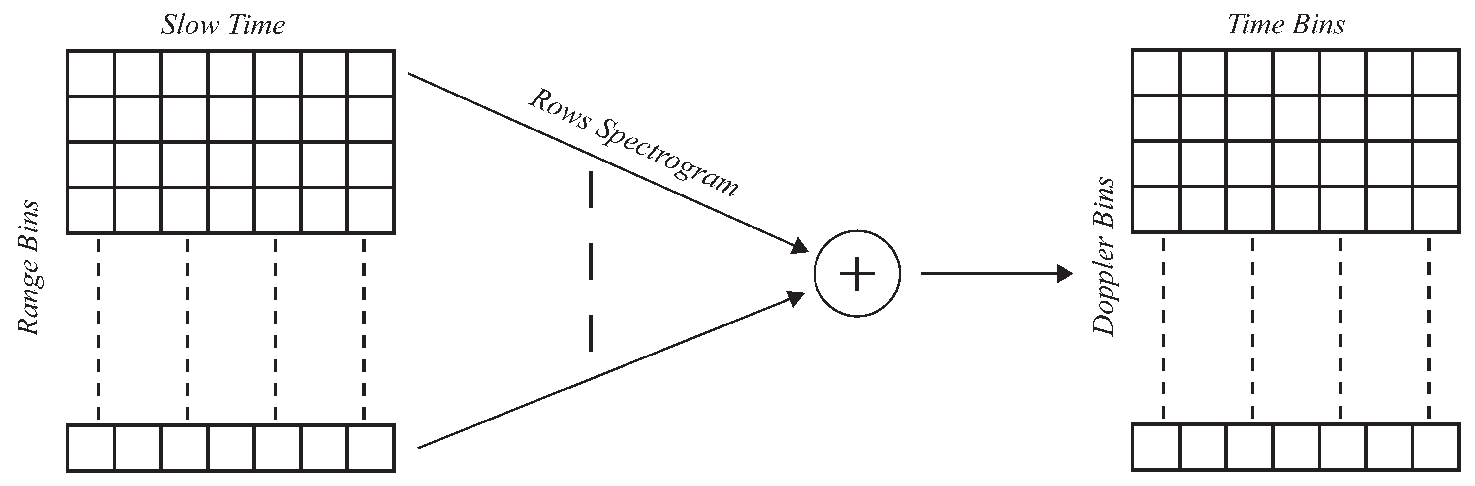
3. Radar Signal Processing

On the basis of the used configuration we have four available receiving lines. To perform our analysis we need just one of them, so we can sum the complex samples coming from the analog-to-digital converters in order to improve the signal-to-noise ratio. We thus obtain a vector of complex samples which can be reorganized in the form of matrix, as shown in Figure 4. Along the rows of the matrix, also called fast time, we have samples from single chirps, while on the columns, or slow time, we samples from different chirps.

From this raw matrix we can extract two types of map to classify different types of movement. The first one contains information about distance and speed of the subject and it is obtained by applying a Fourier transform to columns and then to rows; this map is defined as Range-Doppler Map. Each element of the map is a complex number and it is built considering the total acquisition, as shown in Figure 5. Besides distance and speed, this allows to extract also the micro-Doppler components characterizing the movement.

Since our subjects are moving during the acquisitions, we can extract the spectrogram from each Range bin and hence characterize their micro-Dopplers along the entire activity.

During each acquisition all the objects are stationary with the exception of the subject under exam, therefore the only significant micro-Doppler components are related to her/him. The presence of stationary objects does not influence either the Range-Doppler map, but only the zero Doppler. As described in Reference [19], from this map is possible to identify the kind of movement carried out by the subject.

The second type of map can be extracted through spectrograms and is denoted as Doppler-Time Map. A spectrogram is the most common time-frequency representation [41], and it is derived from the Short Time Fourier Transform (STFT) according to the following equation

$${STFT}_x[k,n]=\sum _{r=-\infty }^{+\infty }x\left[r\right]w[n-r]e^{-j2\pi rk/N},k=0,1,\cdots ,N-1,$$

(2)

where n represents a discrete index of time, k is a discrete index of frequency and $w[·]$ is a window function. The Short Time Fourier Transform (STFT) can in fact be considered as the Fourier transform of a signal multiplied by a window sliding over time. A trade-off between resolution in time and in frequency must be found, and overlapping frequencies can help in this sense [42].

Starting from the range matrix, the second matrix in Figure 5, and applying the Short Time Fourier Transform (STFT) along the rows, we obtain the Doppler-Time map. This function uses windows of 512 samples, with an overlap of 98% and an Hann window is applied. Figure 6 depicts this process.

By using both the mentioned maps it is possible to classify different kinds of movements, as will be explained in the next section.

4. Movements Classification

In this section we briefly describe the dimensionality reduction techniques and the classification algorithms used in the following section to discriminate the kinds of activities under consideration. As regards features extraction, we resort to two different methods to reduce data dimensionality, the Principal Component Analysis (PCA) and the t-distributed Stochastic Neighbor Embedding (t-SNE).

Both the maps obtained through the radar signal processing, that is, the Range-Doppler map and Time-Doppler map, are considered as images. Vectors resulting from the application of dimensionality reduction techniques to these images, that is, the principal components extracted from Principal Component Analysis (PCA) and the main dimensions given by the t-distributed Stochastic Neighbor Embedding (t-SNE), will serve as features vectors. We have a set of N images $I_n$ of dimension $[l\times m]$, with $n=1,\cdots ,N$. Images are initially vectorized row-wise and grouped in order to form a training set $\mathbf{X}={[x^{\left(1\right)},\cdots ,x^{\left(N\right)}]}^T$, where T denotes the transpose operator; rows of $\mathbf{X}$ correspond to observations and columns correspond to variables.

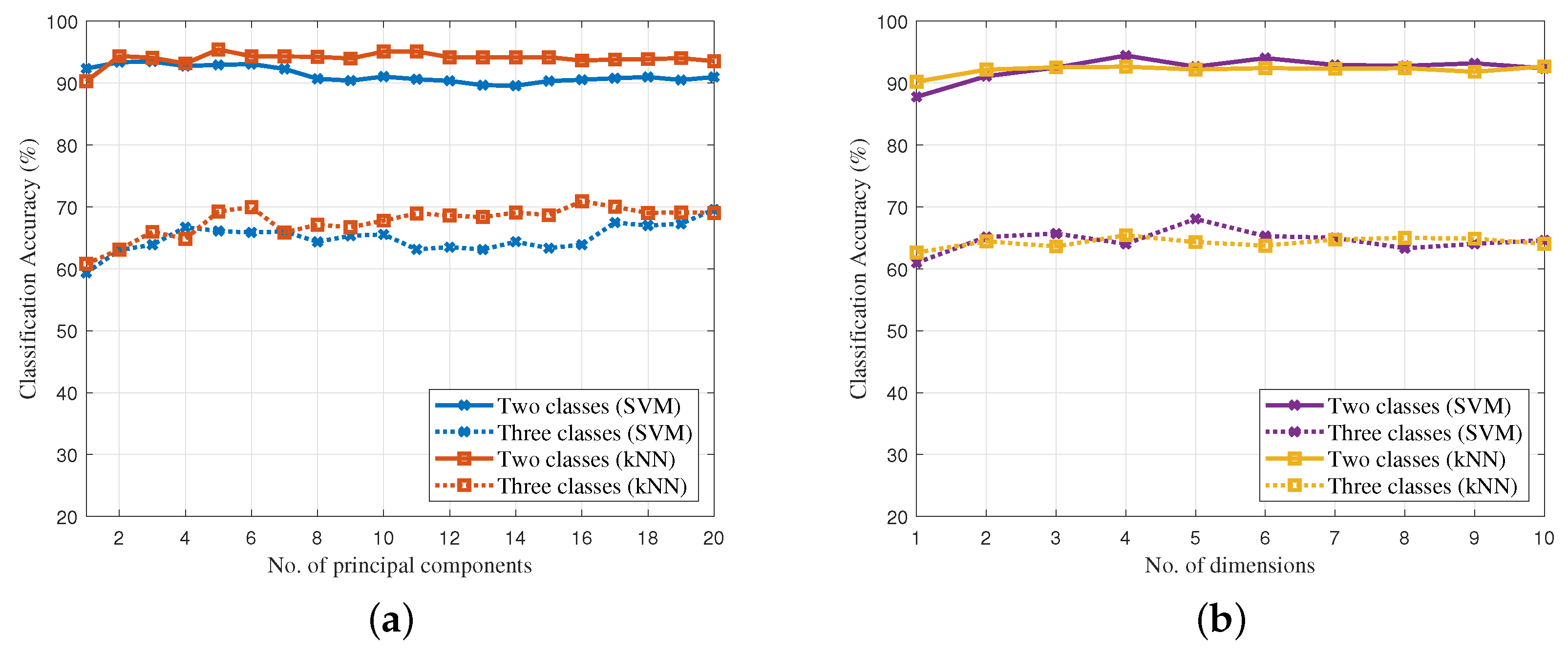
4.1. Principal Component Analysis

Principal Component Analysis (PCA) [43] is a non supervised transform also known as Karhunen-Loeve transform (KLT). It aims at finding suitable linear transformations y of the observed variables that are easily interpreted and capable of highlighting and summarizing the information inherent in the initial matrix I. This tool is especially useful when dealing with a considerable number of variables from which you want to extract the greatest possible information while working with a smaller set of variables.

Principal Component Analysis (PCA) can hence be described as a transformation of a given set of N vectors into inputs (variables) of the same length K placed in a vector N-dimensional $\mathbf{X}$, which allows to transform this vector into a second vector y, built in such a way that the first element of y includes the greatest possible variability (and therefore more information) of the original variables, that the second represents the greater variability of the $x_i$ after the first component, and so up to $y^{\left(N\right)}$ which takes into account the smallest fraction of the original variance. Therefore the main components are those linear combinations of the random variables $x^{\left(N\right)}$ according to the unit norm which make the variance maximum and which are uncorrelated.

The resulting vector y form the feature vector which can be used for classification. Moreover, Principal Component Analysis (PCA) algorithm is invertible, so original data can be easily recovered.

4.2. t-distributed Stochastic Neighbor Embedding

t-distributed Stochastic Neighbor Embedding (t-SNE) [44] is a non linear and non supervised transform, specifically designed to reduce dimensionality to 2 or 3 dimensions in order to display multidimensional data.

The t-distributed Stochastic Neighbor Embedding (t-SNE) algorithm consists of two main steps. Given our set of N vectorized images $x^{\left(1\right)},\cdots ,x^{\left(N\right)}$ with length $l·m$, t-SNE first computes the conditional probability $p_{j|i}$, which represents the similarity of datapoint $x_j$ to datapoint $x_i$. In other words, it evaluates the probability that $x_i$ would pick $x_j$ as its neighbor if neighbors were picked in proportion to their probability density under a Gaussian centered at $x_i$. In formulas,

$$p_{j|i}=\frac{exp(-\parallel x_i-x_j{\parallel }^2/2{\sigma }_i^2)}{{\sum }_{k\ne i}exp(-\parallel x_i-x_j{\parallel }^2/2{\sigma }_i^2)}.$$

(3)

t-distributed Stochastic Neighbor Embedding (t-SNE) then defines a similar probability distribution over the points in the low-dimensional map, and it minimizes the Kullback-Leibler (KL) divergence between the two distributions with respect to the locations of the points in the map.

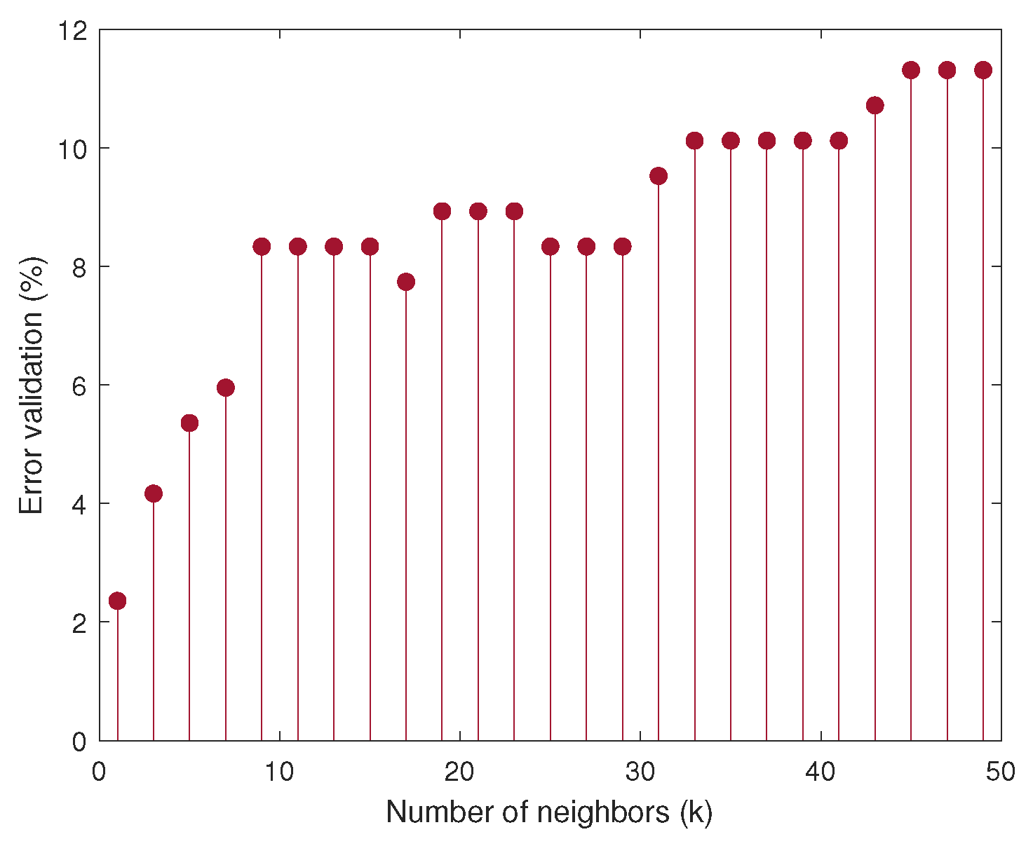
4.3. Classification Algorithms

As regards the classification task, we consider the use of k-Nearest Neighbor (NN) and Support Vector Machines (SVMs). They are both supervised and non parametric algorithms.

k-Nearest Neighbor (NN) is an instance-based algorithm, meaning that it does not explicitly learn a model. Instead, it chooses to memorize the training instances which are subsequently used as “knowledge” for the forecasting phase. In concrete terms, this means that only when a query is made in the database (i.e., when asked to provide a label with an input), the algorithm will use the training instances to send a response. As a drawback, this algorithm presents both a storage cost during the training phase, since it is necessary to store a potentially huge dataset, and a computational cost during the prediction phase since the classification of a given observation requires the vision and/or analysis of the entire dataset. In the context of classification, the k-Nearest Neighbor (NN) algorithm essentially boils down to determine a majority vote among the k closest neighbors to a given unknown instance. The proximity is defined by a distance metric, usually the Euclidean distance, between two data points.

Support Vector Machine (SVM) algorithm classifies data by creating a linear of non-linear decision boundary to separate different classes. It projects the data through a non-linear function to a space with a higher dimension, lifting them from their original space to a feature space, which can be of unlimited dimension. To perform this operation, Support Vector Machine (SVM) makes use of kernels, among which one of the most used is the Gaussian kernel.

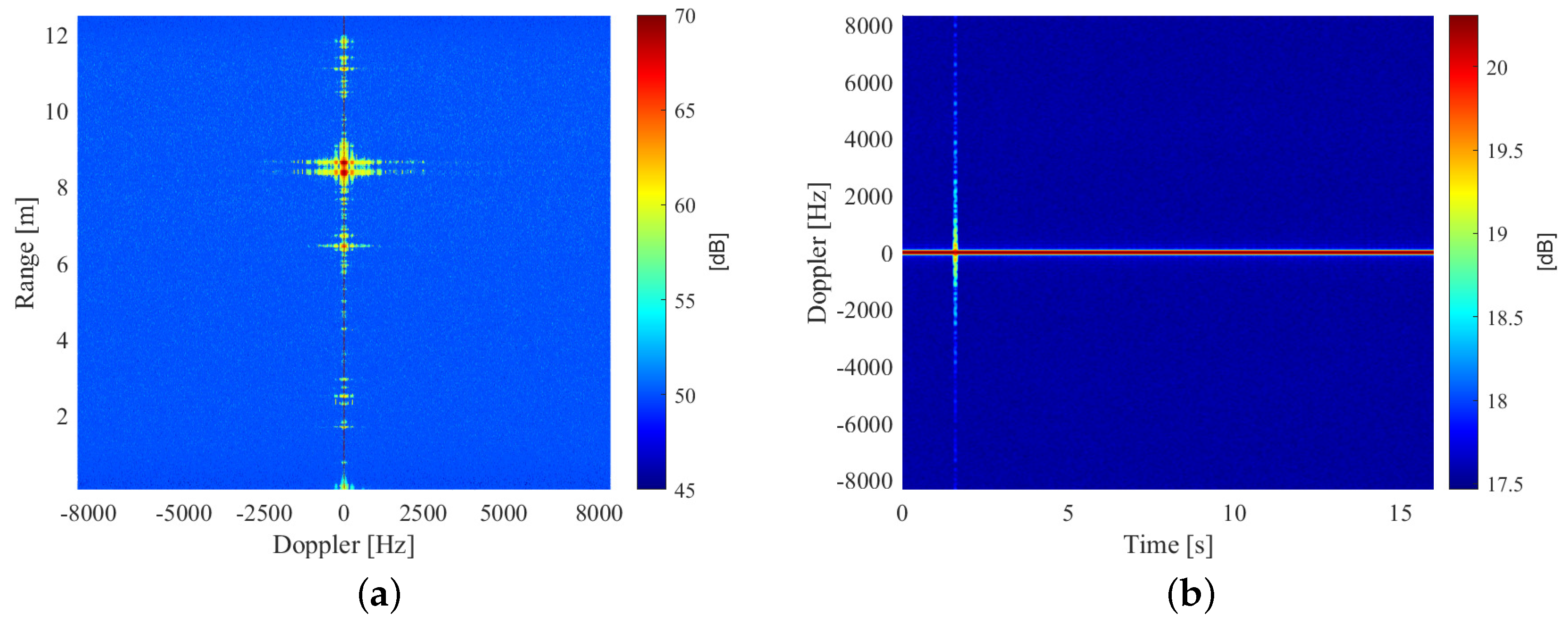
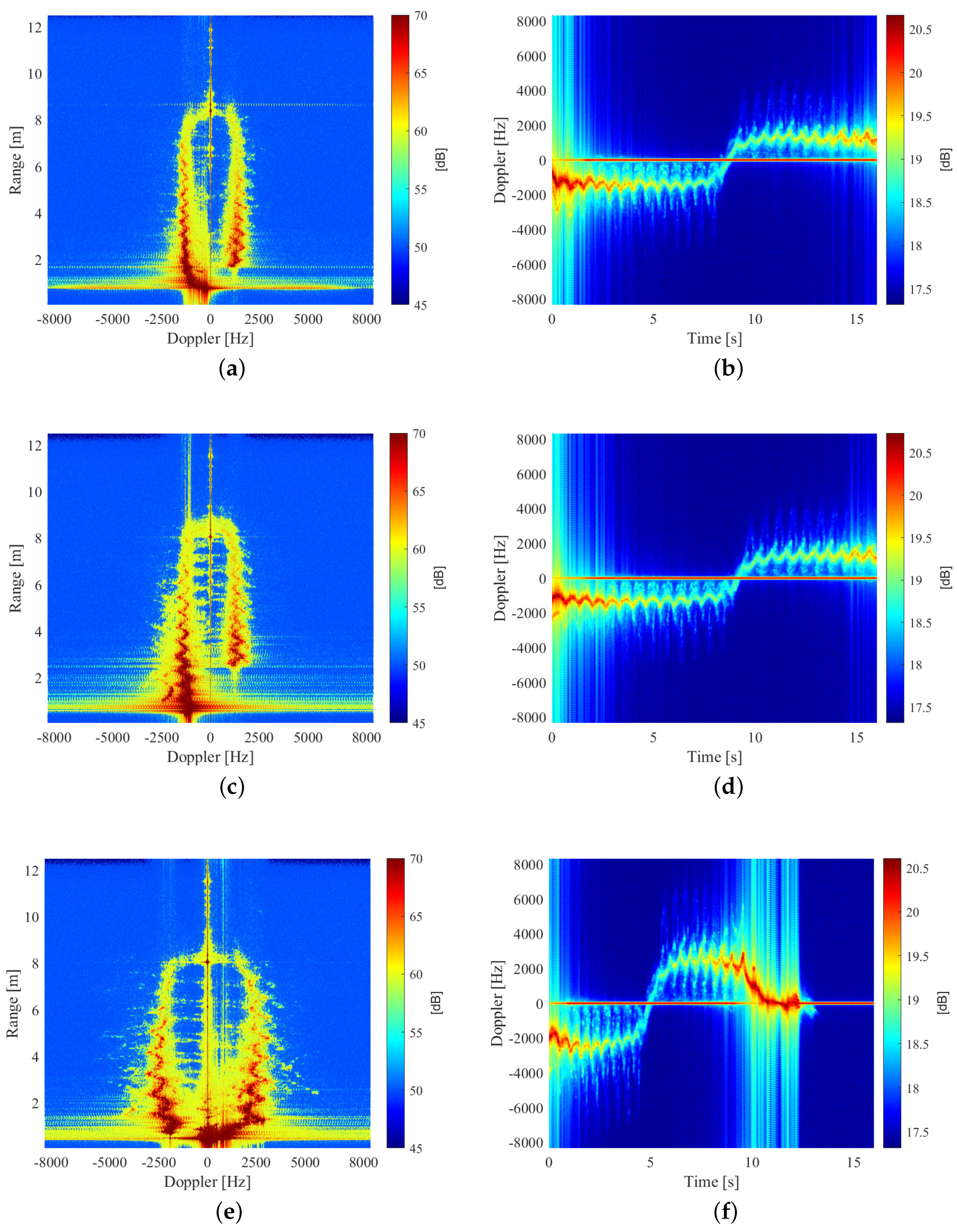
5. Experimental Results

5.1. Experimental Setup

In our experiments we consider a data set composed by nineteen subjects who repeated each activity for three times, for a total of 168 different acquisitions. Three different activities were examined:

• Slow walk;
• Fast walk;
• Slow walk with hands in pockets.

Note that we do not consider a data set built ad hoc: each subject was simply asked to walk in a “slow” or in a “fast” way, without specifying the number of steps or the time required to complete the activity, in order to generate data as realistic as possible. In addition acquisitions belonging to subjects of different height and weight were collected to provide a set comprehensive of a large variety of characteristics. Walking speed difference is subtle and depends on the person examined, who interpreted it subjectively. In general, the average speed measured for the fast walk is around 2 m/s, while for the slow walk, with both free hands or hands in pockets is about 1.2 m/s. Differences in subjects’ speed, including the “holding the arm” case (which is similar to our “hands in pockets”), have been considered in References [45,46], although their datasets were composed by 8 and 3 subjects, respectively.

The radar configuration parameters are chosen according to the measurement area selected and to the kind of activity required to the subjects. Some parameters are chosen according to the following range R equation

$$R=\frac{f_{beat}·c}{2·S},$$

(4)

where $f_{beat}$ is the beat frequency and c is the speed of light. We can evaluate the maximum speed of the target as

$$v_{target}=\frac{\lambda }{4·t_{chirp}},$$

(5)

where $\lambda$ represents the wavelength of the transmitted signal and $t_{chirp}$ is the time duration of the chirp. The measurement area is an hallway, about 12 meters long, and is free of furniture. During each activity the subject goes from the starting point in front of the RADAR to a distance of about 9 meters, and then comes back. Due the fact that the measurement time is of 16 seconds, it is possible that the acquisition ends before the subject returns to the initial position. The parameters used for the measurements are reported in

Table 1. RADAR parameters.

Parameter	Value
$f_{start}$	77 GHz
S	60.012 MHz/$\mathsf{\mu }s$
$t_{idle}$	100 $\mathsf{\mu }s$
ADC Valid Start Time	6 $\mathsf{\mu }s$
$f_s$	10 Msps
$t_{ramp}$	60 $\mathsf{\mu }s$
$n_{samples}$	512
$n_{frame}$	400
no. of chirps per frame	128
Periodicity	40 ms
Used Radar Bandwidth	3.6 GHz

.

A first analysis has been made on the background without any subject, which is depicted in Figure 7. Only one measurement has been performed, since the test area is the same for all the subjects. From this analysis is possible to see that the background does not affect the measurements, thus we can neglect its effect in the movements classification.

In Figure 8 we show an example a subject walking in different ways, displaying both Range-Doppler maps (on the left) and Doppler-time maps (on the right). It is possible to observe that slow and fast walk are easily recognizable in the maps. As expected, maps related to slow walk with hands in pockets present a slightly less evident Doppler with respect to free hands, but this effect is scarcely noticeable.

5.2. Classification

Data obtained after the processing of the radar signal are treated as images. Since their original size cannot be easily handled, all matrices have been reshaped to the same dimension $[195\times 119]$. In order to further reduce dimensionality and to extract features from images, Principal Component Analysis (PCA) and t-distributed Stochastic Neighbor Embedding (t-SNE) algorithm have been then applied separately to data.

In Figure 9a,b we show the classification accuracy resulting from exploiting a different number of principal components, by using a Nearest Neighbor (NN) classifier and a Support Vector Machine (SVM) algorithm. We choose to use a Gaussian kernel for the Support Vector Machine (SVM).The value of k for the k-Nearest Neighbor (NN) and the kernel used for Support Vector Machine (SVM) have been chosen by using a leave-one-out cross-validation algorithm, which aims at minimizing the validation error. Each sample of the dataset is alternatively selected as a validation set, whilst the remaining part represents the training set. In this way all samples are used only one time both for training, both for validation. Results obtained by the algorithm for odd values of k between 1 and 49 are shown in Figure 10, where k equal to 1 leads to an error of about 2.4%. The validation error obtained by different kernels in percentage is reported in

Table 2. Results of the leave-one-out cross validation for support vector machine (SVM) with different kernels.

Kernel	Linear	Gaussian	Polynomial
Error validation (%)	4.46	17.26	33.33

, thus directing the choice to the use of linear kernel in our scenario.

Sixty percent of the acquisitions are used for training, while the remainder is used for testing. Results have been averaged over 100 classification results obtained choosing training and test sets at random. We consider here only two classes, corresponding to the slow and fast walk. Interestingly, it is possible to observe that the number of principal components (or number of dimension in case of t-distributed Stochastic Neighbor Embedding (t-SNE) ) that here corresponds to the number of features, has a small impact on the classification performance. The application of Principal Component Analysis (PCA) or t-distributed Stochastic Neighbor Embedding (t-SNE) algorithm to extract features from images leads to very similar results, although t-distributed Stochastic Neighbor Embedding (t-SNE) was originally designed to reduce data to two or three dimensions, and becomes very slow for higher values. In addition, we obtain the same results using both Range-Doppler and Doppler-Time maps.

In

Table 3. Confusion matrix obtained applying SVM and kNN (into parentheses) on two classes, considering 5 principal components, $acc=93.5\%$.

True/Predicted	S	F
Slow Walk (S)	110 (109)	2 (3)
Fast Walk (F)	9 (8)	47 (48)

and

Table 4. Confusion matrix obtained applying SVM and kNN (into parentheses) on three different classes, considering 9 principal components, $ac{c}_{\mathrm{SVM}}=72\%$, $ac{c}_{\mathrm{KNN}}=66.7\%$.

True/Predicted	S	F	SH
Slow Walk (S)	33 (32)	2 (1)	21 (23)
Fast Walk (F)	4 (5)	49 (48)	3 (3)
Slow Walk with Hands in Pockets (SH)	16 (22)	1 (2)	39 (32)

we show the confusion matrices obtained by applying classification on two and three different classes. In the first table, measurements of slow walk and slow walk with hands in pockets have been incorporated into a single class, while in the second table they have been split into two separate classes. As predictable, distinguishing free hands from hands in pockets is a much more complicated task than identify different ways of walking. In the first case in fact the best accuracy obtained is about $72\%$ and red boxes highlight the presence of a number of misclassified examples, although the fast walk is recognized from the other activities with a high precision (87.5%); SVM methods seem to achieve better performance than KNN algorithms. In the latter case we have instead an excellent accuracy of more than $93\%$. In both Table 3 and Table 4 we highlighted a high presence of correct detections in green, while a high number of misclassified samples is marked in red.

In

Table 5. Comparison of different radar based methods for human walking classification.

	Radar Type	No. of Activities	Dataset Dimension	Algorithm	Best Accuracy
[*]	FMCW mmWave	2	19 subjects, 168 acquisitions	PCA/t-SNE + k-NN/SVM	93.5%
[*]	FMCW mmWave	3	19 subjects, 168 acquisitions	PCA/t-SNE + k-NN/SVM	72%
[45]	Ultra Wide Band	7	8 subjects, 280 acquisitions	PCA + SVM	89.1%
[46]	FMCW mmWave	5	3 subjects, 95 acquisitions	CV/TV + SVM	91%

, we give an overview of the results obtained by other works focused on the classification of walking activities through radar measurements, showing the best accuracies achieved. [*] denotes the present work. In Reference [45] 7 types of activities are considered, that is, walking backwards, limping, depressed, elderly, excited, holding the arm and walking in a zigzag, and the radar used is an Ultra-Wide Band; Reference [46] considers a Frequency Modulated Continuous Wave (FMCW) radar, and the examined activities are crawl, creep on hands and knees, walk, jog and run. Although the difference between walking slowly or quickly is less evident than the other activities, we prove that our system is able to achieve a better accuracy. Moreover, we consider a larger number of subjects that move differently from each other, thus confirming the validity of our method in a realistic context. The activity of holding the arm while walking [45], which is in some way comparable to our case of walking slowly with hands in pockets, could not be differentiated from the others at all, with a specific accuracy of 42.42% (see Reference [45], Table 2).

The subjectivity and the personal speed interpretation of the conducted tests represents the major error source for our classification model. A standardized time or number of steps during the experiment should probably improve the system performance, but this would not represent a realistic scenario and it is out of the scope of this work.

6. Conclusions and Future Works

We have assessed the performance of an automotive radar to classify different types of movements, focusing our attention to the distinction of people’s way of walking. The dataset was not built ad hoc, but we have collected acquisitions of subjects with different characteristics free to walk in a given indoor environment. We have considered the use of PCA and t-SNE techniques to reduce data dimensionality and to extract features, and then we have applied different classification algorithms. From the obtained results it is possible to state that movement classification of human targets is a much more complex task with respect to the discrimination of people from other objects. However, we have shown that, by exploiting the micro-Doppler components of the radar signal, we are able to identify with a high accuracy slow and fast walking. We have also characterized the presence or absence of movement of the arms with more than 72% of precision, which represents a good starting point for a future work. A possible future direction may also include the investigation of deep learning methods in our scenario in order to better distinguish small movements.

References

1. Frazier, L.M. MDR for law enforcement [motion detector radar]. IEEE Potentials 1998, 16, 23–26. [Google Scholar] [CrossRef]
2. Mazel, D.S.; Barry, A. Mobile Ravin: Intrusion Detection and Tracking with Organic Airport Radar and Video Systems. In Proceedings of the 40th Annual 2006 International Carnahan Conference on Security Technology, Lexington, KY, USA, 16–19 October 2006; pp. 30–33. [Google Scholar] [CrossRef]
3. Zyczkowski, M.; Palka, N.; Trzcinski, T.; Dulski, R.; Kastek, M.; Trzaskawka, P. Integrated radar-camera security system: Experimental results. In Proceedings of the Radar Sensor Technology XV, Orlando, FL, USA, 25–29 April 2011; Volume 8021, p. 80211U. [Google Scholar]
4. Pisa, S.; Pittella, E.; Piuzzi, E. A survey of radar systems for medical applications. IEEE Aerosp. Electron. Syst. Mag. 2016, 31, 64–81. [Google Scholar] [CrossRef]
5. Roy, A.; Gale, N.; Hong, L. Automated traffic surveillance using fusion of Doppler radar and video information. Math. Comput. Model. 2011, 54, 531–543. [Google Scholar] [CrossRef]
6. Seifert, A.K.; Schäfer, L.; Amin, M.G.; Zoubir, A.M. Subspace Classification of Human Gait Using Radar Micro-Doppler Signatures. In Proceedings of the 2018 26th European Signal Processing Conference (EUSIPCO), Rome, Italy, 3–7 September 2018; pp. 311–315. [Google Scholar] [CrossRef]
7. Chen, V.C. Doppler signatures of radar backscattering from objects with micro-motions. IET Signal Process. 2008, 2, 291–300. [Google Scholar] [CrossRef]
8. Tahmoush, D. Review of micro-Doppler signatures. IEE Proc.-Radar Sonar Navig. 2015, 9, 1140–1146. [Google Scholar] [CrossRef]
9. Held, P.; Steinhauser, D.; Kamann, A.; Holdgrün, T.; Doric, I.; Koch, A.; Brandmeier, T. Radar-Based Analysis of Pedestrian Micro-Doppler Signatures Using Motion Capture Sensors. In Proceedings of the 2018 IEEE Intelligent Vehicles Symposium (IV), Changshu, China, 26–30 June 2018; pp. 787–793. [Google Scholar] [CrossRef]
10. Prophet, R.; Hoffmann, M.; Vossiek, M.; Sturm, C.; Ossowska, A.; Malik, W.; Lübbert, U. Pedestrian Classification with a 79 GHz Automotive Radar Sensor. In Proceedings of the 2018 19th International Radar Symposium (IRS), Bonn, Germany, 20–22 June 2018; pp. 1–6. [Google Scholar] [CrossRef]
11. Cippitelli, E.; Fioranelli, F.; Gambi, E.; Spinsante, S. Radar and RGB-Depth Sensors for Fall Detection: A Review. IEEE Sens. J. 2017, 17, 3585–3604. [Google Scholar] [CrossRef] [Green Version]
12. Zeng, Z.; Amin, M.G.; Shan, T. Arm Motion Classification Using Time-Series Analysis of the Spectrogram Frequency Envelopes. Remote Sens. 2020, 12, 454. [Google Scholar] [CrossRef] [Green Version]
13. Ma, X.; Zhao, R.; Liu, X.; Kuang, H.; Al-qaness, M.A. Classification of Human Motions Using Micro-Doppler Radar in the Environments with Micro-Motion Interference. Sensors 2019, 19, 2598. [Google Scholar] [CrossRef] [Green Version]
14. Kwon, J.; Kwak, N. Radar Application: Stacking Multiple Classifiers for Human Walking Detection Using Micro-Doppler Signals. Appl. Sci. 2019, 9, 3534. [Google Scholar] [CrossRef] [Green Version]
15. Fioranelli, F.; Ritchie, M.; Griffiths, H. Analysis of polarimetric multistatic human micro-Doppler classification of armed/unarmed personnel. In Proceedings of the 2015 IEEE Radar Conference (RadarCon), Arlington, VA, USA, 10–15 May 2015; pp. 0432–0437. [Google Scholar] [CrossRef]
16. Ricci, R.; Balleri, A. Recognition of humans based on radar micro-Doppler shape spectrum features. IEE Proc.-Radar Sonar Navig. 2015, 9, 1216–1223. [Google Scholar] [CrossRef]
17. Fioranelli, F.; Ritchie, M.; Griffiths, H. Performance Analysis of Centroid and SVD Features for Personnel Recognition Using Multistatic Micro-Doppler. IEEE Geosci. Remote Sens. Lett. 2016, 13, 725–729. [Google Scholar] [CrossRef] [Green Version]
18. Vandersmissen, B.; Knudde, N.; Jalalvand, A.; Couckuyt, I.; Bourdoux, A.; De Neve, W.; Dhaene, T. Indoor Person Identification Using a Low-Power FMCW Radar. IEEE Geosci. Remote Sens. Lett. 2018, 56, 3941–3952. [Google Scholar] [CrossRef] [Green Version]
19. Gambi, E.; Ciattaglia, G.; De Santis, A. People Movement Analysis with Automotive Radar. In Proceedings of the 2019 IEEE 23rd International Symposium on Consumer Technologies (ISCT), Ancona, Italy, 19–21 June 2019; pp. 233–237. [Google Scholar] [CrossRef]
20. Dekker, B.; Jacobs, S.; Kossen, A.S.; Kruithof, M.C.; Huizing, A.G.; Geurts, M. Gesture recognition with a low power FMCW radar and a deep convolutional neural network. In Proceedings of the 2017 European Radar Conference (EURAD), Nuremberg, Germany, 11–13 October 2017; pp. 163–166. [Google Scholar] [CrossRef]
21. Anishchenko, L.; Alekhin, M.; Tataraidze, A.; Ivashov, S.; Bugaev, A.S.; Soldovieri, F. Application of step-frequency radars in medicine. In Proceedings of the Radar Sensor Technology XVIII, Baltimore, MD, USA, 5–9 May 2014; Volume 9077, pp. 524–530. [Google Scholar] [CrossRef]
22. Rissacher, D.; Galy, D. Cardiac radar for biometric identification using nearest neighbour of continuous wavelet transform peaks. In Proceedings of the IEEE International Conference on Identity, Security and Behavior Analysis (ISBA 2015), Hong Kong, China, 23–25 March 2015; pp. 1–6. [Google Scholar] [CrossRef]
23. Ciattaglia, G.; Senigagliesi, L.; De Santis, A.; Ricciuti, M. Contactless measurement of physiological parameters. In Proceedings of the 2019 IEEE 9th International Conference on Consumer Electronics (ICCE-Berlin), Berlin, Germany, 8–11 September 2019; pp. 22–26. [Google Scholar] [CrossRef]
24. Zabalza, J.; Clemente, C.; Di Caterina, G.; Ren, J.; Soraghan, J.J.; Marshall, S. Robust PCA micro-doppler classification using SVM on embedded systems. IEEE Trans. Aerosp. Electron. Syst. 2014, 50, 2304–2310. [Google Scholar] [CrossRef] [Green Version]
25. Jokanović, B.; Amin, M.; Ahmad, F.; Boashash, B. Radar fall detection using principal component analysis. In Proceedings of the Radar Sensor Technology XX, Baltimore, MD, USA, 17–21 April 2016; Volume 9829, p. 982916. [Google Scholar]
26. Jokanovic, B.; Amin, M.; Ahmad, F. Radar fall motion detection using deep learning. In Proceedings of the 2016 IEEE Radar Conference (RadarConf), Philadelphia, PA, USA, 2–6 May 2016; pp. 1–6. [Google Scholar] [CrossRef]
27. Li, X.; He, Y.; Jing, X. A Survey of Deep Learning-Based Human Activity Recognition in Radar. Remote Sens. 2019, 11, 1068. [Google Scholar] [CrossRef] [Green Version]
28. Lee, S.S.; Choi, S.T.; Choi, S.I. Classification of gait type based on deep learning using various sensors with smart insole. Sensors 2019, 19, 1757. [Google Scholar] [CrossRef] [Green Version]
29. Seyfioğlu, M.S.; Gürbüz, S.Z.; Özbayoğlu, A.M.; Yüksel, M. Deep learning of micro-Doppler features for aided and unaided gait recognition. In Proceedings of the 2017 IEEE Radar Conference (RadarConf), Seattle, WA, USA, 8–12 May 2017; pp. 1125–1130. [Google Scholar] [CrossRef]
30. Ramasubramanian, K.; Ramaiah, K.; Aginskiy, A. Moving from Legacy 24 GHz to State-of-the-Art 77 GHz Radar. Available online: http://www.ti.com/lit/wp/spry312/spry312.pdf (accessed on 30 March 2020).
31. Verlekar, T.T.; Soares, L.D.; Correia, P.L. Automatic Classification of Gait Impairments Using a Markerless 2D Video-Based System. Sensors 2018, 18, 2743. [Google Scholar] [CrossRef] [Green Version]
32. Lee, L.; Grimson, W.E.L. Gait analysis for recognition and classification. In Proceedings of the Fifth IEEE International Conference on Automatic Face Gesture Recognition, Washington, DC, USA, 21–21 May 2002; pp. 155–162. [Google Scholar] [CrossRef]
33. Elkurdi, A.; Soufian, M.; Nefti-Meziani, S. Gait speeds classifications by supervised modulation-based machine-learning using kinect camera. J. Med. Res. Innov. 2018, 2, 1–6. [Google Scholar] [CrossRef]
34. Latorre, J.; Colomer, C.; Alcañiz, M.; Llorens, R. Gait analysis with the Kinect v2: Normative study with healthy individuals and comprehensive study of its sensitivity, validity, and reliability in individuals with stroke. J. Neuroeng. Rehabil. 2019, 16, 97. [Google Scholar] [CrossRef] [Green Version]
35. Instruments, T. AWR1642 Single-Chip 77- and 79-GHz FMCW Radar Sensor. Available online: http://www.ti.com/lit/ds/symlink/awr1642.pdf (accessed on 30 March 2020).
36. Patole, S.M.; Torlak, M.; Wang, D.; Ali, M. Automotive radars: A review of signal processing techniques. IEEE Signal Process. Mag. 2017, 34, 22–35. [Google Scholar] [CrossRef]
37. Ancortek. SDR 2400AD. Available online: http://ancortek.com/wp-content/uploads/2019/04/SDR-2400AD-Datasheet.pdf (accessed on 30 March 2020).
38. Li, J.; Stoica, P. MIMO Radar with Colocated Antennas. IEEE Signal Process. Mag. 2007, 24, 106–114. [Google Scholar] [CrossRef]
39. Brennan, P.; Huang, Y.; Ash, M.; Chetty, K. Determination of sweep linearity requirements in FMCW radar systems based on simple voltage-controlled oscillator sources. IEEE Trans. Aerosp. Electron. Syst. 2011, 47, 1594–1604. [Google Scholar] [CrossRef]
40. Alizadeh, M.; Shaker, G.; De Almeida, J.C.M.; Morita, P.P.; Safavi-Naeini, S. Remote monitoring of human vital signs using mm-wave FMCW radar. IEEE Access 2019, 7, 54958–54968. [Google Scholar] [CrossRef]
41. Mitra, S.K.; Kuo, Y. Digital Signal Processing: A Computer-Based Approach; McGraw-Hill: New York, NY, USA, 2006; Volume 2. [Google Scholar]
42. Cohen, L. Time-Frequency Analysis; Prentice Hall: Upper Saddle River, NJ, USA, 1995; Volume 778. [Google Scholar]
43. Wold, S.; Esbensen, K.; Geladi, P. Principal component analysis. Chemom. Intell. Lab. 1987, 2, 37–52. [Google Scholar] [CrossRef]
44. Maaten, L.V.D.; Hinton, G. Visualizing data using t-SNE. J. Mach. Learn. Res. 2008, 9, 2579–2605. [Google Scholar]
45. Bryan, J.D.; Kwon, J.; Lee, N.; Kim, Y. Application of ultra-wide band radar for classification of human activities. IEE Proc.-Radar Sonar Navig. 2012, 6, 172–179. [Google Scholar] [CrossRef]
46. Björklund, S.; Petersson, H.; Hendeby, G. Features for micro-Doppler based activity classification. IEE Proc.-Radar Sonar Navig. 2015, 9, 1181–1187. [Google Scholar] [CrossRef] [Green Version]
Figure 1. RADAR frame periodicity.
Electronics 09 00588 g001
Figure 2. Chirps timing.
Electronics 09 00588 g002
Figure 3. IF signal (a) without guard interval, highlighting the presence of a spike, and (b) with guard interval.
Electronics 09 00588 g003
Figure 4. Slow Time and Fast Time Matrix.
Electronics 09 00588 g004
Figure 5. Range-Doppler Map data processing.
Electronics 09 00588 g005
Figure 6. Doppler-Time Spectrograms.
Electronics 09 00588 g006
Figure 7. Analysis on the background in absence of subjects using (a) Range-Doppler map and (b) Doppler-Time map.
Electronics 09 00588 g007
Figure 8. Example of a person walking slowly (a,b), slowly with hands in pockets (c,d) and fast (e,f).
Electronics 09 00588 g008
Figure 9. Comparison of classification accuracy achieved by SVM and kNN considering 2 and 3 classes, applying (a) Principal Component Analysis (PCA) and (b) t-distributed stochastic neighbor embedding (t-SNE).
Electronics 09 00588 g009
Figure 10. Results of the leave-one-out cross-validation for the k-Nearest Neighbor (kNN).
Electronics 09 00588 g010