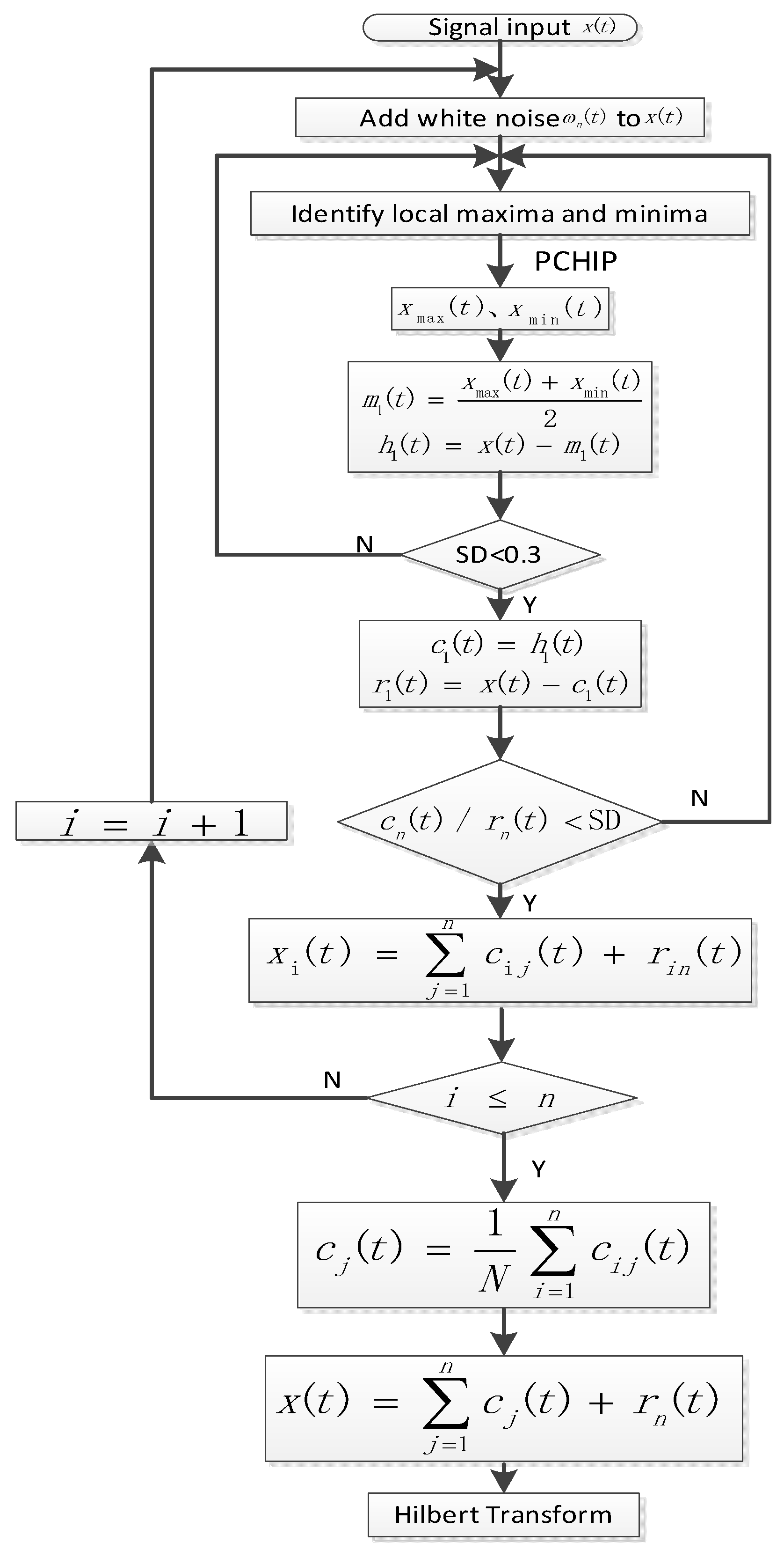
Article

Research on Power Quality Disturbance Detection Method Based on Improved Ensemble Empirical Mode Decomposition

School of Technology, Beijing Forestry University, Beijing 100083, China
*
Author to whom correspondence should be addressed.
Electronics 2020, 9(4), 585; https://doi.org/10.3390/electronics9040585
Submission received: 18 February 2020 / Revised: 22 March 2020 / Accepted: 28 March 2020 / Published: 30 March 2020
(This article belongs to the Section Circuit and Signal Processing)

Abstract

:
With the increasing proportion of various unbalanced loads in the power grid, power quality is seriously challenged. It is of great significance to effectively detect, analyze, and evaluate the power quality problems. First, this paper introduces the current situation of power quality (PQ) disturbance detection methods. It summarizes that the current PQ disturbance detection methods include Wavelet Transform (WT), Hilbert–Huang Transform (HHT), and Ensemble Empirical Mode Decomposition (EEMD). EEMD has a better detection accuracy, but its running time is longer. Therefore, to reduce the running time of the EEMD algorithm, this paper proposed two improvements: increasing the screening threshold and selecting piecewise cubic Hermite interpolation polynomial fitting. At the same time, the mathematical models of transient power quality disturbance and harmonic were established for comparative verification. The experimental results showed that the improved Ensemble Empirical Mode Decomposition (IEEMD) algorithm greatly reduced the running time of the algorithm on the premise of ensuring the detection accuracy. Hence, the improvement of this paper is of great significance for the industrial application of the EEMD algorithm.

1. Introduction

In the modern power system, power quality has become very unstable due to the large numbers of nonlinear loads and generators in the grid. Notably, power electronic-based systems such as adjustable speed drives, power supplies for IT-equipment, high-efficiency lighting, and inverters in systems generating electricity from distributed renewable energy sources are sources of disturbances [1]. The power quality (PQ) not only affects the operation of the power system, but it is closely related to the development of the national economy. High-quality power can effectively make all parts of the power system to run efficiently and smoothly, allowing the national economy to develop at high speed. On the contrary, the cost of the power industry will increase significantly and may lead to the deterioration of the stability of the power system, which will seriously affect the national economy. Hence, it is necessary to improve the PQ.
Accurate detection of power quality disturbances is a prerequisite for improving power quality problems. Since the 1980s, researchers have proposed several detection methods [2]. This paper mainly studies the Ensemble Empirical Mode Decomposition (EEMD) algorithm and proposes improvements. The EEMD algorithm adds white noise to the signal, and then decomposes it by Empirical Mode Decomposition (EMD), and uses the filtering characteristics of white noise to suppress the mode aliasing [3]. At present, several researchers have proposed the improvement of the EEMD algorithm.
In Reference [4], the Independent Component Analysis algorithm (ICA) was combined with EEMD to ensure the orthogonality and independence of the decomposed IMF to eliminate redundancy, effectively solving the noise reduction problem and accurately extracting the signal features. In Reference [5], the auxiliary positive and negative white noise was added to the original signal, which effectively eliminated the residual auxiliary noise of the reconstructed signal. Still, the amount of calculation was further increased, which was contrary to the aging of detection. In Reference [6], comparing EMD and EEMD, EMD followed the median filter and eliminated the impulse noise in the IMF, which could significantly improve the ability to distinguish the signal feature. In Reference [7], a method based on Complementary Ensemble Empirical Mode Decomposition (CEEMD) and Singular Spectrum Analysis (SSA) was proposed, which could effectively suppress strong noise and extract weak fault features, although it took a long time.
First, this paper introduces several common PQ detection methods, such as the Hilbert-Huang Transform (HHT) and EEMD algorithm. Second, it analyzes its shortcomings and proposes an improved EEMD algorithm from the algorithm running time. Third, it establishes several PQ disturbance mathematical models, obtains the detection results of the above methods through simulation experiments, analyzes and compares their advantages and disadvantages, and finally summarizes and prospects the full text.

2. Methodologies

2.1. Hilbert–Huang Transform (HHT)

HHT is a signal processing method proposed by Huang et al. in 1998 to have strong processing and decomposition capabilities for nonlinear and non-stationary signals [8]. It mainly includes the EMD [3] algorithm and Hilbert transform.

2.2. Ensemble Empirical Mode Decomposition (EEMD)

Huang and Flandrin proposed the EEMD algorithm for the mode mixing in the EMD [9,10] method and the characteristics of the white noise decomposition process [3]. The specific decomposition steps are as follows.
(1) Add a set of white noise ω ( t ) to the original signal x ( t ) to get an overall signal X ( t ) :
X ( t ) = x ( t ) + ω ( t )
(2) Use EMD to decompose the original sequence X ( t ) after adding white noise to get n decomposed natural modal components c 1 j ( t ) and a residual component r1n(t). This manuscript sets cij(t) as EMDIMF.
X ( t ) = r 1 n ( t ) + j = 1 n c 1 j ( t )
(3) Repeat the above two steps for a total of N times, the amplitude of the white noise sequence added each time is different. X i ( t ) obtained by adding white noise to the original sequence x(t) and the EMDIMF obtained by the i-th decomposition is c ij ( t ) , the resulting margin is rin(t).
X i ( t ) = r i n ( t ) + j = 1 n c i j ( t )
(4) c j ( t ) is obtained by c ij ( t ) taking the overall average, Let c j ( t ) be the IMF in this manuscript
c j ( t ) = 1 N j = 1 n c ij ( t )
(5) Reconstruct x(t) with each IMF component and the final remaining amount:
x ( t ) = j = 1 n c ij ( t ) + r n ( t )
The white noise sequence added in the above steps should obey the normal distribution of ( 0 , ( α ε ) 2 ) , where α is the intensity parameter of the noise, and ε is the standard deviation of the signal.

2.3. Improved Ensemble Empirical Mode Decomposition (IEEMD) Method

The EEMD algorithm in Section 2.2 solves the mode mixing problem of the EMD algorithm, but it also leads to a severe drawback, i.e., its operation for a long time. To improve the running speed and not affect the accuracy of power quality detection, we chose to improve the EEMD algorithm from two aspects: algorithm running time and envelope fitting effect. The specific flow chart is shown in Figure 1.

2.3.1. Algorithm Runtime Improvement

Usually, to reduce the running time of the program, we can reduce the number of loops of the algorithm. In the EEMD algorithm, when white noise is added to obtain the IMF components of each order, the problem of how to screen out the IMF is involved. The traditional EEMD method takes the standard deviation of two consecutive screening components as the measurement standard. Whether the screening process ends is judged by comparing it with the screening threshold. Therefore, this paper chose to increase the screening threshold appropriately without affecting the detection accuracy, thereby reducing the number of cycles, reducing the running time, and speeding up detection.

2.3.2. Envelope Fitting Improvement

The EEMD algorithm still has problems such as envelope fitting and endpoint effects. Therefore, to ensure that the screening threshold is increased while maintaining the detection accuracy, this paper chose to improve the envelope fitting.
The cubic spline method is used for envelope fitting. However, we found that the piecewise cubic Hermite Interpolation Polynomial (PCHIP) method fits the signal closer to the original signal. The two methods construct the envelope in the same way, but the method of selecting the slope is different. In general, when the data is smooth, the results obtained by spline are more accurate. When the data is not smooth, the PCHIP fit is better than a spline. Take the voltage swell as an example. Figure 2 shows the comparison result.

3. Disturbances Models

The literature addresses the modeling of PQ disturbances to verify the various detection methods in Section 2, and a series of efficient modeling algorithms have been proposed [11,12,13,14]. The unified setting of the disturbance start time is 0.07 s, and the end time is 0.14 s (pulse transient start time is 0.0996 and end time is 0.1004). The PQ disturbance signal generation models and their control parameters are shown in Table 1.

4. Experimentation and Results

All experiments in this manuscript are in Windows 10, equipped with 2.50 GHz, Intel (R) corei7-6500U CPU, and a 12 GB RAM. All simulation experiments were carried out with MATLAB R2018a (The MathWorks, Inc., Natick, MA, USA).

4.1. PQ Detection Based on EMD

The difference between EMD and EEMD is that the EMD does not add white noise to the original signal, but directly decomposes the original signal to obtain the IMF component. Therefore, there is a specific mode mixing phenomenon, which needs to be screened and judged to obtain a clear IMF component. Through the literature review, we found that the first IMF component c 1 ( t ) does not have a modal mixing phenomenon. Thus, only the Hilbert transform is performed on c 1 ( t ) to obtain the instantaneous frequency of the signal, and the detection results are shown in Figure 3, Figure 4, Figure 5, Figure 6, Figure 7 and Figure 8.

4.2. PQ Detection Based on EEMD

The test results based on the EEMD algorithm are shown in Figure 9, Figure 10, Figure 11, Figure 12, Figure 13 and Figure 14. Based on the suggestions of Huang et al. [3], not all IMF components were required for detection and analysis, so it was necessary to select and determine appropriate IMF components to express the physical meaning of signals. In this detection, the first six IMF components were selected for analysis, and the third IMF component was selected for the Hilbert transform to get the amplitude and frequency of the signal. For voltage swell, voltage sag, and voltage interruption, the integrated average number N was 110, and the noise standard deviation was 0.05. For the oscillatory transient, the N was 105, and the noise amplitude standard deviation was 0.06. For the impulsive transient, the N was 105, and the noise amplitude standard deviation was 0.08. For the harmonic, the N was 105, and the noise amplitude standard deviation was 0.15

4.3. PQ Detection Based on Improved EEMD

Based on the improved EEMD, PQ disturbance detection was similar to Section 4.2. The first six IMF components were selected for analysis, and the third IMF component was selected for the Hilbert transformation to obtain the signal amplitude and frequency. The detection results are shown in Figure 15, Figure 16, Figure 17, Figure 18, Figure 19 and Figure 20. For voltage swell, voltage sag, and voltage interruption, the integrated average number N was 110, and the noise standard deviation was 0.03. For the oscillatory transient, the N was 105, and the noise amplitude standard deviation was 0.20. For the impulsive transient, the N was 105, and the noise amplitude standard deviation was 0.05. For the harmonic, the N was 105, and the noise amplitude standard deviation was 0.14.

4.4. PQ Detection Based on Wavelet Transform (WT)

To analyze the advantages and disadvantages of the improved EEMD method more objectively, we chose the WT [14,15,16,17] as a comparison group. The test results are shown in Figure 21, Figure 22, Figure 23, Figure 24, Figure 25 and Figure 26. In general, the starting and ending time of PQ disturbances can be obtained by observing and analyzing the the changes in d1 in Figure 21, Figure 22, Figure 23, Figure 24, Figure 25 and Figure 26.

5. Discussion

In this paper, the detection time point and the algorithm run-time were taken as the comparison standard. The comparison of the detection results of the four methods is shown in Table 2, Table 3, Table 4, Table 5 and Table 6.

5.1. Time Point Accuracy

The detection results of the four detection methods for the disturbance start and stop time are summarized and compared with the actual results, as shown in Table 2 and Table 3.
To more intuitively explain the accuracy of the detection method, we compared the start and end time of the disturbance obtained by the four detection methods to the actual time. The relative error of the obtained results is calculated to obtain Table 4, Table 5 and Table 6.
Table 5 shows that compared to the EMD algorithm and the WT, the relative errors of the EEMD algorithm and the improved EEMD method for detecting the start and end time of the disturbance and the start and end time of the actual disturbance are generally small. It could be seen from the comparison results that the relative error of the improved EEMD algorithm and the traditional EEMD algorithm was almost equal. This result indicated that the improved EEMD algorithm ensured that the accuracy of the detection time point was consistent with the traditional EEMD algorithm.

5.2. Algorithm Running Time

This paper used MATLAB’s tic/toc method to calculate the time used for several detection methods. The running time of the four detection methods is shown in Table 6.
By comparing and analyzing the data in the table, we found that the running time difference between the improved EEMD algorithm and the WT method was about 0.3s. Still, the detection accuracy of this paper was higher than the WT method. Compared to the EEMD, the running time of the improved EEMD method was reduced significantly, and the running time was saved by nearly 6s, which was only 14.61% of the running time of the traditional EEMD. The results showed that the improved EEMD was significantly better than the traditional EEMD in terms of the algorithm running speed.

6. Conclusions

This paper mainly focuses on the problem that the EEMD algorithm is applied to power quality disturbance detections when the running time is too long. We proposed an improved method for ensuring the detection accuracy and reducing the duration of the EEMD algorithm. Concurrently, to objectively and dialectically analyze the advantages and disadvantages of the improved EEMD method, the detection results are compared with the EMD, EEMD, and WT. This proved that the improved EEMD algorithm dramatically reduced the operation time of the algorithm on the premise of ensuring the high accuracy of detection time. Of course, there are still some shortcomings in this paper, mainly because the EEMD algorithm lacks specific adaptability and needs further thinking. At the same time, the disturbance signals proposed in the example simulation of this paper are too ideal and straightforward, and there is a particular gap with the actual field data. Next, we will verify a large amount of field data and continually modify the algorithm.

Author Contributions

H.W. and J.L. conceived the overall approach and made the same contribution; S.L. has made the simulation; X.X. provided suggestions about the detection strategy. All authors have read and agreed to the published version of the manuscript.

Funding

The Central Universities supported this research under Grant BLX2014-05. The National Natural Science Foundation of China under Grant 51605031, and the China Postdoctoral Science Foundation under Grants 2018T110055 and 2016M600051.

Conflicts of Interest

The authors declare no conflict of interest.

Abbreviations

PQpower quality
WTWavelet Transform
HHTHilbert-Huang Transform
EMDEmpirical Mode Decomposition
EEMDEnsemble Empirical Mode Decomposition
IMFIntrinsic Mode Function
IEEMDImproved Ensemble Empirical Mode Decomposition
PCHIPPiecewise Cubic Hermite Interpolation Polynomial
SSASingular Spectrum Analysis
CEEMDComplementary Ensemble Empirical Mode Decomposition
ICAIndependent Component Analysis algorithm

References

  1. Driesen, J.L.; Belmans, R.J. Wavelet-based power quantification approaches. IEEE Trans. Instrum. Meas. 2003, 52, 1232–1238. [Google Scholar] [CrossRef]
  2. Khokhar, S.; Zin, A.A.B.M.; Mokhtar, A.S.B.; Pesaran, M. A comprehensive overview on signal processing and artificial intelligence techniques applications in classification of power quality disturbances. Renew. Sustain. Energy Rev. 2015, 51, 1650–1663. [Google Scholar] [CrossRef]
  3. Wu, Z.; Huang, N.E. Ensemble empirical mode decomposition: A noise-assisted data analysis method. Adv. Adapt. Data Anal. 2009, 1, 1–41. [Google Scholar] [CrossRef]
  4. Li, X.-F.; Liu, M.-J.; Wang, S.-H. Research on the EEMD algorithm of penetration acceleration signal processing based on independent component analysis. In Proceedings of the 2010 3rd International Congress on Image and Signal Processing, Yantai, China, 16–18 October 2010; Volume 9, pp. 4135–4138. [Google Scholar]
  5. Wu, Z.; Huang, N.E. A study of the characteristics of white noise using the empirical mode decomposition method. Proc. R. Soc. A: Math. Phys. Eng. Sci. 2004, 460, 1597–1611. [Google Scholar] [CrossRef]
  6. Mishra, V.K.; Bajaj, V.; Kumar, A.; Sharma, D.; Singh, G. An efficient method for analysis of EMG signals using improved empirical mode decomposition. AEU—Int. J. Electron. Commun. 2017, 72, 200–209. [Google Scholar] [CrossRef]
  7. Jiang, L.; Wang, S.; Cui, J.; Yu, M.; Wang, J. Research on Gear Signal Denoising Method Based on CEEMD and SSA. In Proceedings of the 2019 Chinese Control and Decision Conference (CCDC), Nanchang, China, 3–5 June 2019; pp. 2751–2756. [Google Scholar]
  8. Huang, N.E.; Shen, Z.; Long, S.R.; Wu, M.C.; Shih, H.H.; Zheng, Q.; Yen, N.-C.; Tung, C.C.; Liu, H.H. The empirical mode decomposition and the Hilbert spectrum for nonlinear and non-stationary time series analysis. Proc. R. Soc. A: Math. Phys. Eng. Sci. 1998, 454, 903–995. [Google Scholar] [CrossRef]
  9. Pierleoni, P.; Palma, L.; Belli, A.; Pieri, M.; Maurizi, L.; Pellegrini, M.; Marroni, A. An EMD-based algorithm for emboli detection in echo Doppler audio signals. Electronics 2019, 8, 824. [Google Scholar] [CrossRef] [Green Version]
  10. Escalona, O.J.; Lynn, W.D.; Perpiñan, G.; McFrederick, L.; McEneaney, D.J. Data-Driven ECG Denoising Techniques for Characterising Bipolar Lead Sets along the Left Arm in Wearable Long-Term Heart Rhythm Monitoring. Electronics 2017, 6, 84. [Google Scholar] [CrossRef] [Green Version]
  11. Brito, N.S.D.; Souza, B.A.; Pires, F.A.C. Daubechies wavelets in quality of electrical power. In Proceedings of the 8th International Conference on Harmonics and Quality of Power(ICHQP), Athens, Greece, 14–16 October 1998; pp. 511–515. [Google Scholar]
  12. Sahito, F.; Zhiwen, P.; Ahmed, J.; Memon, R.A. Wavelet-Integrated Deep Networks for Single Image Super-Resolution. Electronics 2019, 8, 553. [Google Scholar] [CrossRef] [Green Version]
  13. Guo, M.; Wu, Z. Noise Reduction for High-Accuracy Automatic Calibration of Resolver Signals via DWT-SVD Based Filter. Electronics 2019, 8, 516. [Google Scholar]
  14. Zhong, T.; Zhang, S.; Cai, G.; Huang, N. Power-quality disturbance recognition based on time-frequency analysis and decision tree. IET Gener. Transm. Distrib. 2018, 12, 4153–4162. [Google Scholar] [CrossRef]
  15. Lee, C.-Y.; Shen, Y.-X. Optimal Feature Selection for Power-Quality Disturbances Classification. IEEE Trans. Power Deliv. 2011, 26, 2342–2351. [Google Scholar] [CrossRef]
  16. Janik, P.; Lobos, T. Automated Classification of Power-Quality Disturbances Using SVM and RBF Networks. IEEE Trans. Power Deliv. 2006, 21, 1663–1669. [Google Scholar] [CrossRef] [Green Version]
  17. He, S.; Li, K.; Zhang, M. A Real-Time Power Quality Disturbances Classification Using Hybrid Method Based on S-Transform and Dynamics. IEEE Trans. Instrum. Meas. 2013, 62, 2465–2475. [Google Scholar] [CrossRef]
Figure 1. Improved EEMD algorithm flow chart.
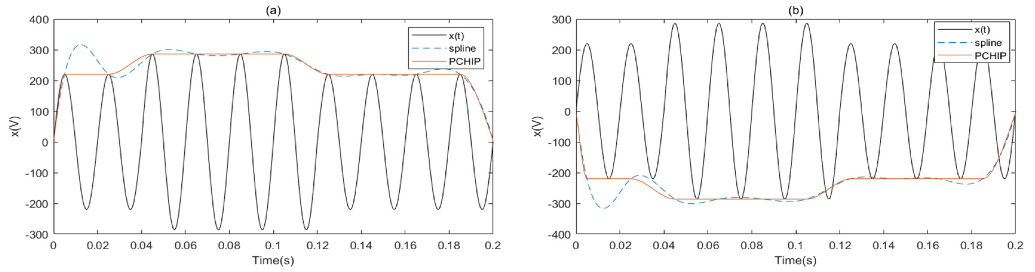
Electronics 09 00585 g001
Figure 2. Voltage swell signal upper (a) and lower (b) envelopes.
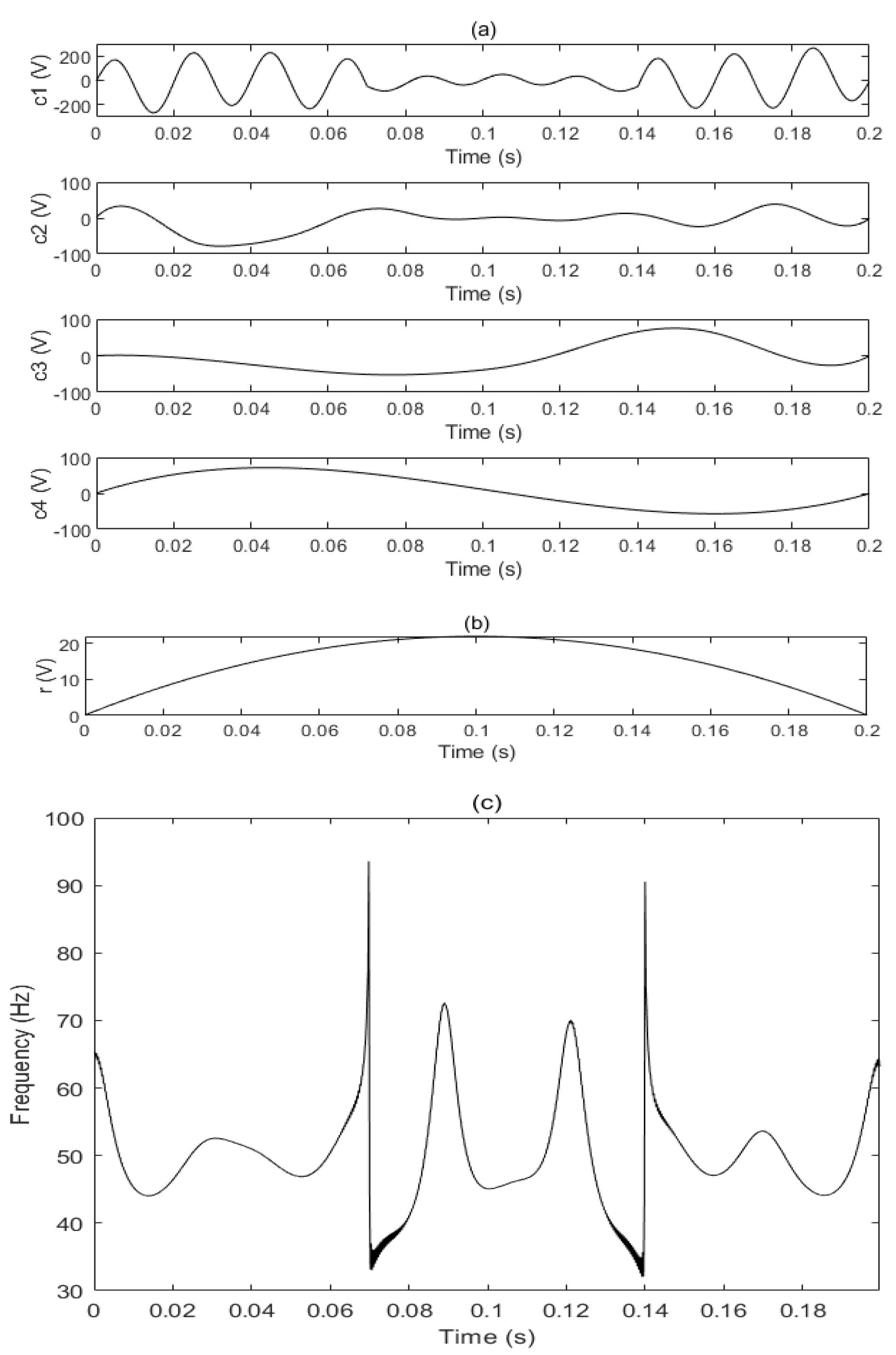
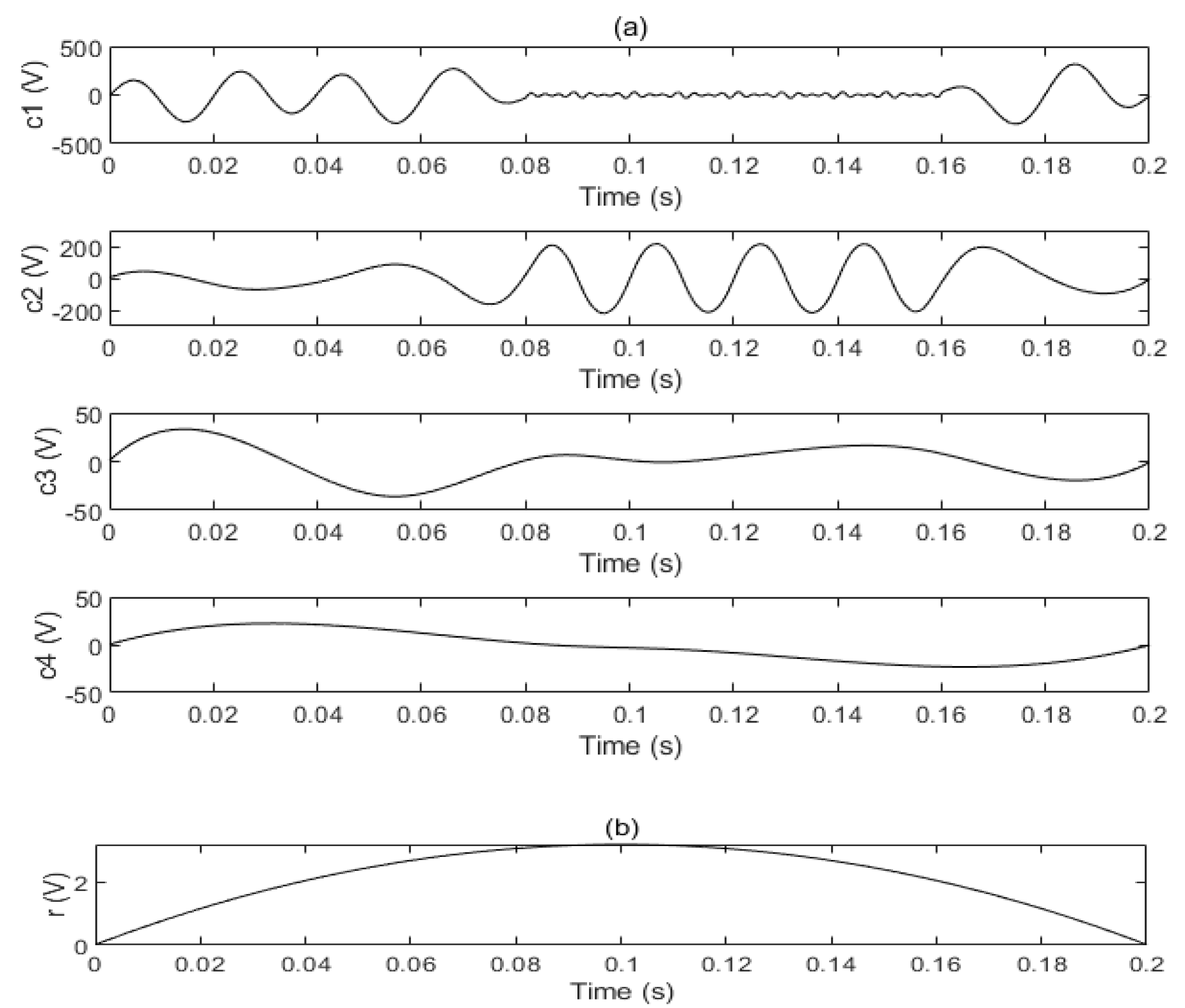
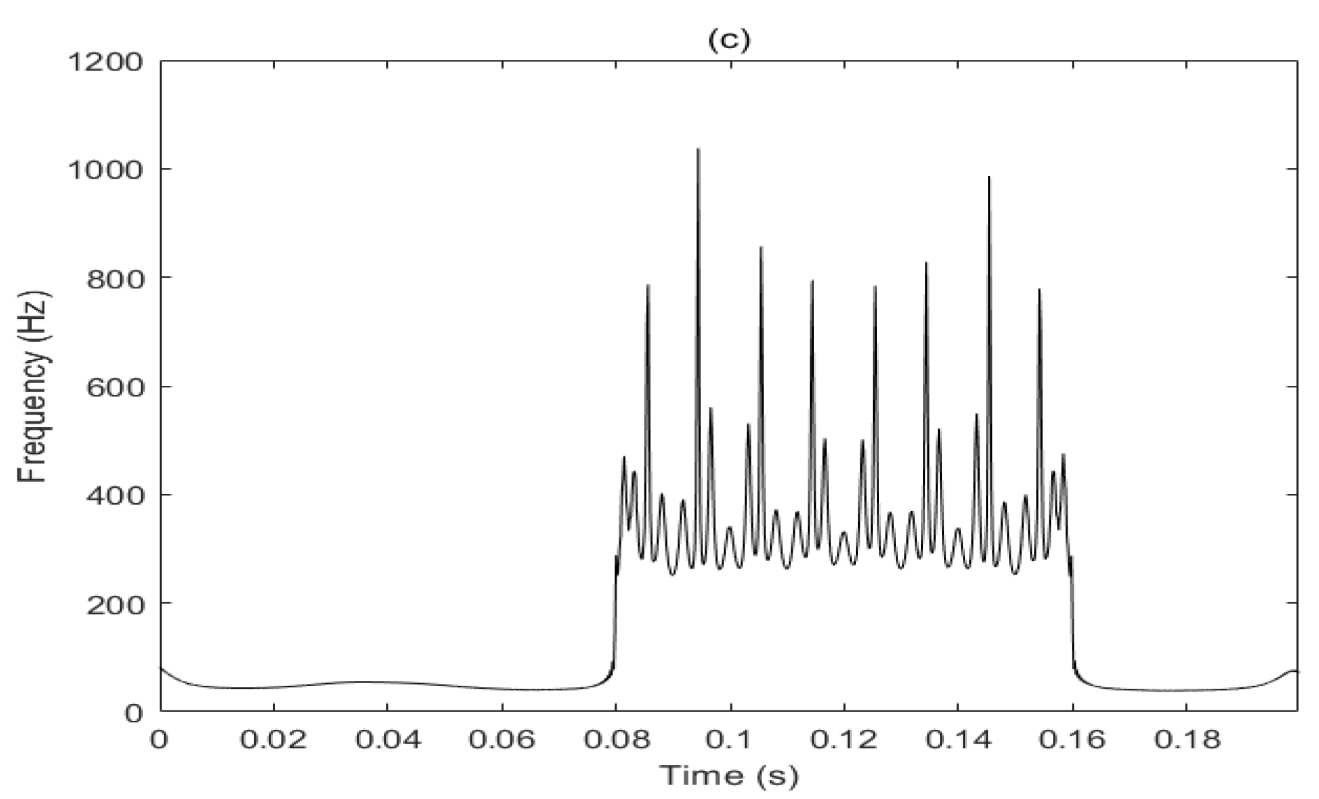
Electronics 09 00585 g002
Figure 3. Voltage swell IMF components (a), margin (b), and frequency parameter (c).
Electronics 09 00585 g003aElectronics 09 00585 g003b
Figure 4. Voltage sag IMF components (a), margin (b), and frequency parameter (c).
Electronics 09 00585 g004
Figure 5. Voltage interruption IMF components (a), margin (b), and frequency parameter (c).
Electronics 09 00585 g005aElectronics 09 00585 g005b
Figure 6. Oscillatory transient IMF components (a), margin (b), and frequency parameter (c).
Electronics 09 00585 g006
Figure 7. Impulsive transient IMF components (a), margin (b), and frequency parameter (c).
Electronics 09 00585 g007
Figure 8. Harmonic IMF components (a), margin (b), and frequency parameter (c).
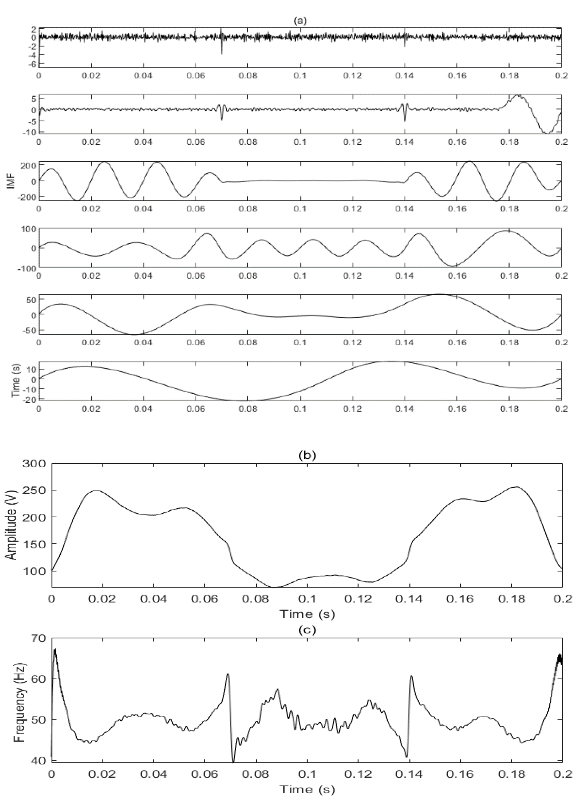
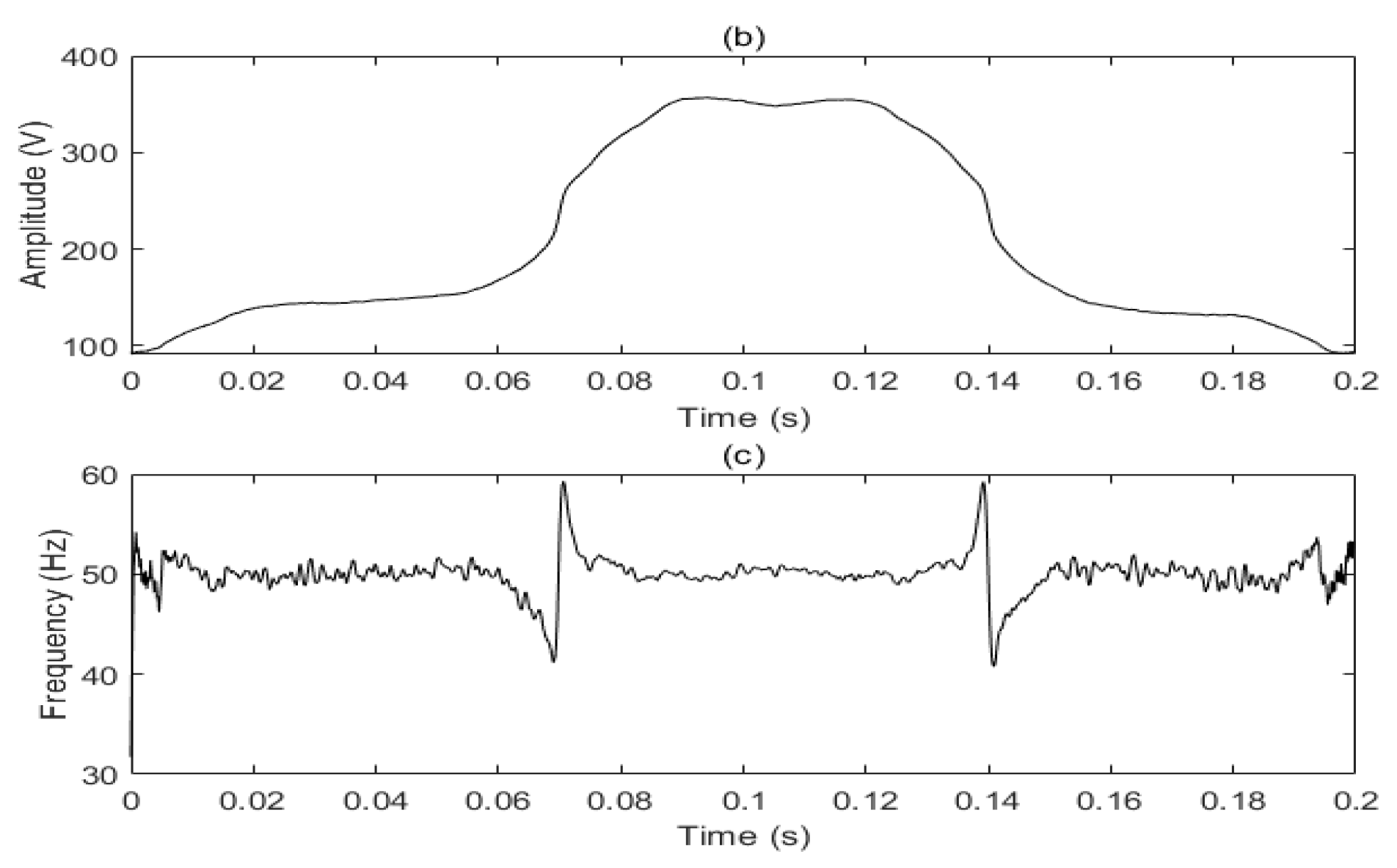
Electronics 09 00585 g008aElectronics 09 00585 g008b
Figure 9. Voltage swell IMF components (a), amplitude (b), and frequency (c).
Electronics 09 00585 g009aElectronics 09 00585 g009b
Figure 10. Voltage sag IMF components (a), amplitude (b), and frequency (c).
Electronics 09 00585 g010
Figure 11. Voltage interruption IMF components (a), amplitude (b), and frequency (c).
Electronics 09 00585 g011aElectronics 09 00585 g011b
Figure 12. Oscillatory transient IMF components (a), amplitude (b), and frequency (c).
Electronics 09 00585 g012
Figure 13. Impulsive transient IMF components (a), amplitude (b), and frequency (c).
Electronics 09 00585 g013aElectronics 09 00585 g013b
Figure 14. Harmonic IMF components (a), amplitude (b), and frequency (c).
Electronics 09 00585 g014
Figure 15. Voltage swell IMF components (a), amplitude (b), and frequency (c).
Electronics 09 00585 g015aElectronics 09 00585 g015b
Figure 16. Voltage sag IMF components (a), amplitude (b), and frequency (c).
Electronics 09 00585 g016
Figure 17. Voltage interruption IMF components (a), amplitude (b), and frequency (c).
Electronics 09 00585 g017aElectronics 09 00585 g017b
Figure 18. Oscillatory transient IMF components (a), amplitude (b), and frequency (c).
Electronics 09 00585 g018
Figure 19. Impulsive transient IMF components (a), amplitude (b), and frequency (c).
Electronics 09 00585 g019aElectronics 09 00585 g019b
Figure 20. Harmonic IMF components (a), amplitude (b), and frequency (c).
Electronics 09 00585 g020
Figure 21. Voltage swell.
Electronics 09 00585 g021
Figure 22. Voltage sag.
Electronics 09 00585 g022
Figure 23. Voltage interruption.
Electronics 09 00585 g023
Figure 24. Oscillatory transient.
Electronics 09 00585 g024
Figure 25. Impulsive transient.
Electronics 09 00585 g025
Figure 26. Harmonic.
Electronics 09 00585 g026
Table 1. Power quality disturbances models and its controlling parameters.
LabelDisturbance ClassModeling EquationsEquations’ Parameters
C0Pule Signal h ( t ) = A cos ( ω t ) A = 1 ( pu ) , f = 50 H z , ω = 2 π f
u ( t ) = { 1 , t 0 0 , t ( π 2 θ ) < 0
C1Voltage Sag h ( t ) = A { 1 k [ u ( t 1 ) u ( t 2 ) ] } cos ( ω t ) 0.1 < k < 0.9 , 0.5 T t 2 t 1 9 T
C2Voltage Swell h ( t ) = A { 1 + k [ u ( t 1 ) u ( t 2 ) ] } cos ( ω t ) 0.1 < k < 0.9 , 0.5 T t 2 t 1 9 T
C3Voltage Interruption h ( t ) = A { 1 k [ u ( t 1 ) u ( t 2 ) ] } cos ( ω t ) 0.9 < k < 1.0 , 0.5 T t 2 t 1 9 T
C4Oscillatory Transient h ( t ) = A { cos ( ω t ) + k e b ( t 2 t 1 ) cos ( c ω t ) [ u ( t 1 ) u ( t 2 ) ] } k = 0.3 , b = 0.6 , c = 7
C5Impulsive Transient h ( t ) = A { cos ( ω t ) + b [ u ( t 1 ) u ( t 2 ) ] } b = 0.6 , 0 < t 2 t 1 < 3 m s
C6Harmonic h ( t ) = A sin ( ω t ) + α 3 ( 3 ω t ) + α 5 ( 5 ω t ) + α 7 ( 7 ω t ) 0.02 < α 3 , α 5 , α 7 < 0.1
Table 2. The test results of the disturbances start time point.
Detection MethodSwellVoltage SagInterruptionOscillation TransientPulse TransientHarmonic
EMD0.06940.06960.06960.06980.09920.0698
EEMD0.06960.06990.07000.06980.09940.0698
IEEMD0.06960.06980.07000.06980.09940.0700
WT0.07020.07040.07010.06900.09780.0701
Actual time0.07000.07000.07000.07000.09960.0700
Table 3. The test results of the disturbances end time point.
Detection MethodSwellVoltage SagInterruptionOscillation TransientPulse TransientHarmonic
EMD0.13960.13940.13980.13920.10060.1398
EEMD0.13980.13960.14000.13960.10040.1401
IEEMD0.13980.13960.14000.14020.10040.1401
WT0.14010.14010.14020.14160.10200.1412
Actual time0.14000.14000.14000.14000.10040.1400
Table 4. The relative error of the disturbances start time point.
Detection MethodSwellVoltage SagInterruptionOscillation TransientPulse TransientHarmonic
EMD−0.85%−0.57%−0.57%−0.29%−0.40%−0.29%
EEMD−0.57%−0.14%0−0.29%−0.20%−0.29%
IEEMD−0.57%−0.29%0−0.29%−0.20%0
WT+0.29%+0.57%+0.14%+1.43%−1.81%+14%
Table 5. The relative error of the disturbances end time point.
Detection MethodSwellVoltage SagInterruptionOscillation TransientPulse TransientHarmonic
EMD−0.29%−0.42%−0.14%−0.57%+0.20%−0.14%
EEMD−0.14%−0.29%0−0.29%0+0.07%
IEEMD−0.14%−0.29%0+0.14%0+0.07%
WT+0.07%+0.07%+0.14%1.43%+1.59%+0.86%
Table 6. The running time of the detection methods.
Running TimeSwellVoltage SagInterruptionOscillation TransientPulse TransientHarmonic
EMD0.60510.54150.59860.58760.55800.1713
EEMD6.71086.33974.34485.42484.41224.8157
IEEMD0.98051.41371.46822.18622.15152.0306
WT0.69880.81360.67600.83850.70860.6972

