Abstract
An accurate detection and classification of scenes and objects is essential for interacting with the world, both for living beings and for artificial systems. To reproduce this ability, which is so effective in the animal world, numerous computational models have been proposed, frequently based on bioinspired, computational structures. Among these, Hierarchical Max-pooling (HMAX) is probably one of the most important models. HMAX is a recognition model, mimicking the structures and functions of the primate visual cortex. HMAX has already proven its effectiveness and versatility. Nevertheless, its computational structure presents some criticalities, whose impact on the results has never been systematically assessed. Traditional assessments based on photographs force to choose a specific context; the complexity of images makes it difficult to analyze the computational structure. Here we present a new, general and unspecific assessment of HMAX, introducing the Black Bar Image Dataset, a customizable set of images created to be a universal and flexible model of any ‘real’ image. Results: surprisingly, HMAX demonstrates a notable sensitivity also with a low contrast of luminance. Images containing a wider information pattern enhance the performances. The presence of textures improves performance, but only if the parameterization of the Gabor filter allows its correct encoding. In addition, in complex conditions, HMAX demonstrates good effectiveness in classification. Moreover, the present assessment demonstrates the benefits offered by the Black Bar Image Dataset, its modularity and scalability, for the functional investigations of any computational models.
1. Introduction
The detection and classification of scenes and objects is a key feature of the human brain, to guarantee its extraordinary effectiveness in the interaction with the external world. Reproducing the same ability of robust recognition is an essential—but still unresolved—challenge in computer vision. Numerous computational models have been proposed, each one presenting a different strategy to search and process the relevant information within images. One of the main criteria of distinction between these models consists in the fact that the model is (or not) bio-inspired. Among the bio-inspired models, the HMAX model is certainly one of the best known. This HMAX is a feedforward hierarchical feature learning model for classification tasks. Initially proposed by Riesenhuber and Poggio In 1999, and later extended by Serre and colleagues in 2005 and in 2007, its functional structure is inspired by the standard model for recognition in the primate visual stream [1,2,3,4,5,6]. Over time, numerous studies have been carried out around the computational structure of HMAX, to improve its performance or to optimize its biological mimesis [7,8,9,10,11,12,13,14,15,16,17]. Despite the time which has passed since its first presentation, HMAX still deserves great interest.
The fact that HMAX plays both the role of model of a biological system and of a technological tool used in many technical fields, makes this model unique, even compared to the new algorithms emerging in this period. Clearly, mimicking the structures and mechanisms of the primate visual cortex helps to improve our knowledge about the visual system, and promote the interdisciplinary study of computer vision and neuroscience. In this context, the functional equivalence of Gabor’s filters, and especially the selection of features are topics of current great interest. The mutual evolution between these disciplines will help to develop new solutions in computer vision, in the hope of achieving the remarkable performance that characterizes biological systems. However, there are also pragmatic reasons maintaining that the interest in HMAX is still alive; among these, the main reason is probably that its computational structure is an excellent compromise between simplicity, computational cost and performance. As well as this, in some applications, HMAX still produces results worthy of note [7,12,18].
All of these elements have led us to choose HMAX as an example of application, to present and validate a new tool: the Black Bar Image Dataset (BBID). The BBID is a new image dataset, specifically developed to perform assessments of computational models for image processing and categorization. Two characteristics make BBID a really useful tool: it allows performing universally valid assessments—unrelated to any specific context—and it also ensures the knowledge and control of each feature within each image. In the present work, we use the BBID for two fundamental assessments regarding HMAX: the evaluation of the sensitivity to specific features of images, and the measure of the influence of the ‘random patches-selection’ strategy on the results provided by HMAX. With regard to the first point, we have selected the most common features of images (to provide useful examples), modulated their magnitude, and evaluated the effectiveness of HMAX. The second point, instead, is specifically related to one of the characteristics of HMAX: the strategy that Serre and colleagues adopted to obtain the invariance to position and scale, based on the comparison of patches randomly selected, cropped from each image in different positions and scales [2]. This strategy is probably one of the most salient (and most criticized) features of the model, and was an object of analyses and revisions in subsequent research [7,14,19,20,21]. On the one hand, the random strategy allows the largest operational validity; on the other hand, it appears “not optimized” in computational and functional terms. To assess the effect of the random strategy, we defined a recursive method using the BBID in order to evaluate the variability on the HMAX outcome, probably for the first time in a quantitative manner.
The structure of the article is as follows. These next three paragraphs present, respectively: (i) a summary of the HMAX model, (ii) a summary of the classification test performed with HMAX and which originated this work (named “pre-test”), and (iii) the introduction to the BBID and the protocol of images chosen for the subsequent tests.
Subsequently, the assessment is divided into two sets of tests. In the first set, we examined the most general features regarding both the background and the main element of the image. The aim of these tests is to determine the sensitivity and the effectiveness threshold of HMAX, its reliability, and the functional criticalities. Each test condition was repeated a hundred times, in order to evaluate—at the same time—the variability induced by the random patches’ selection. In the second setoff test we compared heterogeneous features, to verify the conditions that ensure more reliable results. In the final discussion, we analyze the results with respect to the general context and features of the images. Where relevant, results are also evaluated in the light of the computational structure of HMAX.
2. HMAX: The Model
The computational structure of HMAX is inspired by the processing of visual information of the primate ventral stream. Its structure was inspired by the research on the monkey’s visual processing of David Hubel and Torsten Wiesel [5,22], who discovered that the visual information processing is composed by elaboration levels of increasing complexity, that it is composed by circuits of simple and complex cells, and that the topographical distribution of the visual field is preserved (Hubel and Wiesel received the Nobel Prize in 1981).
In the last fifteen years numerous and different models have been developed; at times following a bio-inspired approach as for HMAX, while at other times based on different computational structures and aimed at obtaining a specific performance, without any functional references to the human physiology. The abundant literature on this subject allows us to discover an ever-increasing number of models, which become more and more complex, and are sometimes obtained through the hybridization of previous models [23,24,25,26]. Nowadays, the Convolutional Neural Network (CNN) is perhaps the model getting the most attention—despite having lost its bio-inspired essence, thanks to the achievement of hitherto impossible performances. However, CNN models are extremely complex, and are featured by an extremely high computational coast. Table 1 provides a comparison of both HMAX and CNN characteristics.

Table 1.
Comparative between Hierarchical Max-pooling (HMAX) and Convolutional Neural Network (CNN) computational models.
The table summarizes the strengths and weaknesses of HMAX, and the comparison with CNN models, nowadays the object of increasing interest because of their constant growth in performance. Although the concept behind the CNN model is related to the research of Hubel and Wiesel on the primate visual system [5,22], its recent developments are oriented much more to the achievement of high performances, rather than to the constraints of the bio-justification of the model.
The present work refers to the original structure proposed by the working team of Poggio in 2007 [2]. In the original HMAX model, Riesenhuber and Poggio—and successively Serre and colleagues, tried to reproduce the structures and functions of the ventral stream, corresponding to the V1, V2, V4, PIT and AIT areas [27]. The fundamental structure of HMAX consists in an alternate succession of simple cells and complex cells layers, named S1, C1, S2 and C2. The simple cells layers (S1 and S2) aim to extract features from the input image, while the complex cells layers (C1 and C2) provide invariance to locations and scales of those features. Hereafter we summarize the functional features of each layer.
2.1. S1 Layer
This first layer consists of a Gabor filters bank, each one sensitive to a given orientation and scale. We adopted the original framework, that uses four different orientations (0°, 45°, 90°, 135°) and 16 scales (from 7 × 7 to 37 × 37 pixels), resulting in a total of 64 filters. The parameters of these filters are the same as proposed by Serre and colleagues [2]; the most important values are recalled in Table 2.
Table 2.
Parameters of Gabor filters adopted in the S1 layer.
2.2. C1 Layer
In order to provide a first level of invariance to locations and scales, each C1 unit draws from a neighborhood of S1 units, across two images of the same orientation and two successive scales, and extracts the maximum value.
2.3. S2 Layer
This third layer needs a training phase, before the use of the model, to be effective. During the training phase, several patches of different sizes are cropped from images in the C1 representation, at random positions and scales. Each patch is cropped at the same position and scale across the four orientations, and all of the values of the cropped elements are serialized in order to form a vector. Thus, cropping an s x s patch results in a vector of 4s2 components. During feed-forward, patches are cropped from the C1 outcome, at all locations and scales, and feed all S2 units of corresponding sizes.
2.4. C2 Layer
Finally, a “winner-take-all” procedure selects the best correspondence among all the S2 outcomes, therefore providing a complete invariance to the scales and locations of the features. We chose the linear transformation, instead of the Gaussian function, to guarantee an optimized response over the whole input interval. Once HMAX descriptors have been extracted, a final classifier (typically RBF, KNN or SVM) is charged to determine the corresponding category in classification. Based on results of specific tests, we adopted the KNN algorithm as our final classifier.
Literature proposes a wide body of assessment of the HMAX capability, in different specific contexts and conditions, based on image datasets of real objects and real scenes. For instance, we can found some works on the “classical” object recognition [11,17,28,29,30] (see Crouzet and Serre [31] for a review), as well as on scene classification [32,33], vehicle classification [34], face localization and identification [28,35,36], human gender classification [37] and human age estimation [38,39,40].
Each one of these studies bases its assessment on different image datasets, self-produced or coming from shared image collections (e.g., Caltech dataset [41] or the NIST Fingerprint dataset). Images could appear very similar—or sometimes very different—(in luminosity, contrast, subject, background, space distribution, etc. …), both one image to each other, and one database to another. Some sets of images are specific to a defined sector (Holidays images dataset [42], or the Caltech-UCSD Birds dataset [43]), and consequently they are highly characterized in their specific features; others sets of images are supposed to be nonspecific, but it appears impossible to measure how much they are “general”. More relevant: assessments in previous studies adopted images quite simple, or significantly complex, at a time. In any case, the complexity level of the images was not evaluated, also because—until now—there has never been defined any standard criteria.
To solve these issues, we have developed and tested the Black Bar Image Dataset, as described in the next section. Based on the paradigm “Object-of-interest on a Background”, the scalability of its structure allows us to test different computational models—not only HMAX—with specific or unspecific features, and starting with the simplest geometrical objects, to evolve in complexity up to the images of the real-world.
2.5. Final Classifier: Test and Selection
In an initial assessment we tested both KNN and SVM classifiers to compare the features and performances of both algorithms; for each one we also tested two modalities for the learning phase, with 1 and with 5 items as representative of each class (the five items corresponded to the orientations: 6°, 8°, 10°, 12° and 14° for the Class A, and 76°, 78°, 80°, 82° and 84° for the Class B; see the next paragraph for more details about bar items).
With just one item per category to learn, the SVM guaranteed good results with uniform bars (Test 1), but originated very low performances with textured bars (Test 2 and 3). We tried to obtain better results by using five items per category, but their performances did not improve [for instance: in Test 2 we obtained an average Classification Error of 31.00 ± 11.11 (mean ± s.d.) for the Class A, and of 46.70 ± 18.20 for the Class B]. However, the KNN classifier demonstrated very good performances, both with 1 and 5 items, in all the tested conditions [in the same test previously mentioned, with KNN we obtained an average Classification Error of 3.43 ± 7.77 (mean ± s.d.) for the Class A, and of 1.77 ± 4.21 for the Class B]. As consequence, we selected the KNN as final classifier, and we adopted just one item per category in the learning phase.
3. The Present Work
The origin of this present work was the result of a categorization test of different pictures performed with HMAX. This test is reported and summarized below as “pre-test”. We intentionally tested HMAX in a challenging condition. Some unexpected classifications originated by HMAX made evident a lack of knowledge about some functional characteristics of the HMAX model. In fact, although different HMAX’s features have long been highlighted and studied, little was done regarding the expected result, for instance, concerning the sensitivities of the model to those individual and specific features of the images.
Pre-Test: Real Images Do not Provide the Answer
We selected three groups of images, corresponding to the three categories “Faces”, “Bonsais”, and “Cougars”, from the CALTECH-256 image dataset [41]. Using HMAX we compared these categories two at a time, in a dichotomous classification task. Figure 1 shows the three couples of categories, and the results of tests.
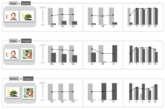
Figure 1.
Pre-Test. To assess the performances and behavior of HMAX in dichotomous classifications, we performed a battery of tests in which we compared three different categories of images: Faces, Bonsais and Cougars (from the Caltech 256 image dataset). On the left-hand, thumbnails show a sample of each category. The comparison Faces vs Bonsais was composed by 128 images per category; other comparisons were composed by 69 images per category. Histograms show the effectiveness of HMAX in each classification test: each pair of bars represents the number of items correctly classified in each category, in percentage. Different training conditions were tested. In «1a1-1a2-1a3» conditions, the HMAX was trained with only one image as representative of each class, and the same couples of images were repeatedly used in the three tests (i.e., the three trainings and tests were performed in the same conditions). In «1a-1b-1c» conditions, the HMAX was trained with one image for each category, but each test adopted a new and different couple of images. In «1-2-5-10-20» conditions, the HMAX was trained with a larger number of images (from 1 up to 20, per category), and new images were selected for each training. Class representative images were randomly selected. The black line with round markers shows the average values between categories.
Each of the histograms show, for each test, the number of items correctly classified in each category, in percentage: the light gray bars show the success rate for the left category of each pair, while the dark gray bars show the success rate for the category on the right-hand. Each pair of bars represents the results corresponding to different training/testing conditions for HMAX. Tests and results are arranged in three groups. Tests «1a1-1a2-1a3» refer to a training operated with only one image per category, and using the same images in the three tests a1, a2 and a3. Analogously, tests «1a-1b-1c» adopted only one image per category, but used a different image in each test a, b and c. In tests «1-2-5-10-20», HMAX was trained with a larger number of images, from 1 up to 20 per category; in all these tests, each new training adopted new and different images. For all tests, training images were randomly selected among the group of images of the corresponding class.
Tests with one image per category was performed to highlight the working features of HMAX in the most constraining condition, and to assess the ability of HMAX to generalize. The interest on the «1a1-1a2-1a3» testing condition is related to the random selection of patches that characterizes HMAX, which originates a different dictionary of patches at each training. As expected, results show that at each new trial, HMAX provides results different from the previous trials, even if images are exactly the same in each test, for both the training and the classification phases. This evidence suggests that a proper assessment of HMAX should consider the implications of the random selection of patches. Results of «1a-1b-1c» tests show a more accentuate variation, mainly due to the changing of the class-representative image.
Finally, the «1-2-5-10-20» tests show that a larger set of training images allows better and more stable effectiveness. Apparently, in this pre-test, HMAX provides the best results with Faces, compared to the other categories. Moreover, HMAX provides better results with the Faces category when compared to Bonsais, than when compared to Cougars. It appears interesting to discover which feature would help HMAX to classify Faces, and whether there exists a threshold to discriminate human faces from animal faces. More questions naturally arise: are the standard HMAX parameters optimized to recognize faces? Can any background characteristics help the differentiation between humans and animals? More generally, what image features influence the HMAX’s information processing? What are the thresholds of “perception” of these features? For instance, would a lighter (or darker) image produce a better result? Can we expect better results with a simplified image, for example an image defined only by contours, rather than with an image characterized by a high degree of complexity, with details and textures?
Previous works have already tried to answer some of these questions [9,17,44]. Inevitably, the use of images from the real world frequently orients or limits the analysis to a specific feature or a specific field. In some cases, these analyses were oriented to propose a modification of the computational model. Contrary to what has been done so far, we want to provide a general and universal assessment of the original and widely used structure of HMAX. For this purpose, we have defined and created the Black Bar Image Dataset (BBID), a dataset of images expressly designed to know and tune the different features within images, in a controlled and independent way.
4. The Black Bar Image Dataset (BBID)
The Black Bar Image Dataset is proposed as a model of real-world images—although extremely simplified in its first steps. The image dataset and test protocol have been created by taking inspiration from tests used in psychology and neuroscience, in order to obtain a method of analysis ready to meet the challenges of new computer vision systems. Each image is composed of a rectangular shape (the “bar”) superimposed on a selected background, to recreate the standard condition of a “defined main-element” disposed in a “defined background”. The size, color, texture and position of each component could be changed and manipulated, and are considered as variables defining and differentiating each ‘individual’.
As previously introduced, the BBID has been constructed to evaluate the performances of the HMAX, but it is also appropriate to test any other analogous computational model. The number of distinct images (hereinafter “items”) achievable through the composition of the different combinations of features is infinite. In addition, each feature can be changed solely and independently, to investigate its specific significance, or in combination with other features, to analyze any possible interaction. The button-up scalability of the image construction allows obtaining simply images, as well as images featured by a high complexity (from a simple black bar, up to a ‘real’ image: see Figure 2).
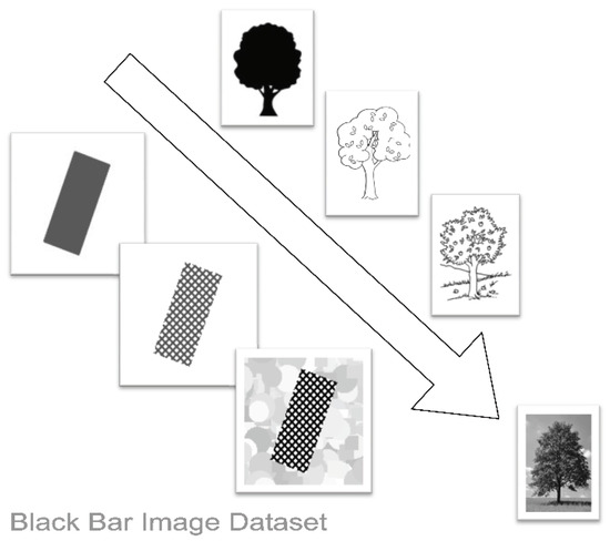
Figure 2.
Scalability of the Black Bar Image Dataset (BBID). The image resumes the BBID concept as a model of images of the real word. The arrow is oriented in the direction of the increase of: the number of elements, presence of information, the complexity, and presence of noise. This direction also involves an increase in difficulty to estimate and control features in images of the real word, whereas for a synthetic image dataset—like BBID—all parameters are controllable; an interesting and powerful feature of BBID is the possibility to evolve images up to converge to real images.
Images were 140 × 140 pixels in size, featured by a gray scale color-map (values between 001 “black” and 256 “white”). Each image contains a rectangular shape (the “bar”) as a ‘main element’, 100 pixels in length, positioned in the center. Each image was featured by different sizes and orientations of the bar: six sizes were possible for the bar width (4, 6, 9, 15, 24 or 42 pixels) and ten orientations (0°, 10°, 20°, 30°, 40°, 50°, 60°, 70°, 80° or 90° with respect to the vertical direction). A “battery” of images is composed of a collection of 60 items covering all the sizes and orientations, featured by the same texture and color for the bar, and the same texture and color for the background. Panel b of Figure 3 shows an example of the battery of images tested in the first experimental condition (uniformly-filled black bar, on a white background). In each test, HMAX must classify all the items of a battery in two classes. Two items are defined as class-representative (highlited in Figure 3 Panel B), and presented during the training phase. During the classification phase, HMAX compares each item to the class-representative items, to classify it in one of two classes on the basis of geometrical and luminance similitude criteria.
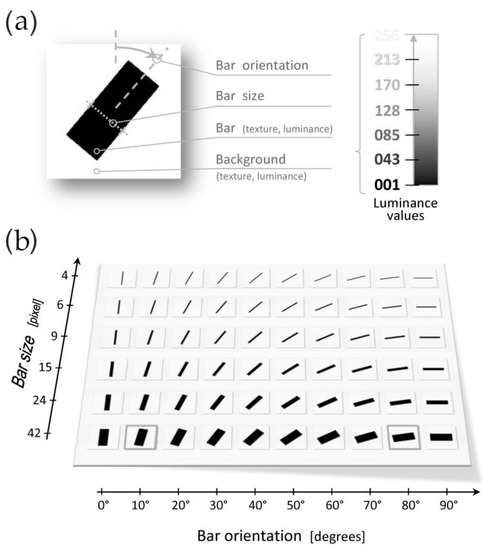
Figure 3.
Features of the BBID. Panel A: (a) A typical BBID image; the panel also presents the six parameters characterizing each item: a rectangular shape (i.e., the Bar, featured by a specific orientation and size) superposed on a selected Background, both featured by specific Luminance and Texture. For each combination of features (luminance and texture), a battery of 60 items is created by modulating the size and orientation of each Bar (6 sizes: between 4 and 42 pixels; 10 orientations: between 0° and 90°). Panel B: (b)The battery of items for the first test (uniformly filled bars, black color, on uniform white background). The two class-representative items are contoured in gray (10° and 80°).
In the Black Bar Image Dataset here presented, items are characterized by four parameters: Orientation, Size, Luminance and Texture (Figure 3 Panel A). Orientation is here adopted to differentiate and classify individual items. Size, Texture and Luminance are utilized to modulate and differentiate the available information. From the point of view of information processing, these three parameters can be associated with the notions of the “quantity”, “quality” and “intensity” of the information relevant for classification. In the tests described below, Size refers to the bar width, and varied between 4 and 42 pixels; whereas Luminance, henceforth indicated by the notation “#Lum”, varied between 001 #Lum (black) and 256 #Lum (white).
5. First Set of Tests: HMAX Sensitivity and Individual Feature Assessment
As already stated, the aim of the present research is a general and unspecific assessment of the HMAX performances in dichotomy classification tasks. This first set of tests is designed to investigate the sensitivity of HMAX to the fundamental features of the images, and their relationship to the HMAX functional structure. Special attention was paid to two functional modules, which appear to be two key-processes to guarantee the effectiveness in the classification task: (i) the convolution operated by the Gabor filters in S1 layer, and (ii) the selection and comparison of patches in S2-C2 layers.
Concerning, more specifically, the randomly operated selection of patches, this procedure could present some drawbacks, as previously stated, as well as already noticed in previous works [11,17,31]. In order to take account of this characteristic of HMAX, which can originate different results at each running, in this first set of tests each condition was repeatedly performed in 100 iterations (where an iteration was composed of a new training phase, followed by the classification phase). The purpose of the multiple iteration is to “mediate” the aleatory variability due to the random selection of patches, to provide results which are indicative of the average tendency of HMAX, in each different condition. Considering this computational peculiarity, to guarantee the easy reading of the results, the HMAX performances will be evaluated through the error rate—and not through the success rate as in the Pre-test and the second Set of tests. This first set is composed of three groups of tests. In the first group of tests (Test 1) we assessed of HMAX performances when working on uniformly filled elements. In the second group of tests (Test 2) different textures were tested to evaluate the effect on the classification performances. In the third group (Test 3) we assessed HMAX performances with images composed by textured bars on a textured background.
In all the performed tests, we selected one element per class as class-representatives for the training phase. In view of the functional characteristics of HMAX, we defined Class A by the image of the bar oriented at 10° (with respect to the vertical reference), and Class B by the image of the bar oriented at 80°, both 42 pixels in width (these two elements are highlighted in Panel b of Figure 3). These two orientations (10° and 80°) have been chosen to guarantee symmetrical and equivalent conditions for the two classes, and to avoid confusion between classes. All trainings were performed with black filling or black texture bars. To investigate the effect of the reduction of the available information, in each battery we modulated the bar width-Size between 42 and 4 pixels (respectively corresponding to 30% and 3% of the image width); this Size interval has been chosen also to cover the entire range of Gabor Filter patches widths. Based on the similitude criteria featuring HMAX, we expect that all items oriented between 0° and 40° (the left part of the battery of images) will be classed in the Class A, and all the items oriented between 50° and 90° (the right part of the battery) will be classed in the Class B. The reduction of the “items reading” capability, or of the categorization capabilities, will bring HMAX to produce a greater number of errors in the border area between Class A and Class B. Figure 3 shows an example of a battery of images, corresponding to the first experimental condition (black uniformly-filled bar). To evaluate HMAX’s performances in the case of reduction of the intensity of information pertinent for classification, we also modulated the Luminance of bars, in all three Tests.
The classification of bars is based on geometrical criteria, and needs a certain amount of information to be carried out effectively. In this sense, we will use the term “information” to indicate the specific data present in the images, relevant for the task accomplishment.
To measure the performances of HMAX, we define the Classification Error (CE), which is the sum of errors in classification for each individual item, and which occurred in over 100 identical and consecutive trials (each one composed of the initial training phase, and the successive working/classification phase).
Consequently, CE is a measure of the loss-of-effectiveness in classification, expressed in percentage. The larger is the CE, and the poorer and unreliable are the performances. Quantitatively speaking, CE values near to zero refer to a precise and accurate classification. The more the CE values get close to 50, and the more the probability of a correct classification gets close to the chance. Any CE value greater than 50 reveals a process that produces wrong results more frequently than the right ones.
5.1. Test 1 – Uniformly Filled Bars
The aim of the first group of tests is the assessment of the HMAX performances in the classification of uniformly filled elements. The adoption of a uniform background in the present tests provides evidently a model of images featured by uniform backgrounds, as well a model of images featured by a background non-uniform, and unchanged in all items.
In the first part of this assessment we manipulated the Luminance of Bars, to investigate the effect of the different intensities of the information pertinent for the classification. In the second part we assessed HMAX performances with different Background Luminance values, to verify the effect of the Luminance contrast between bar and background. Our expectation is that the more pronounced is the information compared to the background (i.e., the contrast of Luminance between bar and background), then the more effective would be the HMAX in the classification task.
In the first six tests we evaluated six different Luminance values for bars, evenly spaced between black and white (white excluded): 001, 043, 085, 128, 170 and 213 #Lum; backgrounds were white (256 #Lum) in all conditions. At the same manner, in the subsequent six tests we evaluated six different Luminance values for background, evenly spaced between black and white (black excluded): 043, 085, 128, 170, 213 and 256 #Lum; bars were black (001 #Lum) in all conditions.
5.2. Results
Figure 4 resumes the outcomes of the six tests on different Bar Luminance. Panel a shows the mean CE values, one point for each Luminance condition. In Panel b each graph shows the detailed results for each individual test; in each histogram X and Y axes present, respectively, the ten orientations and the six sizes characterizing each item, as previously presented in Panel b of Figure 3. As already illustrated, a condition characterized by larger CE values indicates a loss of effectiveness (and a loss of reliability).
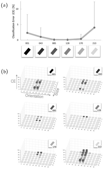
Figure 4.
Uniform Bars on uniform Background: manipulation of Bar Luminance. To measure the HMAX performances we define the Classification Error (CE), which is the sum of classification errors, which has occurred over 100 trials, for each individual item. Consequently, CE is a measure of the loss-of-effectiveness in classification, expressed in terms of percentage: the larger is the CE, and the poorer and unreliable are the performances. (a) Results of tests on uniformly filled Bars on a white background; the graph presents the mean values and standard deviations of CE for the six experimental conditions, corresponding to six Luminance values reported in the X-axis. The graph reveals that HMAX provides the best results with mid-range Luminance Bars. (b) Detailed results for each Luminance condition (luminance value is specified under the Bar icon). In each histogram, X and Y axes report, respectively, the ten orientations and the six sizes characterizing each item, as previously presented in Figure 3.
The analysis of results reveals some interesting elements. HMAX demonstrates a generalized high effectiveness in classification. The CE mean value all over the six tests is equal to 1.33 ± 3.24 (mean value ± standard deviation); the larger error in Panel a (corresponding to the lightest bar condition) is equal to 4.02 ± 8.29 (mean CE ± s.d.).
The second interesting result is clearly represented by the curve of the graph. Contrarily to the expectations, the error is not decreasing with the Luminance contrast increasing; instead, we can note an improvement of performances for bars filled with middle-tone grays (085 ~ 128 #Lum), where the error drops to zero. More detailed results could be found in Panel b, in which the errors clearly appear ascribed only to the 40° and 50° oriented bars, corresponding to the “border area” between Class A and Class B (in the following we will refer to this area as “class border area”).
Figure 5 shows the results of the six tests concerning the manipulation of Background Luminance. In this case, differently from the previous condition, these six tests produce very similar CEs both in value and in distribution over each battery. The error still remains concentrated in the class border area. Moreover, we can note that a discontinuity in the CE values, between small and large sizes, is present in all the six conditions; the same discontinuity, less pronounced, could be found also in Panel b of Figure 4. More detailed results are reported in Table 3 and Table 4.
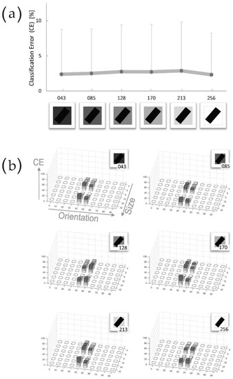
Figure 5.
Uniform Bars on uniform Background: manipulation of the Background Luminance. (a) Results of tests on black Bars on uniformly filled background; the graph presents the mean values and standard deviations of CE for the six experimental conditions, corresponding to six Luminance values reported in the X-axis. (b) Detailed results for each Luminance condition (specified in each superposed image). In each histogram, X and Y axes report respectively the ten orientations and the six sizes characterizing each item, as previously presented in Figure 3.
Table 3.
Results of the first group of tests: uniform Bar on uniform Background, Bar Luminance manipulation.
Table 4.
Results of the first group of tests: uniform Bar on uniform Background, Background Luminance manipulation.
5.3. Test 2 – Textured Bars on Uniform Background
This second group of tests investigates the HMAX performance when working with images containing textured elements.
A large body of research already tested Gabor filter and HMAX as texture classifier [45,46,47,48]. Differently from these previous works, the aim of our second group of tests is a classification based on geometric criteria, in which textures represent a contextual information common to all items.
We investigated if the presence of textures implies a facilitation for the classification task, by providing a larger amount of data, and increasing the difference between bar and background; or if the presence of textures, then to make the task more difficult, because of the addition of noise to the information concerning shapes.
Each image was composed by a textured bar on white background. Six Types of texture were tested to investigate if the spatial organization of the texture influences the task. We also manipulated the Luminance of the textures, to verify if the previous results could be extended to textured elements.
The six texture Types were characterized by two different geometric patterns (hereafter indicated as “Granularity”: “S” small, and “L” large) and three different spatial Densities (40%, 60% and 80%). Figure 6 shows the six textures and provides an enlargement of each one. We preferred nondirectional textures to prevent anisotropic interactions with the Gabor filters. Each texture was tested in four different Luminance conditions, evenly spaced between black and white (white excluded): 001, 064, 128 and 192 #Lum. The textures orientation was constant and unrelated to the orientation of the bar.
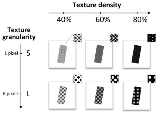
Figure 6.
Textures. Six different Textures are tested in the second group of tests, resulting from the combination of three possible densities (40%, 60% and 80%) and two possible granularities (1 or 8 pixels in diameter, respectively Small “S” and Large “L”). Each texture was tested in four different Luminance values: 001, 064, 128 and 192 #Lum.
Results
Figure 7 and Figure 8 resume the outcomes of this second group of tests, respectively, for Small and Large granularity. As shown in the Panel a of Figure 7, HMAX guarantees good performances when working with Small textures: in all conditions the error remains below the 3%, and the CE mean value over the group of twelve tests is equal to 0.87 ± 2.20 (mean value ± standard deviation). Detailed results are reported in Table 5 and Table 6. In Panel a, the three solid lines represent 40%, 60% and 80% texture Density (respectively from light-gray to black). The more detailed results, presented in Panel B, reveals that the CE error—when present—still remains limited to the class border area. Interestingly, also in Small texture conditions, performances improve, and the errors drop to zero when the Luminance attains its average value (128 #Lum).
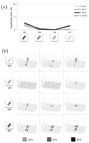
Figure 7.
Textured Bars on uniform Background: Small granularity texture. Results of the second group of tests, in which HMAX was assessed when working on textured elements on uniform background. Results here presented refer to the Small granularity texture (1 pixel in diameter). (a) Mean values for the twelve experimental conditions (4 Luminance × 3 Density conditions). The three texture densities are represented by three solid lines (80%, 60% and 40%); the dotted line reports the result from previous tests (uniform filling is equal to 100% density; some values are obtained by interpolation). The four Luminance conditions are reported on the x-axis (respectively 001, 064, 128 and 192 #Lum). Results show that also in this case, HMAX provides best results with mid-range Luminance Bars. (b) Detailed results for the twelve different Texture conditions (4 Luminance—in row, and 3 densities—in column). In each histogram, X and Y axes report respectively the ten orientations and the six sizes characterizing each item, as previously presented in Figure 3.
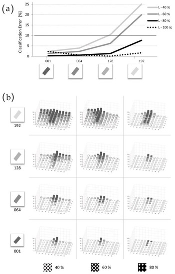
Figure 8.
Textured Bars on uniform Background: Large granularity texture. Results of the second group of tests, in which HMAX was assessed when working on textured elements on uniform background. Results here presented refer to the Large granularity texture (8 pixels in diameter). (a) Mean values for the twelve experimental conditions (4 Luminance × 3 Density conditions). The three texture densities are represented by three solid lines (80%, 60% and 40%); the dotted line reports the result from previous tests (uniform filling is equal to 100% density; some values are obtained by interpolation). The four Luminance conditions are reported on the x-axis (respectively 001, 064, 128 and 192 #Lum). (b) Detailed results for the twelve different Texture conditions (4 Luminance—in row, and 3 densities—in column). In each histogram, X and Y axes report, respectively, the ten orientations and the six sizes characterizing each item, as previously presented in Figure 3. Diagrams show that HMAX is less performing with large texture, and performances become even worse if less information is available (i.e., when bars become smaller, or lighter).
Table 5.
Results of the second group of tests: textured Bar on uniform Background, Bar “Small” Texture manipulation (Luminance and Density).
Table 6.
Results of the second group of tests: textured Bar on uniform Background, Bar “Large” Texture manipulation (Luminance and Density).
Conversely, the Large granularity texture originated larger errors, mainly at the smaller bar Size, where the larger texture causes a loss of definition of bars. In Figure 8, Panel a shows the results for the three different texture Densities (40%, 60% and 80%), and permits the comparison with the uniform-black filling condition (i.e., the 100%; dotted line in the graph). As evident, performances are very good for black bars, and deteriorate with the bar Luminance increase. The analysis of the outcome of each individual test (Panel b) reveals that errors are now present, not only in the class border area, but also in correspondence of the smaller widths bars. The average error over the twelve tests is equal to 6.78 ± 6.36 (mean ± s.d.); the most critical condition originates a CE value equal to 49.50 (corresponding to the conjunction between the class border area and the smallest bar sizes, in 40% density and 192 #Lum condition).
5.4. Test 3 – A Model of Real Word Images: Textured Bars on a Textured Background
The third group of tests investigated HMAX performances when working with textured bars on a textured background. Bars were featured by a medium granularity texture, 4 pixels in size, 60% density. Bar texture was black (001 #Lum) in all tests. About the Background: we realized a specific texture composed by a random distribution of squares and circles, to guarantee the presence of both straight and curved lines. During the tests we manipulated the Size and Luminance of squares and circles, to investigate the effect on the classification task. The size of these background elements varied from 4 × 4 to 22 × 22 pixels; the whole interval was divided into three consecutive conditions: between 4 and 10 pixels, between 10 and 16 pixels and between 16 and 22 pixels. At the same manner, the whole Luminance range was divided into four intervals evenly spaced: between 001 and 063 #Lum, between 064 and 127 #Lum, between 128 and 191 #Lum and between 192 and 256 #Lum. The texture weft was randomly generated, and was different for each item.
Results
Figure 9 presents the results of the last group of tests, in which we manipulated the background texture both in Luminance and in Granularity. One of the more evident outcomes is the presence of large errors in the darker condition (i.e., background texture Luminance < 064 #Lum), independently of the texture granularity. In all the other conditions, HMAX shows very good performances, practically unaffected by the luminance or the granularity of the background. The mean CE value over each battery of image is similar in the twelve conditions (between 3% and 6%). More detailed results are reported in Table 7.
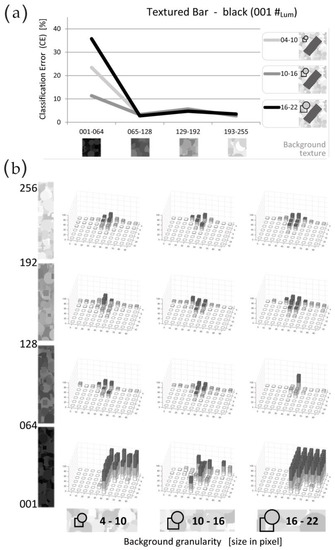
Figure 9.
Textured Black Bars on textured Background—black bar. In the third group of tests, we assessed HMAX when working on images composed by textured bar on textured background. The background texture was composed by a random distribution of squares and circles; 12 experimental conditions are originated by three possible texture sizes (i.e., Granularity) and four possible texture Luminance values. The adopted bar texture was the “Large” black texture, 60% density, already used in previous tests. (a) CE mean value resulting from each test; the three different lines refer each one to a different background Granularity (04–10, 10–16, or 16–22 pixels in diameter). Our X-axis presents the four consecutive intervals of background Luminance. (b) Detailed results for each one of the 12 Texture conditions (4 luminance values—in row, and 3 granularities—in column). In each histogram, the X and Y axes report respectively the 10 orientations and the 6 sizes characterizing each item, as previously presented in Figure 3. Diagrams show that HMAX guarantees accurate and precise results in all conditions but in the darkest, where results diverge due to the low luminance contrast between bar and background.
Table 7.
Results of the third group of tests: textured Bar on textured Background—Background Texture manipulation (Granularity and Luminance).
Figure 10 presents, for each condition, the three parameters of performance evaluation: Precision, Recall and Score.
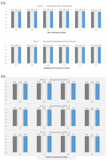
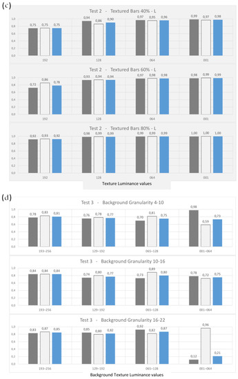
Figure 10.
Classification performance analysis. In order to measure the classification capability of HMAX, we estimated three performances parameters according to each individual condition of the three different group of tests carried out. In order to apply the calculation, we assumed the Class A as the positive factor to be identified. For each condition, Precision (dark gray bars), Recall (light gray bars) and Score (blue bars) are calculated; the corresponding numerical values are shown above each bar. (a) The horizontal axis shows the six values corresponding to the luminance values tested for the Bar (upper graph), and for the Background (lower graph). The values indicate that with uniform Bars on a uniform Background, performance is high, and the three coefficients are close to unity. (b,c) present the results, respectively, for the Small and Large textures that characterize the Bars in the second group of tests. The horizontal axis indicates the luminance values adopted for the different Bar textures. The graphs allow us to identify the condition of slight weakness that appears with the larger textures and lighter color, i.e., the condition in which the bar definition tends to reduce to zero within the white background. (d) The three lines of diagrams refer to the three granularity intervals tested for the background in this third group of tests—the granularity values are indicated in the respective titles. Each horizontal axis shows the different luminance values attributed to the background texture. We can observe a small reduction in performance, compared to the conditions of previous tests. We can see that the condition corresponding to the darker texture appears the most critical, and that when combined with a larger background granularity, the system’s discrimination capabilities fall to very low values (corresponding to the last histogram: background granularity = 16–22, background luminance 001–064; in this condition the system diverges, classifying the almost totality of items in only one category—the Class B in this case, as evident in Figure 9—and therefore generating a high number of false positives and of true negatives).
The simple structure of the BBID makes it possible to easily follow and interpret the information processing carried out by HMAX. Figure 11 provides some examples of the convolution of some previously-tested conditions. The figure shows the post-convolution images in their entirety; the patches used for comparison and classification are sub-areas selected from these images. For instance, a patch constituting the “dictionary” for classification, and enclosing an angle of bar, will allow a correct identification of the same element only if the pooling and the convolution have correctly preserved and encoded the information necessary for classification. Panel A of Figure 11 shows the presence of overshootings at the edges of the bar, compared to panel B. Panel C shows that the “S” texture granularity of bars is not correctly encoded, and the result is largely similar to that of panel B. The last four panels show that the background texture introduces a large noise, which in the cases corresponding to Panel i and g make difficult or impossible the identification of the bar, and the information needed for a correct classification is lost.
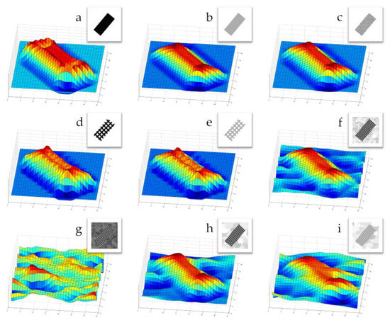
Figure 11.
Examples of BBID images convolution. Each panel shows the original BBID image and its convolution; they correspond, respectively, to: (a) black-filled bar on white background; (b) gray-filled bar (170 #Lum) on white background; (c) black textured bar (001 #Lum, 40% “S” texture) on white background; (d) black textured bar (001 #Lum, 60% “L” texture) on white background; (e) gray textured bar (170 #Lum, 60% “L” texture) on white background; (f) black textured bar (001 #Lum, 60% “M” texture) on textured background (04-10 granularity, 192–255 luminance); (g) black textured bar (001 #Lum, 60% “M” texture) on darker textured background (04–10 granularity, 065–128 luminance); (h) black textured bar (001 #Lum, 60% “M” texture) on larger-textured background (16–22 granularity, 192–255 luminance); (i) gray textured bar (128 #Lum, 60% “M” texture) on larger-textured background (16–22 granularity, 192–255 luminance).
6. Second Set of Tests: Comparison of Features
In this section, we further explore results and indications obtained in the previous tests. The first set of tests was intended to revise the main functional characteristics of HMAX, and the sensibility toward the fundamental features within images; in this second set of tests, instead, we compare the most common features to identify which conditions guarantee the best performance for HMAX. In this respect, results of previous tests already provided important suggestions. Here we focus on some emblematic cases, adopting the same analytical paradigm previously employed in the pre-test: HMAX is called to classify a group of images, belonging to two distinct BBID’s categories (each one of the two battery of images is composed of 60 images, i.e., 10 orientations × 6 sizes). The two batteries differ on the basis of a single specific feature. The differentiation feature could be the luminance of the bar, the type of filling, a different granularity of the texture, or something else. The population to classify consisted in a mixed group of 120 items. Please refer to the “Pre-Test” paragraph for more details. The only difference from the pre-test lies on the training for the ‘1a1, 1a2, 1a3’ tests, for which in the present case the items are not randomly selected, but they always correspond to the 40° orientated bar, 42 pixels wide, for each respective category.
The analyses performed in the previous set of tests showed that the presence of textures provides a larger quantity of useful information, but only if the Gabor filter is able to “read” and process the texture’s pattern. On the basis of this previous result we can expect that the presence of “good” textures would improve the capability of HMAX to correctly recognize and class the images and their elements. Figure 12 and Figure 13 show the results of six dichotomous classification tests. The first two panels present the comparison between ‘uniformly filled’ and ‘textured bars’, in dark gray and successively in light gray color. Subsequent panels present the comparison between a “generic” conditions (textured bar on a textured background, on the left-hand in each pair of images), and similar images featured by (i) a lighter bar texture; (ii) the absence of the background; (iii) a lighter background; and finally (iv) a larger granularity background.
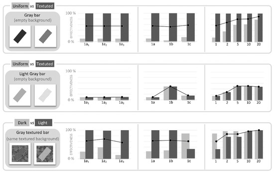
Figure 12.
Second set of tests: comparison of performances with different image categories. To assess performances of HMAX in classification, in a second set of tests we compared in pairs different categories of BBID images, analogously to what was done in the pre-test. Thumbnails on the left-hand show a sample each category. Each category was composed by a complete battery of 60 images (10 orientations, and 6 sizes). Histograms show the effectiveness of HMAX in each classification test: each pair of bars represents the number of items correctly classified in each category, in percentage. Different training conditions were tested. In «1a1-1a2-1a3» conditions, the HMAX was trained with only one image as representative of each class, and the same couples of images were repeatedly used in the three tests (i.e., the three tests were performed in the same conditions). In «1a-1b-1c» conditions, the HMAX was trained with one image for each category, but each test adopted a new and different couple of images. In «1-2-5-10-20» conditions, the HMAX was trained with a larger number of images (from 1 up to 20, per category), and new images were selected for each training. Class representative images were randomly selected. Black line with round markers shows the average values between categories.
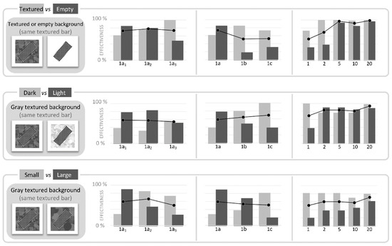
Figure 13.
Second set of tests: comparison of performances with different image categories. To assess performances of HMAX in classification, in a second set of tests we compared in pairs different categories of BBID images, analogously to what was done in the pre-test. Thumbnails on the left-hand show a sample each category. Each category was composed by a complete battery of 60 images (10 orientations, and 6 sizes). Histograms show the effectiveness of HMAX in each classification test: each pair of bars represents the number of items correctly classified in each category, in percentage. Different training conditions were tested. In «1a1-1a2-1a3» conditions, the HMAX was trained with only one image as representative of each class, and the same couples of images were repeatedly used in the three tests (i.e., the three tests were performed in the same conditions). In «1a-1b-1c» conditions, the HMAX was trained with one image for each category, but each test adopted a new and different couple of images. In «1-2-5-10-20» conditions, the HMAX was trained with a larger number of images (from 1 up to 20, per category), and new images were selected for each training. Class representative images were randomly selected. Black line with round markers shows the average values between categories.
7. General Discussion
In the present research we have evaluated the HMAX capabilities in a dichotomous classification task. To this aim, we have conceived and used the Black Bar Image Dataset (BBID), a flexible tool useful to assess performances in identification and classification tasks, and to analyze the information processing for computational models like HMAX.
In the first set of tests, three groups of tests were conducted, each one centered on specific image features: (1) uniformly filled bar on uniform background; (2) textured bar on uniform background; (3) textured bar on textured background. We defined the Classification Error (CE) as the number of incorrect classifications over 100 trials. Consequently, the CE measures the loss of effectiveness and reliability in classification, expressed in percentage.
7.1. Uniformly Filled Bars
With uniformly filled bars on uniform background, HMAX demonstrated a remarkable performance despite the edges dividing—and defining—geometry and background, were the only information available (as consequence of the initial convolution).
The good effectiveness in classification demonstrates that the patches-matching process, in the C2 layer, remains effective also when constrained to measure the similitude on the basis of a low amount of information. A subsequent analysis of the working features shows the relevance of some functional interactions between patches’ selection and image features. For instance, larger patches can embrace larger portions of the principal element within the image, thus being able to encode its width, and use this information to measure the resemblance between images. Similarly, patches that do not encounter edges cannot encode orientation-related information, while patches crossing the edges encode edge direction, as well as positional information such as the relative position between elements (left/right, up/down, or near/far).
Surprisingly, good performances were obtained also with the lightest bar (213 #lum) on white background, and black bar (001 #lum) on the darker background (043 #lum). We can state that, in the absence of noise, HMAX shows good sensitivity also at low luminance contrast. In all tests the error was concentrated in the border area between classes (corresponding to the 40° and 50° orientation bars). Moreover, no errors are found for bar orientations of 0° and 90°, although these two categories appear equivalent on the basis of the simple edges orientation information. The effectiveness of HMAX in these conditions reveals the useful contribution of the larger scales of patches, in S2-C2 layers, which are able to encode a larger part of the geometry, to differentiate 0° and 90°. To verify this point, we carried out a specific test with smaller patches (limited to 10 pixels per side); the test originated significantly larger CE values for both 0° and 90° orientations, and confirmed the important role of the largest patches. The same test showed a second factor that improves HMAX performances in this case: statistically speaking, smaller patches fall more frequently outside the bars, or completely within the contour of the bar, therefore losing effectiveness. This condition leads to reconsider the presence of pertinent information, not only in term of ‘quantity’, but also in term of the ‘probability of exploitation’.
Concerning the manipulation of the Bar Luminance, the better results obtained by the middle Luminance Bar conditions—remarkable both in terms of accuracy and precision—appears to be justified by a better performance of the final classifier in this condition. A deeper analysis, possible through the modularity of the elements of BBID, revealed that two distinct factors—originated in the first layer—influenced the final classifier: (i) Concerning the lower Luminance bars (e.g., 001 #lum black bar), its borders originate a more irruent response of the Gabor filter: due to the high luminance contrast, its convoluted image presents three or four “waves” at each bar side (depending on the filter direction), the higher in magnitude compared to other luminances. (ii) Concerning the higher Luminance bars, in the convolute image the bar is very weak compared to the background, and consequently the pertinent information appears “less salient” and less effective. The combination of these evidences suggests that it could be more effective a training procedure based on middle-luminance values, to reduce the “noise” originated by the Gabor filter and to take the maximum from the pertinent information.
Tests concerning the Background Luminance leads two interesting results: the constancy of the CE values over the six conditions, and the presence of a discontinuity in the CE distribution along the bar sizes (between 9 and 15 pixel Size). Regarding the discontinuity (evident in Panel b of Figure 5, and also present in Figure 4), the analysis of patches suggests that the re-increasing of CE for the middle-size bars is related to the specific set for patch-sizes adopted in the S2 layer. To verify this hypothesis we performed two additional tests, in which we adopted and tested uniquely smaller (< 10 pixels), or larger (> 10 pixels) patches, in the same conditions. Results confirmed the relation between patch-sizes and discontinuity: smaller patches induced the displacement of the CE discontinuity toward the larger bar sizes; conversely, larger patches did not produce a displacement in the opposite direction. Moreover, performances sensibly decreased when only small patches were available. Finally, as shown in Panels a of Figure 4 and Figure 5, the modulation of the Bars Luminance determines the—small but significant—changes in CE, almost independently of the luminance of the background. Further and more specific investigations, in the future, would provide a better comprehension of these results.
7.2. Textured Bars on Uniform Background
Globally speaking, the outcomes of tests show that the presence of textures significantly influences the task accomplishment; the influence on performances does not appear univocal, but is better or worse depending on the texture present.
A more detailed investigation demonstrates the importance of a correct choice for the Gabor filters size, which should be related to the texture granularity size. Indeed, the analysis of patches reveals that the Gabor filter is unable to correctly encode a too thin texture. This was the case of the Small granularity texture, which cannot be encoded by the Gabor filter. This result is in agreement with previous studies on Gabor filters [49,50]. De facto the S1 layer operates a filtering of the low frequencies; consequently, the information concerning the thin textures is lost, and only the information about edges is present after the convolution. The results obtained from HMAX with the Small granularity texture appear absolutely similar to those obtained with uniformly filled bar.
In the Large granularity condition, instead, Gabor filters were able to encode the texture information, and the bar surface was not “uniform” after the convolution. Figure 8 shows that the more the bar texture is dark and dense, and the more the performances are improved. With a luminance of 001 #Lum and a density of 80%, the error is almost zero, and performances appear significantly better than with uniform filled bars.
When a texture is present and correctly encoded, the whole bar body contains information. At the same time, the edge is no longer encoded as uniform, and this condition could have a negative impact on the classification task, as in the present case. Panel b of Figure 8 shows the consequential effects, which occur with the gradual increase of CE from the 80% texture, to the 60% texture, and finally to the 40% texture in which the error is maximum. The essential structure of the BBID images permits an easier analysis of the patch comparison operated by HMAX. This analysis reveals that the higher density of textures also provides a larger availability of pertinent information, and consequently a higher probability of correspondence between corresponding pixels.
7.3. Textured Bars on Textured Background
In this third group of tests, a specific texture was introduced as image background, and its Granularity and Luminance were manipulated to investigate the effect on the HMAX classification performances. Twelve experimental conditions for background were tested: 3 Granularity and 4 Luminance. The texture weft was randomly generated, and is different for each item.
In all conditions, HMAX guarantees very good performances (with the exception of the condition: background luminance < 064#Lum, where it generates non-significant results). Despite the “noise” introduced by the background texture, HMAX provides performances of the same level as previously obtained with white uniform background, both in magnitude and in distribution. Results also show that performances are very few influenced by changes of the background features. Significant classification errors are present only in correspondence of the smallest bar-sizes conditions, at the conjunction with the class border area (consisting of the most difficult condition, where the information about the presence and the texture of the bar is reduced to the minimum). HMAX proves to be extremely effective in this condition, being able to perform the task in all conditions, except when the bar become no longer recognizable.
Finally, in the darkest background condition (001-064#Lum) an evident computational instability produces a divergence in the classification outcome. In terms of image features, the low contrast of luminance between background and bar reduces the capability to discriminate the bar. Consequently, the final classifier was unable to find and manage the relevant information, involving the incapacity to operate correct classifications. This unfavorable condition appears more significant for larger background granularity; for smaller granularity, where the instability appears more limited, it is possible to hypothesize that HMAX can differentiate and recognize the bar on the basis of the different textures, despite the very low luminance contrast between the elements of the image.
In the second set of tests we assessed the classification capability of HMAX, by comparing BBID images of different classes of features. As expected, the comparison shows that a greater number of items for learning improves the recognition effectiveness. The presence of textures also provides a positive contribution, compared to the uniform fillings; this condition appears generally verified both for the bar filling and for the background filling. Figure 12 and Figure 13 show the percentage of correct classifications for each of the two categories (A and B), individually. Therefore, for each specific condition, given the efficiency value for category A, its complementary value represents the false positive rate for category B. Results of the last four conditions naturally show the influence of background on the recognition results (last line of Figure 12 and Figure 13). In these four conditions, background is the only variable element. In a real situation where the classification is based on the principal elements present in the image, it is natural to imagine that the (small but present) error due to the background, would add to the identification error rate of each principal element. This is probably one of the factors that had the most influence on the results of the initial pre-test. Finally, the analysis of the individual conditions also makes us reflect on how the learning of one category defines by exclusion, implicitly, the space of solutions reserved for the other(s) category(s). The presence of false positives, which are not reduced by a greater number of examples of learning, seems to be related to this factor also.
8. Conclusions
In summary, comprehensive results demonstrate that HMAX provides good performances in almost all tests performed in this assessment. When images contain a richer information pattern, the performance is enhanced; when images are bare and essential, the performance is significantly reduced.
Concerning the HMAX information processing, the choice of the size of both the Gabor filter and the patches in S2 layer appear to play a very relevant role to guarantee the best results. The “traditional” patches selection and processing in the S2 layer (i.e., random selection of patches, and a large number of samples) implies a high computational cost due to the non-optimized process (as already reported by previous works), and introduces a “degrees of uncertainty” in the generation of results. The assessment methodology here proposed takes into account the random selection of patches and measures its effect; the obtained results demonstrate that, when coupled to an effective final classifier, HMAX is able to correctly classify items also in difficult conditions, if only sufficient information is available.
Indeed, results show that the classification task requires a certain amount of information, which increases proportionally to the increase of the complexity of the features that define and differentiate the elements to classify. Consequently, the reduction of the pertinent information (i.e., concerning the element or the feature to classify) plays a major role in the decrease of the HMAX performances.
More pragmatically, Figure 14 resumes some conditions improving—or reducing—the HMAX performances. Principal factors affecting the classification performances appear to be: the similarity between items, the loss of definition between main elements and background, and the loss of capacity for HMAX to encode the relevant information, as in the case of a Gabor filter incorrectly parameterized.
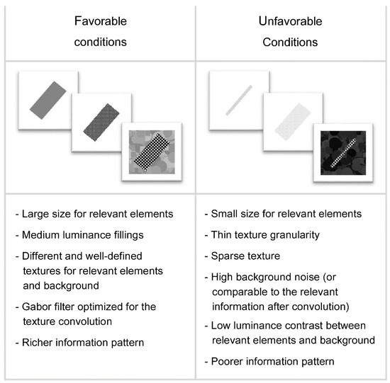
Figure 14.
Summary of results. The table summarizes the most favorable and the less favorable conditions, for a classification task performed with HMAX.
The Black Bar Image Dataset has proven to be a useful instrument of investigation, in the present assessment, creating precise test environments to respond to specific necessities, and permitting to tune and measure individual features within each image. Moreover, thanks to its modular structure, the BBID made possible a more detailed analysis of the information processing of any computational models, like HMAX.
This study, and the results obtained, naturally lead us to consider further research, which could enrich our knowledge in this field. The continuation of the in-depth analysis of HMAX, in light of the methodology introduced here, and the comparison with other functional models, could lead to new optimizations of the algorithm of Serre and colleagues. The standardized use of the Black Bar Image Dataset as a test-bench could lead to compare and analyze different functional models, from new perspectives.
The set of images of the Black Bar Image Dataset utilized in the present assessment is available at the URL: http://leadserv.u-bourgogne.fr/BBID/.
Author Contributions
A.C., O.B. and M.P. implemented the HMAX code (Matlab), and the test-set for the assessment (Matlab). A.C. and M.P. conceived and performed the assessment. A.C. and M.P. wrote the manuscript. All authors have read and agreed to the published version of the manuscript.
Funding
This work was funded by a grant from the French National Research Agency, ANR-12-INSE-0009, IRIS Project; and a grant from the ‘Conseil Régional Bourgogne Franche Comté, COGSTIM Project.
Conflicts of Interest
The authors declare no conflict of interest.
References
- Riesenhuber, M.; Poggio, T. Hierarchical models of object recognition in cortex. Nat. Neurosci. 1999, 2, 1019–1025. [Google Scholar] [CrossRef] [PubMed]
- Serre, T.; Wolf, L.; Bileschi, S.; Riesenhuber, M.; Poggio, T. Robust object recognition with cortex-like mechanisms. IEEE Trans. Pattern Anal. Mach. Intell. 2007, 29, 411–426. [Google Scholar] [CrossRef] [PubMed]
- Arbib, M.A.; Bonaiuto, J.J. From Neuron to Cognition via Computational Neuroscience; MIT Press: Cambridge, MA, USA, 2016; ISBN 0262034964. [Google Scholar]
- Serre, T.; Oliva, A.; Poggio, T. A feedforward architecture accounts for rapid categorization. PNAS 2007, 104, 6424–6429. [Google Scholar] [CrossRef] [PubMed]
- Hubel, D.H.; Wiesel, T.N. Receptive fields and functional architecture of monkey striate cortex. J. Physiol. 1968, 195, 215–243. [Google Scholar] [CrossRef]
- Serre, T.; Wolf, L.; Poggio, T. Object recognition with features inspired by visual cortex. In Proceedings of the 2005 IEEE Computer Society Conference on Computer Vision and Pattern Recognition (CVPR’05), San Diego, CA, USA, 20–25 June 2005; Volume 2, pp. 994–1000. [Google Scholar]
- Li, Y.; Wu, W.; Zhang, B.; Li, F. Enhanced HMAX model with feedforward feature learning for multiclass categorization. Front. Comput. Neurosci. 2015, 9, 1–14. [Google Scholar] [CrossRef]
- Wang, Y.; Deng, L. Modeling object recognition in visual cortex using multiple firing k-means and non-negative sparse coding. Signal Process. 2016, 124, 198–209. [Google Scholar] [CrossRef]
- Theriault, C.; Thome, N.; Cord, M. Extended coding and pooling in the HMAX model. IEEE Trans. Image Process. 2013, 22, 764–777. [Google Scholar] [CrossRef]
- Hu, X.; Zhang, J.; Li, J.; Zhang, B. Sparsity-regularized HMAX for visual recognition. PLoS ONE 2014, 9, e81813. [Google Scholar] [CrossRef]
- Lau, K.H.; Tay, Y.H.; Lo, F.L. A HMAX with LLC for Visual Recognition. arXiv 2015, arXiv:1502.02772. [Google Scholar]
- Liu, C.; Sun, F. HMAX model: A survey. In Proceedings of the 2015 International Joint Conference on Neural Networks (IJCNN), Killarney, Ireland, 12–17 July 2015; pp. 1–7. [Google Scholar]
- Deng, L.; Wang, Y. Bio-inspired model for object recognition based on histogram of oriented gradients. In Proceedings of the World Congress on Intelligent Control and Automation (WCICA), Guilin, China, 12–15 June 2016. [Google Scholar]
- Huang, Y.; Huang, K.; Tao, D.; Tan, T.; Li, X. Enhanced biologically inspired model for object recognition. IEEE Trans. Syst. Man Cybern. B Cybern. 2011, 41, 1668–1680. [Google Scholar] [CrossRef]
- Theriault, C.; Thome, N.; Cord, M. HMAX-S: Deep scale representation for biologically inspired image categorization. In Proceedings of the 2011 18th IEEE International Conference on Image Processing, Brussels, Belgium, 11–14 September 2011; pp. 1261–1264. [Google Scholar]
- Masquelier, T.; Thorpe, S.J. Unsupervised learning of visual features through spike timing dependent plasticity. PLoS Comput. Biol. 2007, 3, e31. [Google Scholar] [CrossRef] [PubMed]
- Mutch, J.; Lowe, D.G. Multiclass object recognition using sparse, localized features. In Proceedings of the 2006 IEEE Computer Society Conference on Computer Vision and Pattern Recognition (CVPR’06), New York, NY, USA, 17–22 June 2006; pp. 11–18. [Google Scholar]
- Yang, B.; Zhou, L.; Deng, Z. C-HMAX: Artificial cognitive model inspired by the color vision mechanism of the human brain. Tsinghua Sci. Technol. 2013, 18, 51–56. [Google Scholar] [CrossRef]
- Mishra, P.; Jenkins, B.K. Hierarchical model for object recognition based on natural-stimuli adapted filters. In Proceedings of the 2010 IEEE International Conference on Acoustics, Speech and Signal Processing, Dallas, TX, USA, 14–19 March 2010. [Google Scholar] [CrossRef]
- Thomure, M.D. The Role of Prototype Learning in Hierarchical Models of Vision. Ph.D. Thesis, Portland State University, Portland, OR, USA, 2014. [Google Scholar]
- Jalali, S.; Tan, C.; Ong, S.; Seekings, P.J.; Taylor, E. A encoding co-occurrence of features in the HMAX model. CogSci 2013, 2013, 2644–2649. [Google Scholar]
- Hubel, D.H.; Wiesel, T.N. Receptive fields, binocular interaction and functional architecture in the cat’s visual cortex. J. Physiol. 1962, 160, 54–106. [Google Scholar] [CrossRef] [PubMed]
- Wu, L.; Wang, Y.; Li, X.; Gao, J. Deep attention-based spatially recursive networks for fine-grained visual recognition. IEEE Trans. Cybern. 2018, 49, 1791–1802. [Google Scholar] [CrossRef] [PubMed]
- Kuang, Z.; Yu, J.; Li, Z.; Zhang, B.; Fan, J. Integrating multi-level deep learning and concept ontology for large-scale visual recognition. Pattern Recognit. 2018, 78. [Google Scholar] [CrossRef]
- Wang, Q.; Chen, K. Zero-Shot visual recognition via bidirectional latent embedding. Int. J. Comput. Vis. 2017. Available online: https://arxiv.org/pdf/1607.02104.pdf (accessed on 10 February 2020). [CrossRef]
- Rolls, E.T. Invariant visual object and face recognition: Neural and computational bases, and a model, VisNet. Front. Comput. Neurosci. 2012, 6, 35. [Google Scholar] [CrossRef]
- Serre, T.; Poggio, T. A neuromorphic approach to computer vision. Commun. ACM 2010, 53, 54–61. [Google Scholar] [CrossRef]
- Moreno, P.; Marin-Jimenez, M.; Bernardino, A.; Santos-Victor, J.; de la Blanca, N. A comparative study of local descriptors for object category recognition: {SIFT} vs {HMAX}. In Pattern Recognition and Image Analysis; Springer: Berlin/Heidelberg, Germany, 2007; pp. 515–522. ISBN 978-3-540-72846-7. [Google Scholar]
- Hamidi, M.; Borji, A. Invariance analysis of modified C2 features: Case study-handwritten digit recognition. Mach. Vis. Appl. 2010, 21, 969–979. [Google Scholar] [CrossRef]
- Holzbach, A.; Cheng, G. A fast and scalable system for visual attention, object based attention and object recognition for humanoid robots. In Proceedings of the 2014 IEEE-RAS International Conference on Humanoid Robots, Madrid, Spain, 18–20 November 2014. [Google Scholar]
- Crouzet, S.M.; Serre, T. What are the visual features underlying rapid object recognition? Front. Psychol. 2011, 2, 326. [Google Scholar] [CrossRef] [PubMed]
- Borji, A.; Itti, L. Scene classification with a sparse set of salient regions. In Proceedings of the 2011 IEEE International Conference on Robotics and Automation, Shanghai, China, 9–13 May 2011; pp. 1902–1908. [Google Scholar]
- Kornblith, S.; Cheng, X.; Ohayon, S.; Tsao, D.Y. A network for scene processing in the macaque temporal lobe. Neuron 2013, 79, 766–781. [Google Scholar] [CrossRef] [PubMed]
- Zhang, B. Classification and identification of vehicle type and make by cortex-like image descriptor HMAX. Int. J. Comput. Vis. Robot. 2014, 4, 195. [Google Scholar] [CrossRef]
- Meyers, E.; Wolf, L. Using biologically inspired features for face processing. Int. J. Comput. Vis. 2008, 76, 93–104. [Google Scholar] [CrossRef]
- Leibo, J.Z.; Mutch, J.; Poggio, T. Why the brain separates face recognition from object recognition. Proceedings of the Advances in Neural Information Processing Systems (NIPS). 2011, pp. 1–9. Available online: http://papers.nips.cc/paper/4318-why-the-brain-separates-face-recognition-from-object-recognition.pdf (accessed on 10 February 2020).
- Lapedriza, A.; Maryn-Jimenez, M.J.; Vitria, J. Gender recognition in non controlled environments. In Proceedings of the 18th International Conference on Pattern Recognition (ICPR’06), Hong Kong, China, 20–24 August 2006; Volume 3, pp. 834–837. [Google Scholar]
- Guo, G.; Mu, G.; Fu, Y.; Huang, T.S. Human age estimation using bio-inspired features. In Proceedings of the 2009 IEEE Conference on Computer Vision and Pattern Recognition, Miami, FL, USA, 20–25 June 2009; pp. 112–119. [Google Scholar]
- Guo, G.; Dyer, C.R.; Fu, Y.; Huang, T.S. Is gender recognition affected by age? In Proceedings of the 2009 IEEE 12th International Conference on Computer Vision Workshops, ICCV Workshops, Kyoto, Japan, 27 September–4 October 2009; pp. 2032–2039. [Google Scholar]
- El Dib, M.Y.; Onsi, H.M. Human age estimation framework using different facial parts. Egypt. Inform. J. 2011, 12, 53–59. [Google Scholar] [CrossRef][Green Version]
- Griffin, G.; Holub, A.; Perona, P. Caltech-256 object category dataset. Caltech Mimeo 2007, 11, 20. [Google Scholar]
- Jegou, H.; Douze, M.; Schmid, C. Hamming embedding and weak geometry consistency for large scale image search – Extended version. Proceedings of the 10th European Conference on Computer Vision (ECCV ’08). 2008. Available online: https://hal.inria.fr/file/index/docid/548651/filename/jegou_hewgc_extended.pdf (accessed on 10 February 2020).
- Welinder, P.; Branson, S.; Mita, T.; Wah, C. Caltech-UCSD birds 200. CalTech 2010, 200, 1–15. [Google Scholar]
- Marín-Jiménez, M.J.; de la Blanca, N.P. Sharing Visual Features for Animal Categorization: An Empirical Study; Springer: Berlin/Heidelberg, Germany, 2006; pp. 13–22. [Google Scholar]
- Jain, A.K.; Farrokhnia, F. Unsupervised texture segmentation using Gabor filters. In Proceedings of the 1990 IEEE International Conference on Systems, Man, and Cybernetics Conference Proceedings, Los Angeles, CA, USA, 4–7 November 1990; pp. 14–19. [Google Scholar]
- Grigorescu, S.E.; Petkov, N.; Kruizinga, P. Comparison of texture features based on Gabor filters. IEEE Trans. Image Process. 2002, 11, 1160–1167. [Google Scholar] [CrossRef]
- Bianconi, F.; Fernández, A. Evaluation of the effects of Gabor filter parameters on texture classification. Pattern Recognit. 2007, 40, 3325–3335. [Google Scholar] [CrossRef]
- Irshad, H.; Jalali, S.; Roux, L.; Racoceanu, D.; Hwee, L.J.; Le Naour, G.; Capron, F. Automated mitosis detection using texture, SIFT features and HMAX biologically inspired approach. J. Pathol. Inform. 2013, 4, S12. [Google Scholar] [CrossRef]
- Kamarainen, J.; Kyrki, V.; Kälviäinen, H. Fundamental frequency Gabor filters for object recognition. In Proceedings of the Object recognition supported by user interaction for service robots, Quebec City, QC, Canada, 11–15 August 2002; Volume 16, pp. 628–631. [Google Scholar]
- Ji, Y.; Chang, K.H.; Hung, C.-C. Efficient edge detection and object segmentation using Gabor filters. In Proceedings of the 42nd Annual Southeast Regional Conference, Huntsville, AL, USA, 2–3 April 2004; Volume 42, p. 454. [Google Scholar] [CrossRef]


© 2020 by the authors. Licensee MDPI, Basel, Switzerland. This article is an open access article distributed under the terms and conditions of the Creative Commons Attribution (CC BY) license (http://creativecommons.org/licenses/by/4.0/).