Automated Malware Detection in Mobile App Stores Based on Robust Feature Generation

Abstract

Many Internet of Things (IoT) services are currently tracked and regulated via mobile devices, making them vulnerable to privacy attacks and exploitation by various malicious applications. Current solutions are unable to keep pace with the rapid growth of malware and are limited by low detection accuracy, long discovery time, complex implementation, and high computational costs associated with the processor speed, power, and memory. Therefore, an automated intelligence technique is necessary for detecting apps containing malware and effectively predicting cyberattacks in mobile marketplaces. In this study, a system for classifying mobile marketplaces applications using real-world datasets is proposed, which analyzes the source code to identify malicious apps. A rich feature set of application programming interface (API) calls is proposed to capture the regularities in apps containing malicious content. Two feature-selection methods—Chi-Square and ANOVA—were examined in conjunction with ten supervised machine-learning algorithms. The detection accuracy of each classifier was evaluated to identify the most reliable classifier for malware detection using various feature sets. Chi-Square was found to have a higher detection accuracy as compared to ANOVA. The proposed system achieved a detection accuracy of 98.1% with a classification time of 1.22 s. Furthermore, the proposed system required a reduced number of API calls (500 instead of 9000) to be incorporated as features.

1. Introduction

The Internet of Things (IoT) is an attractive system that connects many physical devices and logical objects with networks to expand their communication capabilities. In recent years, the IoT has gained popularity owing to technological advancements in areas such as artificial intelligence, smart home devices, application systems, and cloud computing. According to the statistics on IoT usage published in 2018 [1], the number of connected IoT devices has exceeded 17 billion globally. Mobile devices are the most prominent products in demand among physical IoT devices, with approximately 10 billion active mobile devices in use [2]. Mobile users can nowadays purchase items that generally require a physical card to, for example, pay their bills using a connected mobile device. Such portable devices have been increasingly targeted by hackers given the rapid development of the mobile market [3,4].

Malware refers to any malicious code that harms user confidentiality, integrity, or availability. A malicious app appears like a clean application but hides malicious activity in the background [5,6]. Some examples of Android malware include stealing user information (e.g., login credentials and bank account numbers), sending premium short message service (SMS) messages that cost more than the standard ones, making calls, tracking user locations, hijacking microphones, streaming videos from users’ cameras, installing adware, and encrypting personal data (e.g., images, SMS, videos, and contacts).

The majority of these malicious applications can be found in third-party markets (e.g., AppChina and Anzhi) that are managed and regulated by individuals and are neither authorized nor checked by Google. However, there have been several indications of Google’s official market, formally known as the Google Play Store, containing malicious apps that exploit the confidentiality, integrity, or availability of mobile users [7]. Allix et al. [8] demonstrated that 22% of the apps on the Play Store had been flagged as malware by at least one antivirus product, whereas 50% of the apps on AppChina had been similarly flagged. One main limitation of the marketplace is that even reputed firms such as Google are unable to thoroughly check millions of mobile applications [7]. Thus, it is imperative that malicious apps are detected before they are downloaded onto portable devices.

Innumerable applications containing a large amount of information are available in the marketplace. Therefore, it is critical to employ automated techniques such as artificial intelligence and machine learning to identify relevant patterns in the available information. Machine learning-based detection involves categorizing applications into one or more predefined groups (clean or malicious) based on their contents. The ability of a machine-learning technique to detect malware is affected by the six factors listed below:

1)

Dataset

2)

Type of features

3)

Feature-weighting scheme

4)

Feature-selection algorithm used to select the most prominent features

5)

Classification algorithm used to categorize apps as malicious or clean

6)

Classifier’s parameter values

First, samples of current real-world malware were collected to understand their full capabilities. Second, the proposed system relies on the information derived from the source code to recognize malicious applications by retrieving the prominent application programming interface (API) calls requested by the malware. Numerous studies [9,10,11,12,13,14,15,16] have suggested that API calls can indicate malicious behavior and provide a detailed evaluation of the applications under investigation. Third, Term Frequency–Inverse Document Frequency (TF–IDF) was employed as a feature-weighting technique to reduce the importance of commonly requested features and increase the importance of rarely requested features. Fourth, as selecting a subset of all the features is an important goal [17], two powerful feature-selection algorithms were used—Chi-Square and analysis of variance (ANOVA)—to choose from sets of 10 to 9000 features that contribute to malware detection. Various feature subsets were employed to compare the differences between the investigated algorithms. Fifth, identifying the classification algorithm that has the most reliable detection accuracy and speed is a key aspect. Therefore, the detection accuracy and effectiveness of each of the ten machine-learning algorithms were evaluated to identify the most powerful classifiers. Finally, a classifier’s accuracy and efficiency can be improved by adjusting the default input values. However, in this study, the ten classifiers were implemented with their default input values to enable equivalent comparisons between the classifiers.

Contributions of This Study

The main contributions of this study are:

• Robust system: A fully automated tool for classifying mobile applications as clean or malicious is presented.
• Lightweight analysis: The proposed system does not drain smartphone resources and analyzes a large set of real-world data in a reasonable time.
• Feature selection: The proposed system compares different feature-selection algorithms to reduce the feature-vector dimensions.
• Relevant features: Different numbers of features are investigated to identify the lowest number of features that can obtain optimal results, evaluated based on the detection accuracy and speed of training and testing.
• Detection rate: An empirical study of ten supervised machine algorithms indicates that the proposed tool is effective on real-world data.

The rest of this paper is organized as follows: Related/previous literature is discussed in Section 2. In Section 3, a new mobile malware-detection method is presented, including app collection, feature extraction, and feature selection. The employed classification algorithms are discussed in Section 4. Section 5 details the experimental evaluation, while Section 6 describes the detection results. The results from this study are compared to recent works in Section 7. Finally, conclusions are drawn in Section 8.

2. Related Work

Several research papers in the field of malware detection have been published over the past few years [18,19,20,21,22]. Initial research studies focused on permission-based detection, signature-based detection, system call-based detection, and sensitive API-based detection. Feature-selection algorithms such as information gain (IG), principal component analysis (PCA), Chi-Square (χ²), and analysis of variance (ANOVA) were suggested to improve the detection performance [23]. Machine-learning techniques have also been applied to automate malware detection strategies [24].

Hussein et al. [25] collected a dataset of 500 clean applications and 5774 malicious applications by applying classification algorithms to the information retrieved from static (intents and permissions) and dynamic (cryptographic API calls, data leakages, and network manipulation) analyses. Each application was executed in Droidbox, and the generated log files were collected using the emulator’s logcat. The authors applied two feature selection approaches, namely IG and PCA, to the given features to identify the features likely to produce high detection accuracies.

To test the proposed methodology, Hussein et al. combined each feature-selection algorithm (IG and PCA) with four classifiers, namely Decision Tree, Gradient Boosting, Random Forest, and Naïve Bayes, which delivered average accuracies of 95%, 95%, 94%, and 94%, respectively, following testing. The detection accuracy of the IG algorithm was found to be better than that of PCA. Similarly, in this study, two feature-selection algorithms were used—Chi-Square and ANOVA—to extract the top features (i.e., packages, classes, constructors, and methods) from various feature subsets that contribute to malware detection.

In a similar study [26], Aminordin et al. developed a framework to classify clean and malicious applications using the requested permission, sensitive API calls, and metadata. A dataset consisting of 8177 Android apps was collected from the Play Store and AndroZoo, with dex2jar and JD-GUI used to extract the source code. The framework employed IG to select the most relevant features, which required approximately 62 permissions and 20 sensitive API calls. The applications were subsequently categorized using the following machine-learning algorithms: Naïve Bayes, Support Vector Machine (SVM), Decision Tree-J48, and Random Forest. The Random Forest algorithm with a 10-fold cross-validation resulted in the best detection accuracy of 95.1%. Aminordin et al. stated (Section 5) that “This study only focuses [on] and is limited to Android apps from API [levels] 16 to 24 due to the dataset provided by AndroZoo. Furthermore, this study can be enhanced by including more threat patterns created by the malware.”

Chavan et al. [27] performed a comparative analysis of clean and malicious applications, wherein 230 permissions were extracted using Androguard from a dataset of 989 clean applications and 2657 malicious applications. It was found that 118 distinct permissions occurred in the malware samples; thus, 118-entry feature vectors were constructed, which were later reduced to 74 based on the IG algorithm. Six machine-learning algorithms were investigated, namely Decision Tree, Random Forest, Support Vector Machine, logistic model trees, AdaBoost, and an artificial neural network. The highest detection accuracy (95%) was achieved using Random Forest. The analysis of applications based only on the requested permissions can bias the analysis results, as discussed in [28,29,30]. Applications without any permissions can still access the operating system and conduct covert operations, e.g., taking pictures in the background and recording key strokes. Thus, in this study, the source code of the applications was analyzed as opposed to focusing on the permissions.

Milosevic et al. [31] focused on extracting the permissions and source code to detect malicious applications targeting the Android operating system. The authors collected an M0Droid dataset that contained 200 clean applications and 200 malicious applications. The dex2jar package was applied to the collected Dalvik executable files to obtain the Java source code. The following four experiments were performed: Permission-based clustering, permission-based classification, source code-based clustering, and source code-based classification. To test their methodology, the classification algorithms were applied to each group, resulting in a detection accuracy of 89% when the permission features were applied to the full dataset. A detection accuracy of 95.1% was achieved using the source code-based classification on 10 clean apps and 22 malicious apps. It was found that the detection accuracies of the classification algorithms were better than those of the clustering algorithms. The features obtained from the source code provided better detection accuracies compared to those obtained from the permission features. Therefore, the focus of this study was to apply various classification algorithms to identify the relevant patterns in the information derived from the source code.

In a similar study [32], a tool called PIndroid was developed to detect malicious applications. Idrees et al. examined a combination of permissions and intents to construct their detection mechanism. A dataset was collected, consisting of 445 clean applications from the Play Store, AppBrain, F-Droid, Getjar, Aptoid, and Mobango, while 1300 malicious applications were obtained from Genome, VirusTotal, The Zoo, MalShare, and VirusShare. The study focused on the top 24 of the 145 total permissions, with the permissions split into two groups—normal and dangerous. The authors extracted 135 intents from the entire dataset and found that each malicious application used two to eight intents. The Pearson correlation coefficient was used to measure the strength of the association between the permissions and intents.

Idrees et al. investigated six machine-learning algorithms—Multilayer Perceptron (MLP), Decision Table, Decision Tree, Naïve Bayesian, Random Forest, and Sequential Minimal Optimization (SMO), and obtained average detection accuracies of 99.5%, 99.6%, 99.2%, 98.8%, 98.5%, and 95.6%, respectively. Although their dataset contained only 445 clean applications and 1300 malicious applications, the majority class (1300 malicious applications) dominated the minority class (445 clean applications).

Yerima et al. [33] presented an automated approach that employed both static analyses and machine-learning algorithms to detect malevolent applications. The study found static analyses to be more advantageous than dynamic analyses; for example, static analysis can handle several evasion techniques without affecting smartphone resources. Static analyses were used to extract API calls, Linux system commands, and permissions from a dataset of 1000 malicious applications and 1000 clean applications. The authors found 25 features used by the malware samples that did not appear in the clean samples. A Bayesian classifier was applied to the extracted features, resulting in detection accuracies ranging from 89.3% to 92.1%. Yerima et al. stated (Section VI) that “We observe increasing accuracy and decreasing error rates when a larger number of features [is] used to train the classifier.” Therefore, in this study, sets of 10 to 9000 features that contribute to malware detection were investigated.

3. Experimental Design

The proposed system consists of several steps, as shown in Algorithm 1. The architecture of this system can be summarized in the following steps, which can be applied to both clean and malicious samples.

3.1. App Collection

In this section, the dataset that was used to train and evaluate the proposed system is presented. Both clean and malicious applications were required to test the proposed system. Currently, the Play Store is the main Android market available to users for downloading their applications. This market is administered by Google [34], which often checks the applications to ensure they do not contain malicious apps. Each application in the Play Store must contain a trusted digital signature for safe download by the users.

Algorithm 1

Require: D*, a set of features   Require: A*, a set of Android applications   Require: D*, a set of features   Require: C*, a set of classifiers ∈ {Naïve Bayes, Random Forest, k-NN, SMO, etc.}   Require: TD*, a set of training datasets   Require: VD*, a set of validation datasets   Require: PF, a set of variables for normalization   Require: S*, Boolean score for the respective zones: q occurs/0 does not occur   Require Labels: L = {Malicious, Clean}   For each application $A_i$ in A*:      Generate MD5, SHA1, SHA256, and SHA512 for $A_i$.      $\mathbf{Decompile} A_i$ using Androguard      Extract features D*      For each $\mathrm{feature} D_i$ $\mathrm{in} D^{\ast }$          $\mathbf{Count}\_\mathbf{freq} D_i$ ();          $\mathbf{Freq} \left[D_i\right] += \mathrm{Freq} [D_i$]          $\mathbf{PF}\leftarrow \mathrm{Pf}/\left|\mathrm{A}\ast \right|$      // normalize frequencies      End for   End for   While $p_1$ ≠ $\mathrm{Nil} \mathrm{and} {\mathit{p}}_{\mathbf{2}}$ ≠ Nil        // weighting with TF-IDF   Do if $AppI{D}_{\left(p1\right)}$ $== AppI{D}_{\left(p2\right)}$       $\mathbf{Then} \mathrm{scores} [App(I{D}_{p1})]$ $\leftarrow$ $\mathrm{weighted} \mathrm{zone} \sum _{i=1..I}\left(g_i, s_i\right)$       ${\mathit{p}}_{\mathbf{1}} \leftarrow next\left(p_1\right)$       ${\mathit{p}}_{\mathbf{2}} \leftarrow \mathrm{next}\left(p_2\right)$   Else if $App(I{D}_{p1})$ $< AppI{D}_{\left(p2\right)}$       $\mathbf{Then} p_1 \leftarrow next\left(p_1\right)$   Else  ${\mathit{p}}_{\mathbf{2}} \leftarrow \mathrm{next}\left(p_2\right)$   Return scores   For each $PF :$   // Feature selection        Select top selected features D* using ANOVA                  ${\displaystyle {\displaystyle \sum }_{i=1}^K}{n}_i{\left(\overline{Y_i}- \overline{Y}\right)}^2 / \left(K-1\right)$        Select top selected features D* using Chi-Square                  ${\displaystyle {\displaystyle \sum }_{i=1}^K}{n}_i{\left(\overline{Y_i}- \overline{Y}\right)}^2 / \left(K-1\right)$   End for   For each $\mathrm{classifier} C_i$ in C*:        $\mathbf{Train} \mathrm{classifier} ({\mathit{C}}_{\mathit{i}}, \mathit{t}{\mathit{d}}_{\mathit{i}}) // \mathrm{train} \mathrm{classifier} {\mathit{c}}_{\mathit{i}} \mathrm{with} \mathrm{the} \mathrm{training} \mathrm{samples} t{d}_i$   End for   For each $\mathrm{classifier} C_i$ in C*:        ${\mathit{r}}_{\mathit{i}}$ = classify ($C_i$, $V{D}_i$) $// \mathrm{evaluate} \mathrm{classifier} {\mathbf{c}}_{\mathit{i}}$ $\mathrm{with} \mathrm{the} \mathrm{validation} \mathrm{samples} V{D}_i$        ${\mathit{a}\mathit{p}\mathit{p}\mathit{l}\mathit{i}\mathit{c}\mathit{a}\mathit{t}\mathit{i}\mathit{o}\mathit{n}}_{\mathit{l}\mathit{a}\mathit{b}\mathit{e}\mathit{l}}.$ Add ($labe{l}_i$)   End for

In the proposed system, the first step involved the download of clean applications from the Play Store, which was performed using AndroZoo [8]. The AndroZoo project contains millions of Android applications collected from several sources (e.g., Play Store, PlayDrone, Anzhi, and AppChina). At the time of writing, 7,819,669 apps were available for download from the Play Store market using the AndroZoo project [35]. Using the az script, 19,000 clean applications were collected from the Play Store. Furthermore, 17,915 malware samples were collected from VirusTotal, AndroZoo, the Zoo, MalShare, and Contagio mobile.

Allix et al. [36] reported that the Play Store market might contain malware applications. Hence, VirusTotal was used to scan the entire dataset of malware and clean applications used in this study, wherein 70 anti-virus tools scrutinized each application to classify it as clean or malicious. Only those malware samples that were identified as being malware by at least ten anti-virus companies were selected. If any one of the 70 engine outputs identified an application as ‘malicious,’ it was marked as malware and removed from the dataset. The samples were then divided into two sets, namely the training and validation sets. The training set assists in building a new scheme based on the patterns and structures learned from a large proportion of the data, while the validation set tests the resulting scheme on data never seen by the classifier.

3.2. Feature Extraction

The next step involved extracting information from the entire dataset via static analysis using Androguard [37]. Androguard parses the byte codes of Dalvik executable files and then transforms the contents into a human-readable format. Various items, namely packages, classes, constructors, methods, and fields, were extracted from the source code. The resulting data were stored in log files so that scikit-learn could be used to generate the feature vectors for each application based on its API calls [38]. Thus, each feature vector had 27,253 distinct features. The Term Frequency calculates the number of occurrences of each feature in an application and subsequently divides it by the total number of features.

The next step involved reducing the weights corresponding to the features that occur in many applications. The TF–IDF method, which is a well-known weighting method [39], was applied to normalize the entries in the value vectors. TF means term-frequency, which calculates the number of occurrences of each feature in an application and divides it by the total number of features. Inverse Document Frequency (IDF) measures the importance of a feature by comparing its frequency of occurrence to those in other applications. TF–IDF is one of the best-known measures for specifying the weights [40]. The main objective of employing TF–IDF, as opposed to measuring the number of appearances, is to reduce the weight of features that appear frequently in many samples and increase the weight of features that appear less frequently in a small part of the training corpus. TF–IDF can be computed as

$$tf\ast idf= \sqrt{\frac{n_{ij}}{{{\displaystyle \sum }}_k{n}_{kj}}}\ast \ln \left[\frac{\left|D\right|}{d_j : t_i d_j+1}\right]$$

(1)

where $n_{ij}$ is the number of appearances of feature $t_i$ in application $d_j$, and the denominator is the number of appearances of all the features in application $d_j$. $\left|D\right|$ is the total number of applications in the dataset, and $d_j : t_i d_j+1$ is the application frequency, i.e., the number of applications in which feature $t_i$ appears.

3.3. Feature Selection Metrics

Some features might provide limited information on the actual contents of malicious applications to the classifier [41,42]. The imperative goals of any malware-detection system include the identification of a subset of features from the entire feature set, with subsequent reduction in the high data dimensionality. In practice, the main purpose of feature selection is the selection of valuable features from the total number of features, leading to improved detection performance and reduced computation time. Therefore, in this study, the focus was on reducing the number of features to identify the most valuable information for classification algorithms, while simultaneously discarding any irrelevant, redundant, or noisy features.

In this study, two feature selection methods, namely Chi-Square and ANOVA, were used to evaluate the performance of the proposed system. Chen et al. [43] reported that ANOVA solved the problem of imbalanced data and improved the stability and reliability of their proposed training model. ANOVA searches for the existence of important variances in the dependent variable values, whereas Chi-Square searches for relevant features among the malware class.

3.3.1. Analysis of Variance (F-Value)

The analysis of variance (F-value) was applied to the sets of 10 to 9000 features to select the features with the highest scores. This metric measures similarities between the relevant features and reduces the scale of the feature vector between the two groups (malware and clean apps). Calvert and Khoshgoftaar [44] reported ANOVA to be an efficient algorithm for measuring the similarity of relevant features, reducing the high dimensionality of the features, and improving the detection accuracy. The mathematical definition of ANOVA can be expressed as

$${\displaystyle \sum }_{i=1}^K{n}_i{\left(\overline{Y_i}- \overline{Y}\right)}^2 / \left(K-1\right),$$

(2)

where $\overline{Y_i}$ denotes the sample mean in the i^th group, $n_i$ is the number of observations in the i^th group, $\overline{Y}$ denotes the overall mean of the dataset, and $K$ denotes the number of groups.

3.3.2. Chi-Square

Chi-Square is a statistical test that measures the similarity between the expected and actual model results. It is valuable for recognizing the relationships between the categorical variables. Chi-Square was applied to each feature to select the highest scores from the sets of 10 to 9000 features. The mathematical definition of Chi-Square is given by

$$x^2= {\displaystyle \sum }\frac{{\left(O_i-E_i\right)}^2}{E_i},$$

(3)

where $O$ is the observed (actual) value and $E$ is the expected value.

4. Classification-Based Malware Detection

Data mining-based malware detection algorithms can be divided into two main groups: classification and clustering. In classification algorithms, the datasets are known to the user and input to the classifier in advance for training. The datasets are divided into classes $\left(x_1, y_1\right), \left(x_2,y_2\right),\dots \left(x_n, y_n\right)$, where $x_i$ is the $i_{th}$ data point (application) and $y_i$ is the target class (malicious or clean). The model will then be generated during dataset training. The objective of the above-mentioned process is to develop a classifier that can automatically categorize mobile applications as clean or malicious and identify mobile malware variants. In contrast, in clustering algorithms, the objective is to separate groups with similar characteristics and allocate them to clusters without training the dataset.

In this study, various classification algorithms were employed to identify the pattern of malicious applications, as referenced in [31]. The authors have stated (in Section 4) that “Clustering and unsupervised learning methods are worse for predicting whether [an] application is malicious or not, since they base their learning on similarities between different instances.” This study discussed the detailed implementations of ten supervised-learning algorithms, namely Naïve Bayes, k-Nearest Neighbors, Random Forest, J48, SMO, Logistic Regressions, the AdaBoost decision-stump model, Random Committee, JRip, and Simple Logistics. These algorithms were compared using a real-world dataset.

Naïve Bayes is considered a simple probabilistic classifier because it incorporates a straightforward model for representing the data, learning, and prediction classes [12,45]. Naïve Bayes determines a specific class without making any connections to the other features by assuming that all the features are independent, with no attribute hidden within the given features. The authors in [25,31,46,47] obtained high detection results by applying the Naïve Bayes classifier to Android malware. The task of the Naïve Bayes classifier is to adequately predict whether an application is clean or malicious based on the assumption that all of the features are conditional on the class label. The class can be computed as follows:

$$p\left(\mathrm{w}\right|\mathrm{c}, \varphi )={\displaystyle \prod }_{\mathrm{i}=1}^{\mathrm{D}}p( w_i|c, {\varphi }_{ic}),$$

(4)

where $\mathrm{D}$ is the feature vector ($w_1$,$w_2$,…,$w_{\mathrm{D}}$) and ${\varphi }_{ic}$∈$\varphi$ is a maximum-likelihood estimate of the feature in class c.

K-Nearest Neighbors (k-NN) is a simple classification algorithm that attempts to interpret the output, time, and accuracy. It has been employed in various fields, such as health, finance, education, text data, face recognition, and malware detection. The k-NN algorithm uses less information than other data distributions or no prior information. In the k-NN algorithm, the constant “K” represents the number of nearest neighbors of a test data point. The prediction value is then calculated when all the data points predict the class of the test data point. The task of the nearest-neighbors algorithm is to identify the similarities or differences using various distance metrics such as the Chebyshev metric, city-block distance, Euclidean distance, cosine distance, Minkowski distance, and Manhattan distance.

In this study, the Euclidean distance of an application’s features from the feature space was employed while training the samples. To determine the distance between the query point ($x$) and all the training samples $x_i^j$, the Euclidean distance can be computed as follows:

$$d(x,x_i^j)\sqrt{{\displaystyle \sum }_{i=1}^{d}x\left(i\right)-x_i^j}{(i)}^2.$$

(5)

The weighted distance of the test data from the closest point can be computed as follows:

$$w( x_i, x_i^j)=1- \frac{d\left(x_i, x_i^j\right)}{{{\displaystyle \sum }}_{i=0}^{k}d\left(x_i, x_i^j\right)}.$$

(6)

Sequential Minimal Optimization (SMO) is a fast implementation of a Support Vector Machine (SVM), which is based on statistics theory. The main challenge with the SVM is that the parameters (also known as hyper parameters) must be carefully selected while training the samples. Therefore, the excessive operational costs of the search for a predefined set of parameter values have led to new optimization algorithms being investigated. SMO can be used to solve controlled learning process problems without using extra storage or optimizing the numerical parameter values. SMO constructs a set of hyper-planes in an n-dimensional space that can be used for classification. The algorithm breaks the optimization problem into a series of sub-problems that can be analytically solved later. The SMO model can be computed as follows:

$$\mathrm{f}\left(\mathrm{x}, \mathsf{\alpha }\right){\displaystyle \sum }_{\mathrm{i}=1}^{\mathrm{N}}({\mathsf{\alpha }}_{\mathrm{i}}^{\ast }-{ \mathsf{\alpha }}_{\mathrm{i}}) \mathrm{K} \left({\mathrm{x}}_{\mathrm{i}}.{\mathrm{x}}_{\mathrm{j}}\right)+\mathrm{b},$$

(7)

where ${\alpha }_1$ and ${\alpha }_2$ are two Lagrange multipliers and $k$ is the kernel function. The kernel function can have various functional forms, as shown in

Table 1. Kernel functions used in Sequential Minimal Optimization (SMO).

Kernels	Formula	Parameters
Polynomial Kernel	$\mathrm{K} \left({\mathrm{x}}_i.{\mathrm{x}}_j\right)= {\left({\mathrm{x}}_i.{\mathrm{x}}_j+\mathrm{k}\right)}^{\mathrm{d}}$	K: Constant	(8)
Normalized Polynomial Kernel	$\mathrm{K} \left({\mathrm{x}}_i.{\mathrm{x}}_j\right)= \frac{{\left(\left({\mathrm{x}}_i \ast {\mathrm{x}}_j\right)+1\right)}^d}{\sqrt{{\left(\left({\mathrm{x}}_i \ast {\mathrm{x}}_j\right)+1\right)}^d {\left(\left({\mathrm{x}}_j \ast {\mathrm{x}}_j\right)+1\right)}^d}}$	d: Degree of polynomial	(9)
PUK	$\mathrm{K}\left({\mathrm{x}}_i.{\mathrm{x}}_j\right)=\frac{1}{{\left[1+{\left(\frac{2 \ast \sqrt{ {\Vert \left({\mathrm{x}}_i-{\mathrm{x}}_j\right)\Vert }^2 \sqrt{2^{\left(1/\mathrm{w}\right)}-1}} }{\mathsf{\sigma }}\right)}^2\right]}^w}$	$w, \mathsf{\sigma }$: Pearson width parameters	(10)
RBF	$\mathrm{K} \left({\mathrm{x}}_i.{\mathrm{x}}_j\right)=\exp (-\Vert {\mathrm{x}}_i,{\mathrm{x}}_j\Vert / {\left(2\mathsf{\gamma }\right)}^2$	γ: Kernel dimension	(11)

.

SMO attempts to map the data points from an n-dimensional input space to a high-dimensional vector space, as it is easier to solve the algorithm in the feature space. The mapping is performed by selecting the best kernel functions, such as a polynomial kernel, normalized polynomial kernel, Pearson VII function-based universal kernel (PUK), and radial basis function kernel (RBF). SMO with the four kernels presented in Table 1 was implemented.

Random Forest is an ensemble of decision trees that uses the training data to learn to make predictions. Random Forest is a powerful classifier as it (1) expresses rule sets that humans can easily understand, (2) can handle high-dimensional data, (3) delivers better performance than a single tree classifier, (4) handles non-linear numeric and categorical predictors, (5) can calculate the variable importance for the classifier, (6) can select an attribute that is most useful for prediction, and (7) does not require the data to be rescaled or transformed. The algorithm constructs many individual decision trees while training the dataset. The prediction for the unseen data is then generated by collecting the most/maximum votes for a classification or the average votes from all the individual regression trees on x for a regression.

$$\hat{f}=\frac{1}{B} {\displaystyle \sum }_{b=1}^B{f}_b\left({\mathrm{x}}^{\prime }\right).$$

(12)

The standard deviation of all the individual regressions on x’ can be calculated for the prediction uncertainty as follows:

$$\mathsf{\sigma }=\sqrt{\frac{{{\displaystyle \sum }}_{b=1}^B{\left(f_b\left({\mathrm{x}}^{\prime }\right)-\hat{f}\right)}^2}{B-1}}.$$

(13)

J48 is a non-parametric classifier based on the Decision Tree, which is used for classification and regression. The task of a decision tree is to construct a model that predicts the value of a target variable by learning simple decision rules that operate on different conditions as compared to the feature vector. The J48 classifier has been implemented in various research areas such as bioinformatics, academic performance, network-intrusion detection, image processing, finding active objects, e-governance, soil fertility, crime prediction, and road traffic monitoring. In a decision tree, the binary search starts from the root and progresses downward through the tree until it reaches a leaf node. The Decision Tree converts the trained trees into sets of if-then rules based on the characteristics corresponding to the decision trees while training the dataset. When the data instances match the category conditions, that branch is terminated and assigned the target value. When a target is a classification outcome taking on the values 0 and 1, for a node m, representing a region $r_m$ with observations $N_m$, the proportion of class $k$ observations in the node can be calculated as follows:

$$p_{mk}=\frac{1}{N_m {{\displaystyle \sum }}_{x_i{R}_m}I\left(y_i=k\right)}.$$

(14)

Three impurity measures are commonly used in binary decision trees, as shown in

Table 2. Impurity measures in decision trees.

Impurity Measure	FORMULA
Entropy	$H(X_m)={\displaystyle \sum }_k{p}_{mk}\log (p_{mk})$	(15)
Gini	$H(X_m)={\displaystyle \sum }_k{p}_{mk}(1-p_{mk})$	(16)
Classification Error	$H(X_m)=1-\max \left(p_{mk}\right)$	(17)
Parameters	$X_m$ is the training data in node $m$

.

Logistic Regression is a regression technique used for predicting the outcome of a categorical dependent variable; hence, it can have only two values: 0 or 1, in this case. It has been widely used in statistics to measure the probability of occurrence of a certain event, based on previous data, by specifying the category with which it most closely aligns. This algorithm can predict a new data point from the feature space with probability predictions using a linear function, followed by a logistic function. The linear function of the predictor variables is calculated and the result is run through a link function. Conditional probability can be modeled as

$$p_w\left(y=\pm 1|x\right)=\frac{1}{1+e^{-y{w}^{t}x\prime }},$$

(18)

where $\mathrm{x}$ is the data, $y$ is the class label (malware, clean), and $\mathrm{w}{R}_n$ is the weight vector.

AdaBoost is one of the most common boosting algorithms in ensemble learning, and is short for Adaptive Boosting. This algorithm can be used in conjunction with many other machine-learning algorithms to improve the detection accuracy. AdaBoost supports a weight distribution over the training set to minimize errors and maximize the margin in terms of the features. It can generate effective and accurate predictions by combining many simple and moderately accurate hypotheses into a strong hypothesis. AdaBoostM1 is one of the two major versions of AdaBoost algorithms for binary-classification problems. All the results presented in this paper were obtained by applying AdaBoostM1 in conjunction with the decision-stump model, which consists of a one-level decision tree.

Random Committee is a supervised machine-learning algorithm, which is a form of ensemble learning. It is based on the assumption that the detection accuracy can be improved by combining different machine-learning algorithms. Each base classifier is built using the training data from a different random number of seeds. The final prediction is calculated by averaging the predictions generated by each of these individual base classifiers. All the results presented in this paper were obtained by applying the Random Committee algorithm in conjunction with the Random Tree model, which constructs a tree that considers K features randomly chosen at each node.

JRip is an inference and rule-based learner that implements a propositional rule learner, Repeated Incremental Pruning to Produce Error Reduction (RIPPER). JRip works in two phases, first growing and then pruning to avoid over-fitting. One rule predicts the target class for each feature and subsequently selects the most informative features with fewer errors to build the algorithm. A one-level tree is then generated. The information gain is used to indicate the antecedent, and Reduced Error Pruning (REP), along with the accuracy metric, is used to prune the rule.

Simple Logistics is one of the most popular machine-learning algorithms, as it is very accurate and compact compared to the other classifiers. This algorithm has been implemented in various research fields such as emotions from human speech recognition, diabetes diagnosis, text classification, financial analysis, soybean-disease diagnosis, and student academic result prediction. Simple Logistics builds linear logistic regression models. LogitBoost is used to fit the logistic models with simple regression functions as base learners. The optimal number of iterations to be performed by LogitBoost is cross-validated, resulting in automatic attribute selection.

5. Performance Evaluation Metrics

K-fold cross-validation, which is a popular technique for estimating the performance of a predictive model based on the given features, was adopted in the training and testing phases. The purpose of K-fold cross-validation is to indicate how well the classifier performs when asked for new predictions about an application that it has never seen. The K-fold method separates the given dataset into two subsets; the first is used to test the model, while the remaining K-1 subsets are used to train the model. After a model has been processed using the training set, the model can be tested by making predictions against the validation set. When the K value is small, the model has a small amount of data to learn from. Conversely, when the K value is large, the model has a much better chance of learning all the relevant information in the training set. The benefit of cross-validation over repeated random subsampling is that all observations are used for both training and testing, and each observation is used exactly once for validation. In this study, a 10-fold cross-validation was performed for all the datasets.

All results in this paper include the F-measure, as it equally combines precision and recall into a single number for evaluating the performance of the entire system.

Precision: This is defined as the number of predictions made that is actually correct or relevant out of all the predictions based on the positive class, and can be computed as follows:

$$\mathit{P}\mathit{r}\mathit{e}\mathit{c}\mathit{i}\mathit{s}\mathit{i}\mathit{o}\mathit{n}= TP/\left(TP+FP\right).$$

(19)

Recall: This is defined as the sensitivity corresponding to the most relevant result, and can be computed as follows:

$$\mathit{R}\mathit{e}\mathit{c}\mathit{a}\mathit{l}\mathit{l}= TP/\left(TP+FN\right).$$

(20)

F-Measure: The combination of precision and recall can be computed as follows:

$$\mathit{F}-\mathit{M}\mathit{e}\mathit{a}\mathit{s}\mathit{u}\mathit{r}\mathit{e}=2 \ast \frac{Precision\ast Recall}{Precision+Recall}.$$

(21)

6. Results

To evaluate the performance, reliability, and efficiency of the proposed system, two representative feature-selection algorithms with ten different classifiers were evaluated to select the best features and achieve high detection accuracy. The first feature-selection algorithm employed was chi-square, which searches for the relevant features; the second algorithm was ANOVA, which searches for the existence of important variances in the dependent variable values. The performance and efficiency of the corresponding feature sets were subsequently compared.

In this study, sets of 10 to 9000 features that were used as relevant features were selected, and several experiments were conducted using ten different machine-learning algorithms. The number of features selected by Chi-Square and ANOVA was set to 10, 25, 50, 100, 200, 300, 500, 1000, 3000, 5000, 7000, and 9000. Each set was then used for training and testing the ten machine-learning algorithms. The previously detailed feature ranking and classification algorithms were executed via ten-fold cross-validation experiments for each selected feature set.

The standard measure of success in machine learning is the classifier performance. This involves comparing the effectiveness of the different classifiers on different feature subsets, and then measuring how efficiently the results were generated for the different feature subsets. To validate the quality of a selected feature subset, the F-measure was used to measure the classifier’s effectiveness, while the total time taken for training and testing was reported. The highest classification performance values for each feature-subset size are marked in bold typeface.

Table 3. Ranking of the features according to their importance in ANOVA.

Feature Name	Rank
Landroid/content/Context;->getResources()Landroid/content/res/Resources	1
Landroid/view/View;->findViewById(I)Landroid/view/View	2
Landroid/view/View;->setVisibility(I)V	3
Ljava/lang/Enum;-><init>(Ljava/lang/String; I)V’	4
Ljava/lang/Enum;->valueOf(Ljava/lang/Class; Ljava/lang/String;)Ljava/lang/Enum;’	5
Ljava/lang/Math;->min(I I)I’	6
Ljava/util/HashSet;-><init>()V	7
Ljava/util/Iterator;->hasNext()Z	8
Ljava/util/Iterator;->next()Ljava/lang/Object; numeric	9
Ljava/util/Map;->clear()V numeric	10

displays the relative importance of various features, as measured by ANOVA, when the entire dataset was trained. Owing to space limitations, the table only lists the best ten features. The getResources-related features are of higher importance, followed by the findViewById-based features and setVisibility.

Table 4. Ranking of the features according to their importance in Chi-Square.

Feature Name	Rank
java/javax/mmmmm;->sendTextMessage(Ljava/lang/String;Ljava/lang/String; Ljava/lang/String; Landroid/app/PendingIntent; Landroid/app/PendingIntent;)V	1
Landroid/util/Pair;-><init>(Ljava/lang/Object; Ljava/lang/Object;)V	2
Landroid/view/View;->findViewById(I)Landroid/view/View;	3
Ljava/lang/Character;-><init>(C)V	4
Ljava/lang/Class;->getMethod(Ljava/lang/String; Ljava/lang/Class;)Ljava/lang/reflect/Method;	5
Ljava/lang/StringBuilder;-><init>()V	6
Ljava/lang/StringBuilder;->append(Ljava/lang/String;)Ljava/lang/StringBuilder;	7
Ljava/lang/reflect/Method;->invoke(Ljava/lang/Object; Ljava/lang/Object;)Ljava/lang/Object;	8
Ljava/util/Hashtable;->puut(Ljava/lang/Object; Ljava/lang/Object;)Ljava/lang/Object;	9
Ljava/util/Vector;->elementAt(I)Ljava/lang/Object;	10

displays the relative importance of various features, as measured by chi-square, when trained using the entire dataset. Owing to space limitations, the table only lists the ten best features. The sendTextMessage-related features were found to be of greater importance, followed by the Pair-based features and findViewById.

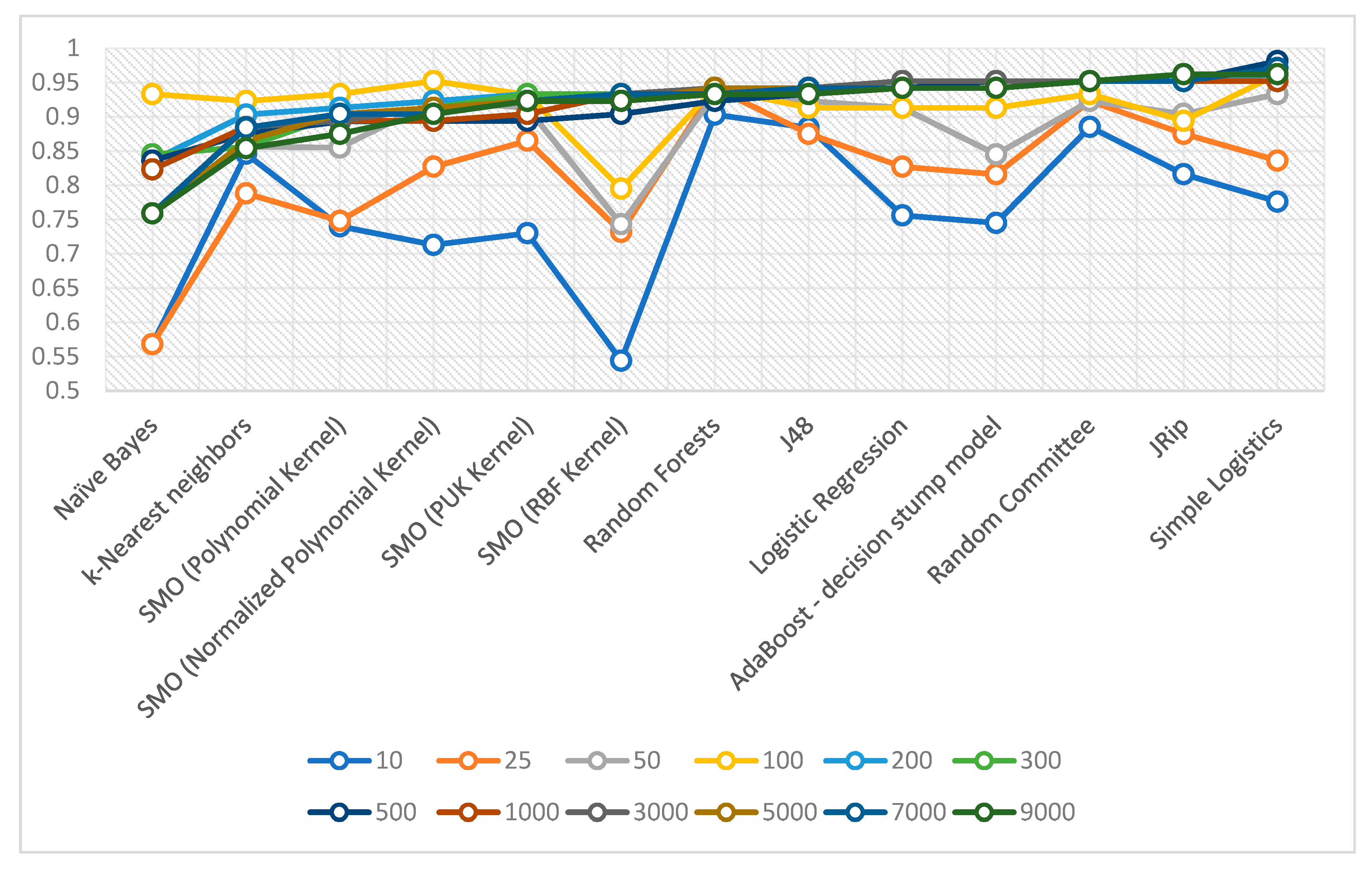
6.1. Detection Accuracy Using ANOVA-Based Feature Selection

Figure 1 and

Table 5. Detection Accuracy with ANOVA Feature Selection According to the Feature Size.

Algorithm	10	25	50	100	200	300	500	1000	3000	5000	7000	9000
Naïve Bayes	0.729	0.807	0.798	0.836	0.826	0.865	0.835	0.874	0.923	0.913	0.913	0.913
k-Nearest neighbors	0.865	0.913	0.904	0.904	0.904	0.904	0.894	0.923	0.933	0.855	0.815	0.814
SMO (Polynomial Kernel)	0.817	0.817	0.855	0.884	0.894	0.904	0.933	0.942	0.962	0.952	0.962	0.952
SMO (NormalizedPolynomial Kernel)	0.798	0.885	0.894	0.923	0.942	0.933	0.942	0.932	0.932	0.923	0.932	0.923
SMO (PUK Kernel)	0.875	0.904	0.933	0.932	0.903	0.874	0.864	0.844	0.774	0.763	0.774	0.772
SMO (RBF Kernel)	0.695	0.702	0.73	0.827	0.846	0.836	0.865	0.904	0.913	0.904	0.894	0.885
Random Forests	0.846	0.904	0.942	0.952	0.952	0.942	0.952	0.933	0.942	0.942	0.942	0.942
J48	0.836	0.894	0.846	0.885	0.855	0.923	0.904	0.904	0.923	0.923	0.942	0.933
Logistic Regression	0.798	0.817	0.894	0.933	0.904	0.837	0.865	0.817	0.952	0.971	0.952	0.904
AdaBoost–decision stump model	0.827	0.837	0.874	0.875	0.836	0.933	0.942	0.913	0.933	0.933	0.962	0.962
Random Committee	0.846	0.913	0.904	0.942	0.923	0.971	0.933	0.933	0.942	0.952	0.942	0.942
JRip	0.817	0.856	0.904	0.904	0.894	0.904	0.971	0.884	0.904	0.933	0.913	0.933
Simple Logistics	0.817	0.808	0.923	0.923	0.923	0.933	0.942	0.923	0.942	0.923	0.913	0.923

show the weighted-average detection accuracy results for all ten classifiers with different feature subset sizes selected by ANOVA: 10, 25, 50, 100, 200, 300, 500, 1000, 3000, 5000, 7000, and 9000. As shown in the table, the average detection results improved as the number of selected features increased. The best detection result of 97.1% was obtained using the following three classifiers: Random Committee with 300 sets, JRip with 500 sets, and Logistic Regression with 5000 sets. The SMO (RBF kernel) algorithm was less effective than the other selected machine-learning algorithms for Android malware detection based on the selected features.

As shown in Table 5, the highest detection accuracy was achieved when using sets of 300, 500, and 5000. As identical results were achieved for each of the sets, the training and testing speeds corresponding to each of the sets with the best results (Figure 2) were also tested. The Random Committee, JRip, and Logistic Regression classifiers required 0.04, 0.268, and 0.541 s, respectively, for training and testing the dataset with 300 features. For the dataset with 500 features, the Random Committee, JRip, and Logistic Regression classifiers took 0.058, 0.664, and 1.418 s, respectively, while 0.084, 1.166, and 3.843 s, respectively, were required for the dataset with 1000 features.

As shown in Figure 2, not only did the Random Committee classifier perform superior detection, but the time taken to train and test was also very fast. Hence, this indicates that Random Committee proved to be the most reliable classifier, with an F-measure of 97.1% and time of 0.04 s for training and testing the dataset.

6.2. Detection Accuracy Using Chi-Square-Based Feature Selection

Figure 3 and

Table 6. Detection Accuracy with Chi-Square Feature Selection According to the Feature Size.

Algorithm	10	25	50	100	200	300	500	1000	3000	5000	7000	9000
Naïve Bayes	0.568	0.568	0.759	0.933	0.836	0.845	0.836	0.823	0.759	0.759	0.759	0.759
k-Nearest neighbors	0.846	0.788	0.856	0.923	0.903	0.856	0.875	0.885	0.885	0.865	0.884	0.854
SMO (Polynomial Kernel)	0.74	0.748	0.855	0.933	0.913	0.904	0.893	0.894	0.894	0.904	0.904	0.875
SMO (NormalizedPolynomial Kernel)	0.713	0.827	0.923	0.952	0.923	0.913	0.894	0.894	0.913	0.913	0.904	0.904
SMO (PUK Kernel)	0.73	0.865	0.913	0.932	0.933	0.933	0.894	0.904	0.923	0.923	0.923	0.923
SMO (RBF Kernel)	0.544	0.732	0.743	0.795	0.933	0.933	0.904	0.933	0.933	0.923	0.933	0.923
Random Forests	0.903	0.942	0.933	0.942	0.933	0.942	0.923	0.933	0.942	0.942	0.933	0.933
J48	0.884	0.875	0.923	0.913	0.942	0.942	0.933	0.942	0.942	0.942	0.942	0.933
Logistic Regression	0.756	0.827	0.913	0.913	0.942	0.952	0.942	0.952	0.952	0.942	0.942	0.942
AdaBoost–decision stump model	0.745	0.816	0.845	0.913	0.942	0.952	0.952	0.952	0.952	0.942	0.942	0.942
Random Committee	0.885	0.923	0.923	0.933	0.952	0.952	0.952	0.952	0.952	0.952	0.952	0.952
JRip	0.816	0.875	0.904	0.894	0.952	0.962	0.952	0.952	0.952	0.952	0.952	0.962
Simple Logistics	0.776	0.836	0.933	0.962	0.962	0.962	0.981	0.952	0.971	0.971	0.971	0.962

present the weighted-average detection-accuracy results for all ten classifiers with different feature subset sizes selected by chi-square: 10, 25, 50, 100, 200, 300, 500, 1000, 3000, 5000, 7000, and 9000. As shown in the table, the average detection results improved as the number of selected features increased. This indicates that the SMO (RBF kernel) algorithm was less effective than the other selected machine-learning algorithms for Android malware detection. The best detection result of 98.1% was obtained using Simple Logistics, followed by the AdaBoost–decision stump model, Random Committee, and JRip, which achieved a 95.2% detection accuracy with 500 sets.

The speeds for training and testing the dataset with 500 features were tested/evaluated, as shown in Figure 4. The fastest algorithm was Naïve Bayes, requiring 0.04 s with a detection accuracy of 83.6%, followed by Random Committee and k-NN, requiring 0.055 s with a 95.2% detection accuracy and 0.105 s with an 87.5% detection accuracy, respectively.

7. Discussion

In this section, the proposed system will be compared to state-of-the-art systems for mobile malware detection using the following standard metrics: Dataset, feature type, feature-selection algorithms, number of features used in the experiment, overall detection performance, and speed of training and validating the system. To highlight the performance and efficiency of the current work, a useful comparison has been provided in

Table 7. Comparison between the proposed system and state-of-the-art systems.

Ref	Dataset	Feature Type	Feature Selection	# of Features	Machine Learning	Accuracy	Speed
[1]	Mal = 2925 Clean = 3938	Combined app attributes and Permission features (CAPF)	IG	20 50	1. Naïve Bayes 2. Simple logistic 3. Decision tree, 4. Random tree	97.5%	6.41 s
[2]	Mal = 250 Clean = 250	Static feature and dynamic features	?	202	1. SVM 2. C4.5 3. Naive Bayes 4. LR 5. MLP 6. Deep Learning	96.5%	?
[3]	Apps = 50,000	CFGs	IG	50, 250 500, 1000, 1500, 5000	1. Random Forest 2. J48, 3. JRip 4. SVM	96%	?
[4]	Mal = 1000 Clean = 1000	Static feature and dynamic features	PCA-RELIEF	?	SVM	95.2%	?
[5]	Apps = 400. Best result with Mal = 22 Clean = 10	1. Permission-Based Clustering. 2. Permission-Based Classification. 3. Source Code-Based Clustering. 4. Source Code-Based Classification.	?	?	1. C4.5 decision trees. 2. Random forest. 3. Naive Bayes. 4. Bayesian networks. 5. SVM with SMO. 6. JRip 7. Logistic regression	95.1%	Less than 10 s
[6]	Mal =5560 Clean = 5560	Hardware Components, Requested Permissions, AppComponents, Filtered Intents, Restricted API Calls, Used Permissions, Suspicious API Calls, and Network Address	Substring-Based Feature Selection	8	1. Decision Tree. 2. Random Forest 3. Extremely Randomized Tree 4.GradientTree Boosting	97.2%	?
[7]	Apps = 8177	Permissions and sensitive API calls	IG	82	1. Naïve Bayes 2. SVM 3. Decision Tree-J48 4. Random Forest	95.1%	?
[8]	Mal = 5,774 Clean = 500	Static feature and dynamic features	1. IG 2. PCA	10	1. Decision Tree 2. Gradient Boosting 3. Random Forest 4. Nave Bayes	95%	?
[9]	Mal = 2,657 Clean = 989	Permissions	IG	74	1. Decision Trees 2. Random Forests 3. SVM 4. Logistic Model Trees 5. AdaBoost 6. ANN	95%	?
(The Proposed System)	Mal = 200 Clean = 200	Source Code	1. ANOVA 2. Chi-Square	10, 25 50, 100 200,300 500, 1000 3000,5000, 7000,9000	1. Naïve Bayes 2. kNN 3. Random Forest 4. J48 5. SMO 6. Logistic Regressions 7. Adaboost, 8. Random committee 9. JRip 10. Simple logistics	98.1%	1.3 s

The option with the best result is highlighted in bold.

, which compares the results of previous studies with that obtained by the proposed system in terms of the detection accuracy and speed. The method that achieved the highest performance is marked in bold in the cases where multiple criteria were used for evaluation in the other systems.

In this study, various API levels were investigated without focusing on a specific level. Several features extracted from the source code were also studied, including various packages, classes, constructors, and methods, as opposed to restricting the focus on sensitive API calls and permissions. Malicious apps can access private fields and methods using Java Reflection, as discussed in [48]. The dataset employed in this study contains various malicious applications collected from different families and reflects the real source code.

Overall, this study demonstrated that the proposed system scored better results in the detection of real-life malicious applications and distinguished between the malicious and clean applications. The proposed system achieved a detection accuracy of 98.1% compared to 97.5%, 96.5%, 96%, 95.2%, 95.1%, 97.2%, 95.1%, 95%, and 95% achieved by [25,26,27,31,36,46,49,50], respectively. In terms of the speed for training and validating the system, the proposed system required only 1.3 s with a 98.1% detection rate using the Simple Logistics algorithm. The other classifiers (e.g., AdaBoost – decision stump model, Random Committee, and JRip) used in the proposed system performed faster than Simple Logistics; however, these classifiers had lower detection results. For example, Random Committee achieved a 95% accuracy in 0.055 s when applied to the same feature set.

8. Conclusion

The detection of mobile malware is a complex task that involves the mining of distinctive features from a set of malware samples. Meanwhile, it is challenging to identify the pattern of malicious apps due to the various evasion techniques implemented by hackers (e.g., key permutation, dynamic loading, native code execution, code encryption, and java reflection). In this study, a novel system based on feature selection and supervised machine-learning algorithms for detecting mobile malware in the marketplace was proposed. The packages, classes, constructors, and methods were extracted from the source code, a feature space vector was created using TF–IDF, and the patterns were reduced to various sets [10 to 9000] using different feature-selection algorithms.

In this study, novel feature sets (10, 25, 50, 100, 200, 300, 500, 1000, 3000, 5000, 7000, and 9000) were analyzed for effective malware detection. Two feature-selection algorithms (Chi-Square and ANOVA) and ten classification algorithms (Naïve Bayes, k-NN, Random Forest, J48, SMO, Logistic Regressions, AdaBoost–decision stump model, Random Committee, JRip, and Simple Logistics) were studied. The proposed system required a reduced number of API calls (500 instead of 9000) to be incorporated as features. The proposed method achieved a 98.1% detection accuracy with a classification time of 1.22 s when using the Chi-Square and Simple Logistics algorithms.

References

1. Lueth, K. State of the IoT 2018: Number of IoT Devices Now at 7B–Market Accelerating. Available online: https://iot-analytics.com/state-of-the-iot-update-q1-q2-2018-number-of-iot-devices-now-7b/ (accessed on 20 November 2019).
2. Deyan. 60+ Smartphone Statistics in 2019. Available online: https://techjury.net/stats-about/smartphone-usage/ (accessed on 20 November 2019).
3. Alazab, M.; Alazab, A.; Batten, L. Smartphone malware based on Synchronisation Vulnerabilities. In Proceedings of the 7th International Conference on Information Technology and Applications (ICITA 2011), Sydney, Australia, 21–24 November 2011; pp. 1–6. [Google Scholar]
4. Batten, L.M.; Moonsamy, V.; Alazab, M. Smartphone applications, malware and data theft. In Computational Intelligence, Cyber Security and Computational Models; Springer: Singapore, 2016; pp. 15–24. [Google Scholar]
5. Alazab, M. Forensic Identification and Detection of Hidden and Obfuscated Malware. Ph.D. Thesis, School of Science, Information Technology and Engineering, University of Ballarat, Victoria, Australia, 2012. [Google Scholar]
6. Alazab, M.; Venkatraman, S.; Watters, P.; Alazab, M.; Alazab, A. Cybercrime: The Case of Obfuscated Malware. In Global Security, Safety and Sustainability & e-Democracy; Georgiadis, C., Jahankhani, H., Pimenidis, E., Bashroush, R., Al-Nemrat, A., Eds.; Springer: Berlin/Heidelberg, Germany, 2012; Volume 99, pp. 204–211. [Google Scholar]
7. Kaspersky. Malicious Android App Had More Than 100 Million Downloads in Google Play. Available online: https://www.kaspersky.com/blog/camscanner-malicious-android-app/28156/ (accessed on 20 November 2019).
8. Allix, K.; Bissyandé, T.F.; Klein, J.; le Traon, Y. Androzoo: Collecting millions of android apps for the research community. In Proceedings of the 2016 IEEE/ACM 13th Working Conference on Mining Software Repositories (MSR), Austin, TX, USA, 14–15 May 2016; pp. 468–471. [Google Scholar]
9. Jung, J.; Kim, H.; Shin, D.; Lee, M.; Lee, H.; Cho, S.J.; Suh, K. Android malware detection based on useful API calls and machine learning. In Proceedings of the 2018 IEEE First International Conference on Artificial Intelligence and Knowledge Engineering (AIKE), Laguna Hills, CA, USA, 26–28 September 2018; pp. 175–178. [Google Scholar]
10. Alazab, M.; Alazab, M.; Shalaginov, A.; Mesleh, A.; Awajan, A. Intelligent mobile malware detection using permission requests and API calls. Future Gener. Comput. Syst. 2020, 107, 509–521. [Google Scholar]
11. Kim, H.; Kim, J.; Kim, Y.; Kim, I.; Kim, K.J.; Kim, H. Improvement of malware detection and classification using API call sequence alignment and visualization. Clust. Comput. 2019, 22, 921–929. [Google Scholar] [CrossRef]
12. Alazab, M.; Venkatraman, S.; Watters, P.; Alazab, M. Zero-day malware detection based on supervised learning algorithms of api call signatures. In Proceedings of the Ninth Australasian Data Mining Conference-Volume 121; Australian Computer Society: Ballarat, Australia, 2011; pp. 171–182. [Google Scholar]
13. Moonsamy, V.; Alazab, M.; Batten, L. Towards an Understanding of the Impact of Advertising on Data Leaks. Int. J. Secur. Netw. 2012, 7, 181–193. [Google Scholar] [CrossRef]
14. Alazab, M.; Monsamy, V.; Batten, L.; Lantz, P.; Tian, R. Analysis of Malicious and Benign Android Applications. In Proceedings of the 2012 32nd International Conference on Distributed Computing Systems Workshops (ICDCSW), Macau, China, 18–21 June 2012; pp. 608–616. [Google Scholar]
15. Alazab, M.; Venkataraman, S.; Watters, P. Towards understanding malware behaviour by the extraction of API calls. In Proceedings of the 2010 Second Cybercrime and Trustworthy Computing Workshop, Ballarat, Australia, 19–20 July 2010; pp. 52–59. [Google Scholar]
16. Alazab, M.; Layton, R.; Venkataraman, S.; Watters, P. Malware Detection Based on Structural and Behavioural Features of Api Calls; Australian Computer Society: Ballarat, Australia, 2010. [Google Scholar]
17. Alazab, A.; Hobbs, M.; Abawajy, J.; Alazab, M. Using feature selection for intrusion detection system. In Proceedings of the 2012 international symposium on communications and information technologies (ISCIT), Gold Coast, Australia, 2–5 October 2012; pp. 296–301. [Google Scholar]
18. Farivar, F.; Haghighi, M.S.; Jolfaei, A.; Alazab, M. Artificial intelligence for detection, estimation, and compensation of malicious attacks in nonlinear cyber physical systems and industrial IoT. IEEE Trans. Ind. Inform. 2019. [Google Scholar] [CrossRef]
19. Karim, A.; Azam, S.; Shanmugam, B.; Kannoorpatti, K.; Alazab, M. A Comprehensive Survey for Intelligent Spam Email Detection. IEEE Access 2019, 7, 168261–168295. [Google Scholar] [CrossRef]
20. Vinayakumar, R.; Alazab, M.; Soman, K.; Poornachandran, P.; Al-Nemrat, A.; Venkatraman, S. Deep learning approach for intelligent intrusion detection system. IEEE Access 2019, 7, 41525–41550. [Google Scholar] [CrossRef]
21. Alazab, M. Profiling and classifying the behavior of malicious codes. J. Syst. Softw. 2015, 100, 91–102. [Google Scholar] [CrossRef]
22. Alazab, A.; Alazab, M.; Abawajy, J.; Hobbs, M. Web application protection against SQL injection attack. In Proceedings of the 7th International Conference on Information Technology and Applications, Sydney, Australia, 21–24 November 2011; pp. 1–7. [Google Scholar]
23. Masabo, E.; Kaawaase, K.S.; Sansa-Otim, J.; Ngubiri, J.; Hanyurwimfura, D. Improvement of Malware Classification Using Hybrid Feature Engineering. SN Comput. Sci. 2020, 1, 17. [Google Scholar] [CrossRef] [Green Version]
24. Alazab, M.; Batten, L. Survey in Smartphone Malware Analysis Techniques. Available online: https://www.igi-global.com/chapter/survey-in-smartphone-malware-analysis-techniques/131400 (accessed on 20 November 2019).
25. Hussain, S.J.; Ahmed, U.; Liaquat, H.; Mir, S.; Jhanjhi, N.; Humayun, M. IMIAD: Intelligent Malware Identification for Android Platform. In Proceedings of the 2019 International Conference on Computer and Information Sciences (ICCIS), Sakaka, Saudi Arabia, 3–4 April 2019; pp. 1–6. [Google Scholar]
26. Aminordin, A.; MA, F.; Yusof, R. Android Malware Classification Base On Application Category Using Static Code Analysis. J. Theor. Appl. Inf. Technol. 2018, 96, 11. [Google Scholar]
27. Chavan, N.; di Troia, F.; Stamp, M. A Comparative Analysis of Android Malware. arXiv 2019, arXiv:1904.00735. [Google Scholar]
28. Moonsamy, V.; Batten, L. Zero permission android applications-attacks and defenses. In Proceedings of the 3rd Applications and Technologies in Information Security Workshop, Melbourne, Australia, 7 November 2012. [Google Scholar]
29. Shao, Y.; Chen, Q.A.; Mao, Z.M.; Ott, J.; Qian, Z. Kratos: Discovering Inconsistent Security Policy Enforcement in the Android Framework; In NDSS ’16; Academic Press: San Diego, CA, USA, 2016; ISBN 1-891562-41-X. [Google Scholar] [CrossRef]
30. Brodeur, P. Zero-Permission Android Applications Part 2. Available online: http://www.leviathansecurity.com/blog/zero-permission-android-applications-part-2/ (accessed on 20 November 2019).
31. Milosevic, N.; Dehghantanha, A.; Choo, K.-K.R. Machine learning aided Android malware classification. Comput. Electr. Eng. 2017, 61, 266–274. [Google Scholar] [CrossRef] [Green Version]
32. Idrees, F.; Rajarajan, M.; Conti, M.; Chen, T.M.; Rahulamathavan, Y. PIndroid: A novel Android malware detection system using ensemble learning methods. Comput. Secur. 2017, 68, 36–46. [Google Scholar] [CrossRef] [Green Version]
33. Yerima, S.Y.; Sezer, S.; McWilliams, G.; Muttik, I. A New Android Malware Detection Approach Using Bayesian Classification. In Proceedings of the IEEE 27th International Conference on Advanced Information Networking and Applications (AINA), Barcelona, Spain, 25–28 March 2013. [Google Scholar]
34. Google. Google Play. Available online: https://play.google.com/ (accessed on 20 November 2019).
35. AndroZoo. Available online: https://androzoo.uni.lu/markets (accessed on 20 November 2019).
36. Allix, K.; Bissyandé, T.F.; Jérome, Q.; Klein, J.; le Traon, Y. Empirical assessment of machine learning-based malware detectors for Android. Empir. Softw. Eng. 2016, 21, 183–211. [Google Scholar] [CrossRef]
37. Desnos, A. Androguard Reverse Engineering, Malware and Goodware Analysis of Android Applications and More (Ninja!). Available online: http://code.google.com/p/androguard/ (accessed on 20 November 2019).
38. Scikit-Learn. Scikit-Learn: Machine Learning in Python. Available online: https://scikit-learn.org/stable/ (accessed on 20 November 2019).
39. Zhang, T.; Ge, S.S. An Improved TF-IDF Algorithm Based on Class Discriminative Strength for Text Categorization on Desensitized Data. In Proceedings of the 2019 3rd International Conference on Innovation in Artificial Intelligence, Suzhou, China, 15–18 March 2019; pp. 39–44. [Google Scholar]
40. Yao, L.; Wang, X.; Sheng, Q.Z.; Benatallah, B.; Huang, C. Mashup recommendation by regularizing matrix factorization with API co-invocations. IEEE Trans. Serv. Comput. 2018. [Google Scholar] [CrossRef] [Green Version]
41. Babaagba, K.O.; Adesanya, S.O. A Study on the Effect of Feature Selection on Malware Analysis using Machine Learning. In Proceedings of the 2019 8th International Conference on Educational and Information Technology, Cambridge, UK, 2–4 March 2019; pp. 51–55. [Google Scholar]
42. Alazab, M. Analysis on Smartphone Devices for Detection and Prevention of Malware. Ph.D. Thesis, Faculty of Science, Engineering and Built Environment, Deakin University, Victoria, Australia, 2014. [Google Scholar]
43. Chen, Y.-J.; Kuo, W.-H.; Tsai, S.-Y.; Chen, J.-L.; Chen, Y.-H.; Xu, W.-Z. Artificial Intelligence Hybrid Learning Architecture for Malware Families Classification. In Proceedings of the 2019 21st International Conference on Advanced Communication Technology (ICACT), Kwangwoon_Do, Korea, 17–20 February 2019; pp. 503–510. [Google Scholar]
44. Calvert, C.L.; Khoshgoftaar, T.M. Impact of class distribution on the detection of slow HTTP DoS attacks using Big Data. J. Big Data 2019, 6, 67. [Google Scholar] [CrossRef] [Green Version]
45. Kumar, P. Naive bayes Classifier for word sense disambiguation of punjabi language. Malays. J. Comput. Sci. 2018, 31, 188–199. [Google Scholar]
46. Kolosnjaji, B.; Zarras, A.; Webster, G.; Eckert, C. Deep learning for classification of malware system call sequences. In Proceedings of the Australasian Joint Conference on Artificial Intelligence, Hobart, Australia, 5–8 December 2016. [Google Scholar]
47. Yerima, S.Y.; Sezer, S.; Muttik, I. High accuracy android malware detection using ensemble learning. IET Inf. Secur. 2015, 9, 313–320. [Google Scholar] [CrossRef] [Green Version]
48. Li, L.; Bissyandé, T.F.; Octeau, D.; Klein, J. Reflection-aware static analysis of android apps. In Proceedings of the 2016 31st IEEE/ACM International Conference on Automated Software Engineering (ASE), Singapore, 3–7 September 2016; pp. 756–761. [Google Scholar]
49. Wen, L.; Yu, H. An Android malware detection system based on machine learning. Available online: https://aip.scitation.org/doi/abs/10.1063/1.4992953 (accessed on 20 November 2019).
50. Rana, M.S.; Rahman, S.S.M.M.; Sung, A.H. Evaluation of tree based machine learning classifiers for android malware detection. In Proceedings of the International Conference on Computational Collective Intelligence, Bristol, UK, 5–7 September 2018; pp. 377–385. [Google Scholar]
Figure 1. Detection accuracy with ANOVA feature selection according to the feature size.
Electronics 09 00435 g001
Figure 2. Comparison of the processing speed for ANOVA feature selection according to the feature size.
Electronics 09 00435 g002
Figure 3. Detection accuracy with Chi-Square feature selection according to the feature size.
Electronics 09 00435 g003
Figure 4. Comparison of the processing speed for Chi-Square feature selection with 500 sets.
Electronics 09 00435 g004