Deep Learning Models for Classification of Red Blood Cells in Microscopy Images to Aid in Sickle Cell Anemia Diagnosis


Abstract
1. Introduction
1.1. Challenges
- Overlapping cells
- Lack of training data
- Low contrast between cells and background
- Heterogeneous and complex shapes and sizes of cells
- Required effective deep learning models for classification
- Various staining processes.
1.2. Contributions
- We have designed three shallow convolutional neural network models to classify erythrocytes into three classes (circular [normal], elongated [sickle cells], and others).
- We have empirically applied the same domain transfer learning technique to address the lack of training data.
- We have trained proposed models with four different scenarios to explore the best training situation.
- Our results outperformed the results of the latest methods by achieving an accuracy of 99.54% on the erythrocytesIDB dataset and 98.87% on the collected dataset.
- We have trained a multiclass SVM classifier with extracted features by our model. It obtained an accuracy of 99.98% on the erythrocytesIDB dataset.
- We have introduced a concise review of the state-of-the-art methods in SCA classification and detection.
2. Literature Review
- Not paying attention to WBCs in an image, which could lead to a false diagnosis
- Not automated
- Using a few samples for testing
- Failing to handle the overlapped cells
- Not accurate.
- Ignore other blood components, which may lead to the wrong classification
- Binary classification (normal cells versus sickle cells)
- Sensitive to different sizes, colors, and complex shapes
- Require domain-specific expertise on the feature extraction and a limited number of features
- Time-consuming.
3. Methodology
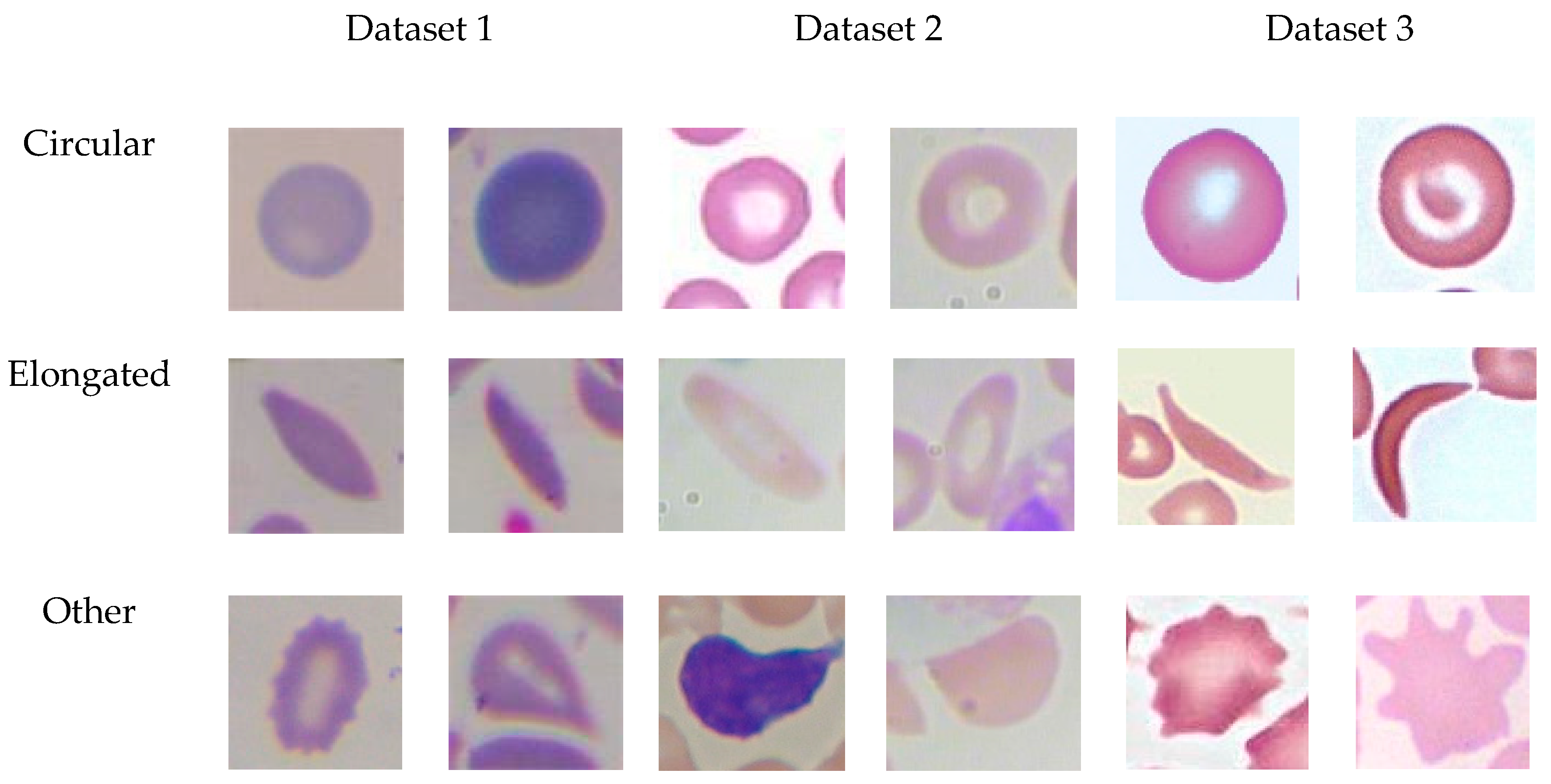
3.1. Datasets
3.1.1. Dataset 1 (Target Dataset)
3.1.2. Dataset2
3.1.3. Dataset3
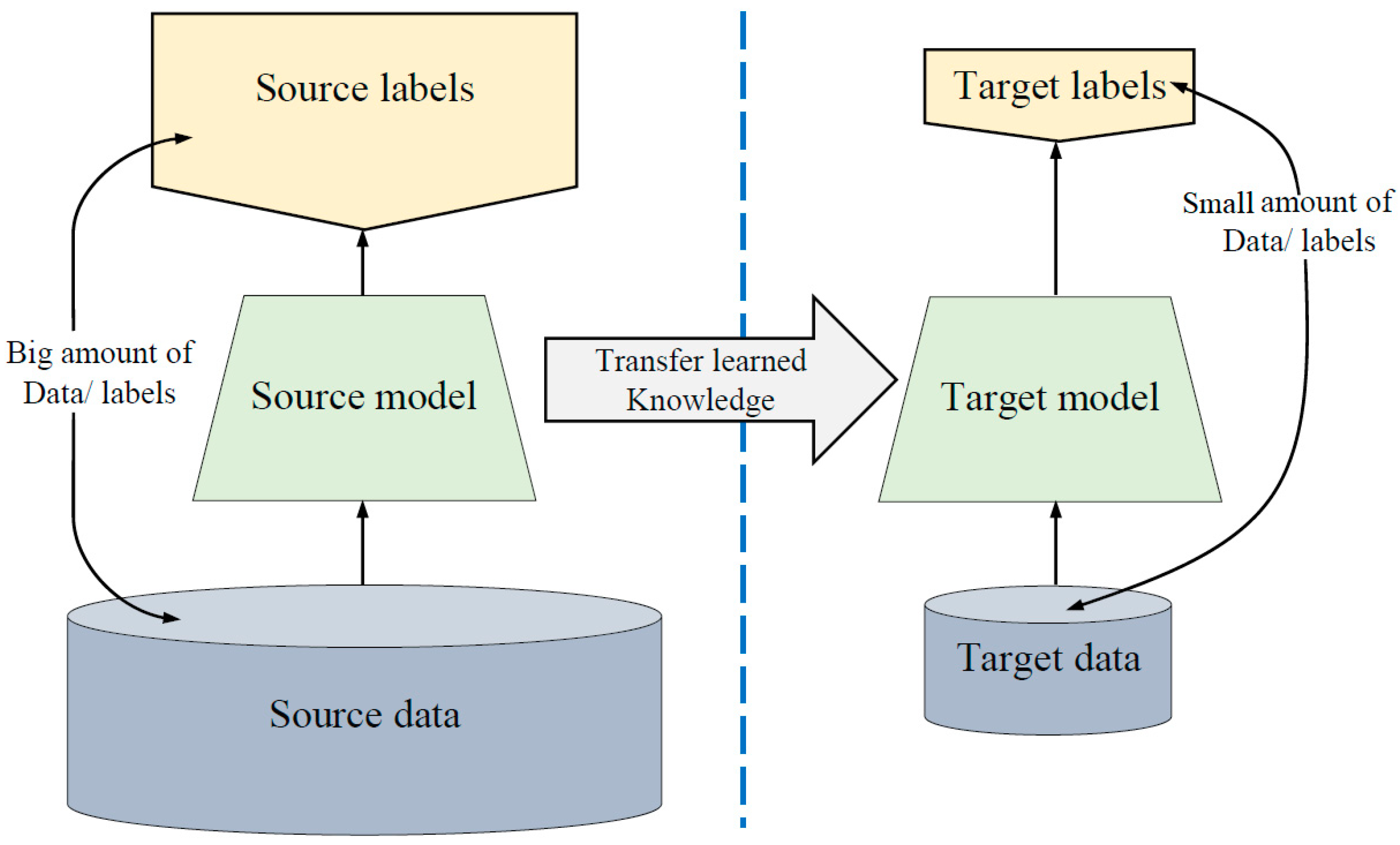
3.2. Lack of Training Data Issue
- Training our proposed models (explained in the next section) on dataset2, which has images that are in the same domain of the target dataset.
- Loading the pre-trained models. The first layers learned low-level features such as colors and edges, while last layers learned task-specific features.
- Replacing the final layers with new layers to learn features specific to the target task.
- Training the fine-tuned models with the target dataset, which is Dataset 1.
- Predicting and evaluating the model accuracy.
- Deploying the results.
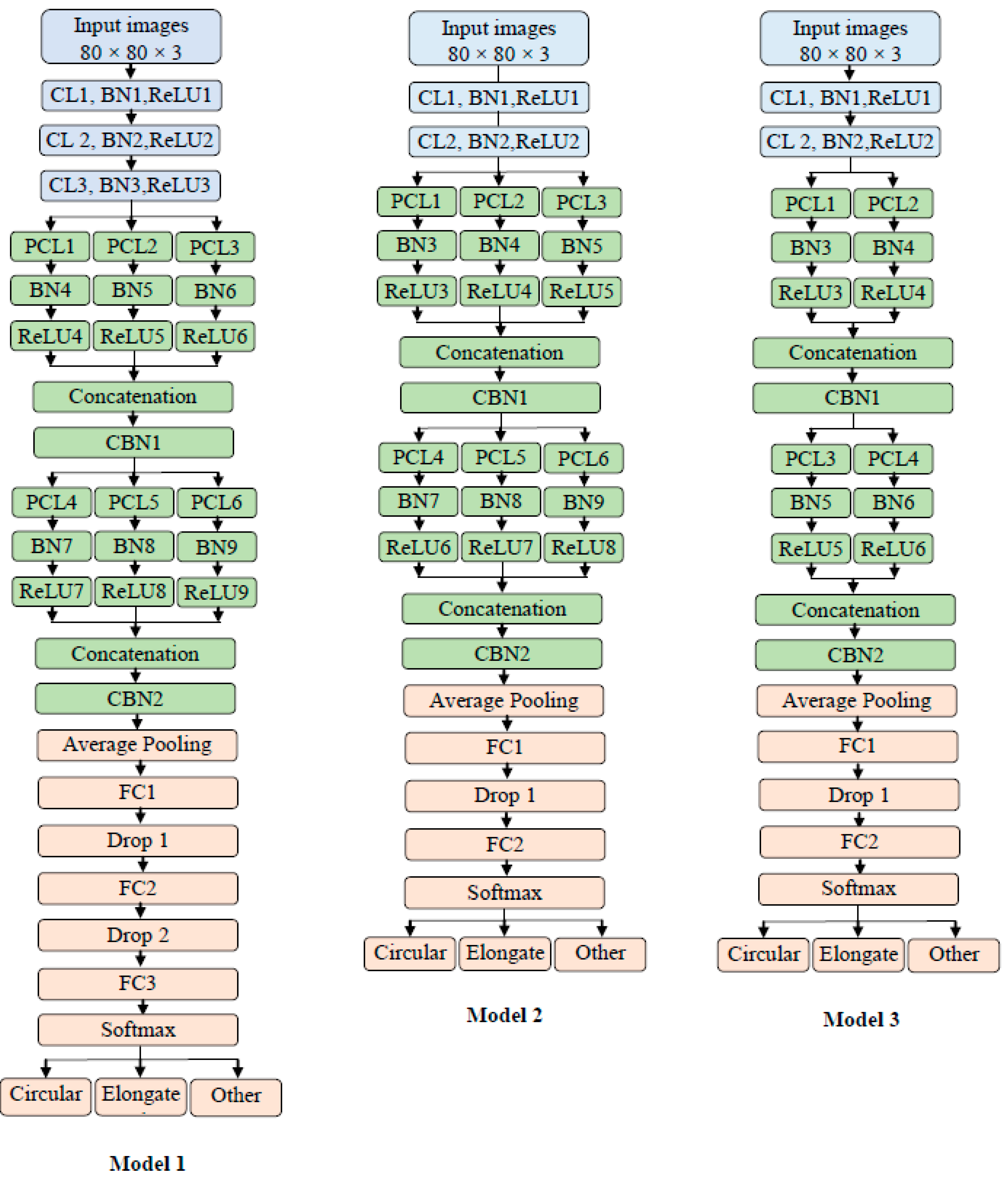
3.3. The Architecture of Proposed Models
3.3.1. Model 1 Architecture
3.3.2. Model 2 Architecture
- Different filters number (the depth)
- Model 2 has two traditional convolutions instead of the three in Model 1
- Model 2 has two fully connected layers and one dropout layer
- The average pooling layer has a filter size of 7 × 7 in Model 2, while in Model 1, the average pooling has a filter size of 4 × 4.
3.3.3. Model 3 Architecture
- Different filter number (the depth)
- Model 3 has two parallel convolutions in both blocks instead of three as in Model 2.
3.4. Training Scenarios
- Scenario 1: Training the models on the original images of the datasets.
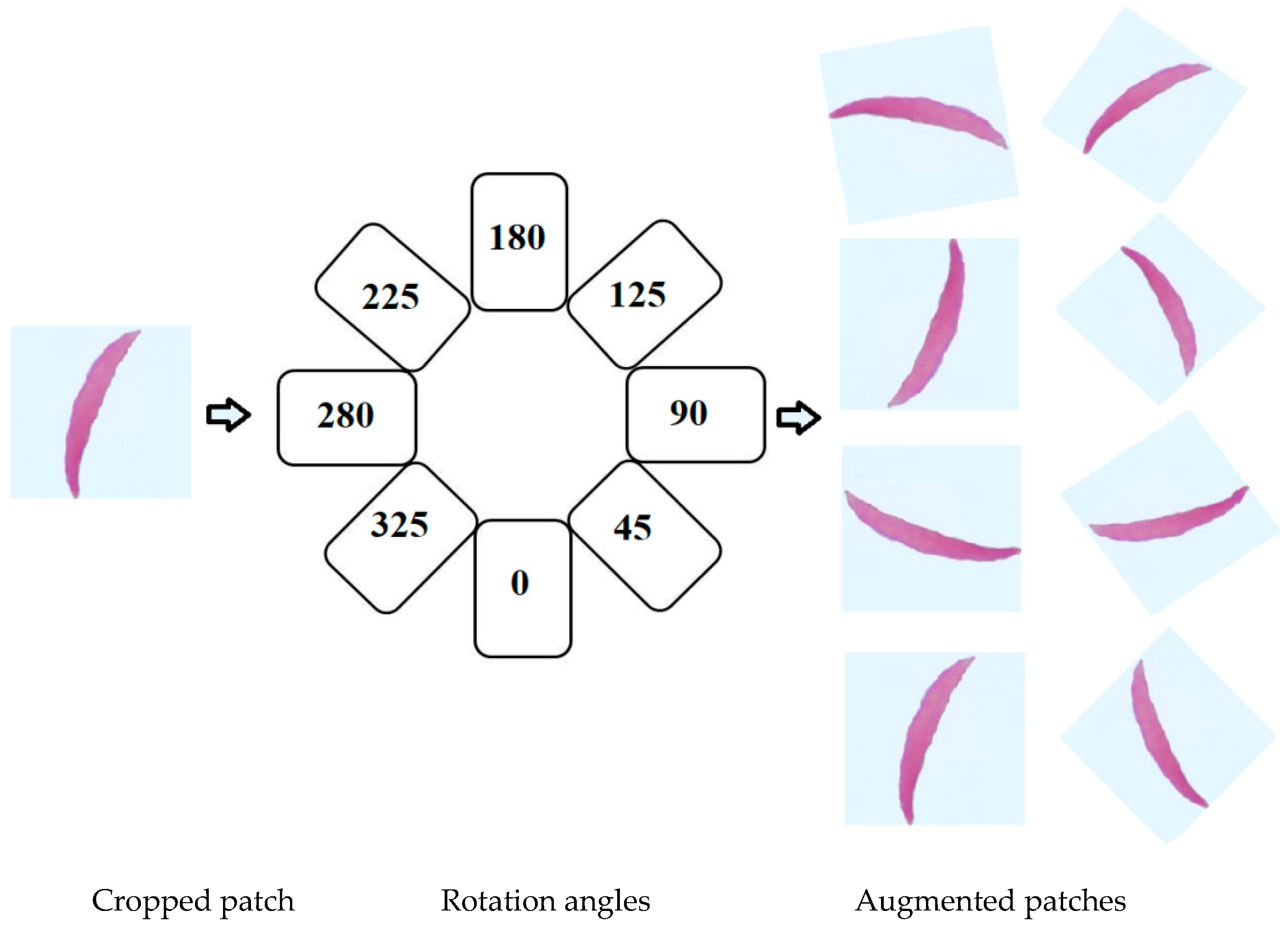
- Scenario 2: Training the models on the original images of the datasets plus augmented images.
- Scenario 3: First, we trained the models on Dataset 2 plus augmented images of Dataset 2 for transfer learning purposes. Then, the models were fine-tuned to train on the original images of the datasets.
- Scenario 4: We repeated Scenario 3 but added in the augmented images with original images.
3.5. Feature Extraction Using Proposed Models
- Loading the data that proposed models tested on for the test phase.
- Loading the trained proposed models to the workspace.
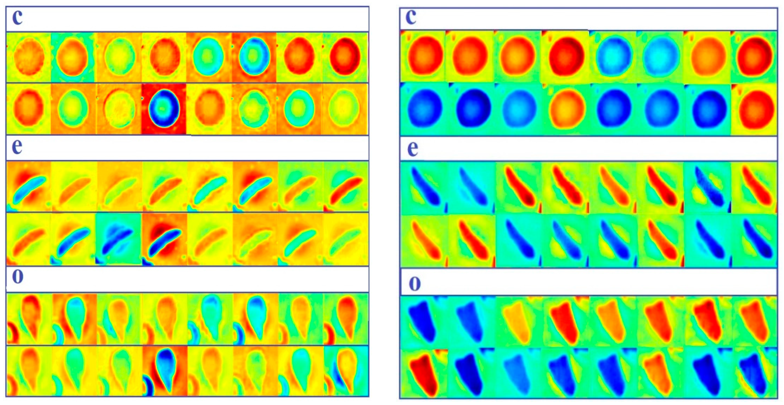
- Extracting the learned features and labels from the last fully connected layer, which represents the last layer before the classifier. The models build a hierarchical representation of input data. Deeper layers hold higher-level features, which were built utilizing the lower-level features of earlier layers. Therefore, we extracted the features from the last fully connected layer.
- Using the extracted features to train a multiclass support vector machine (SVM) classifier. This classifier has been utilized from the Statistics and Machine Learning Toolbox in MATLAB 2019a.
- Classifying the test images using the trained SVM.
- Calculating the accuracy on the test images.
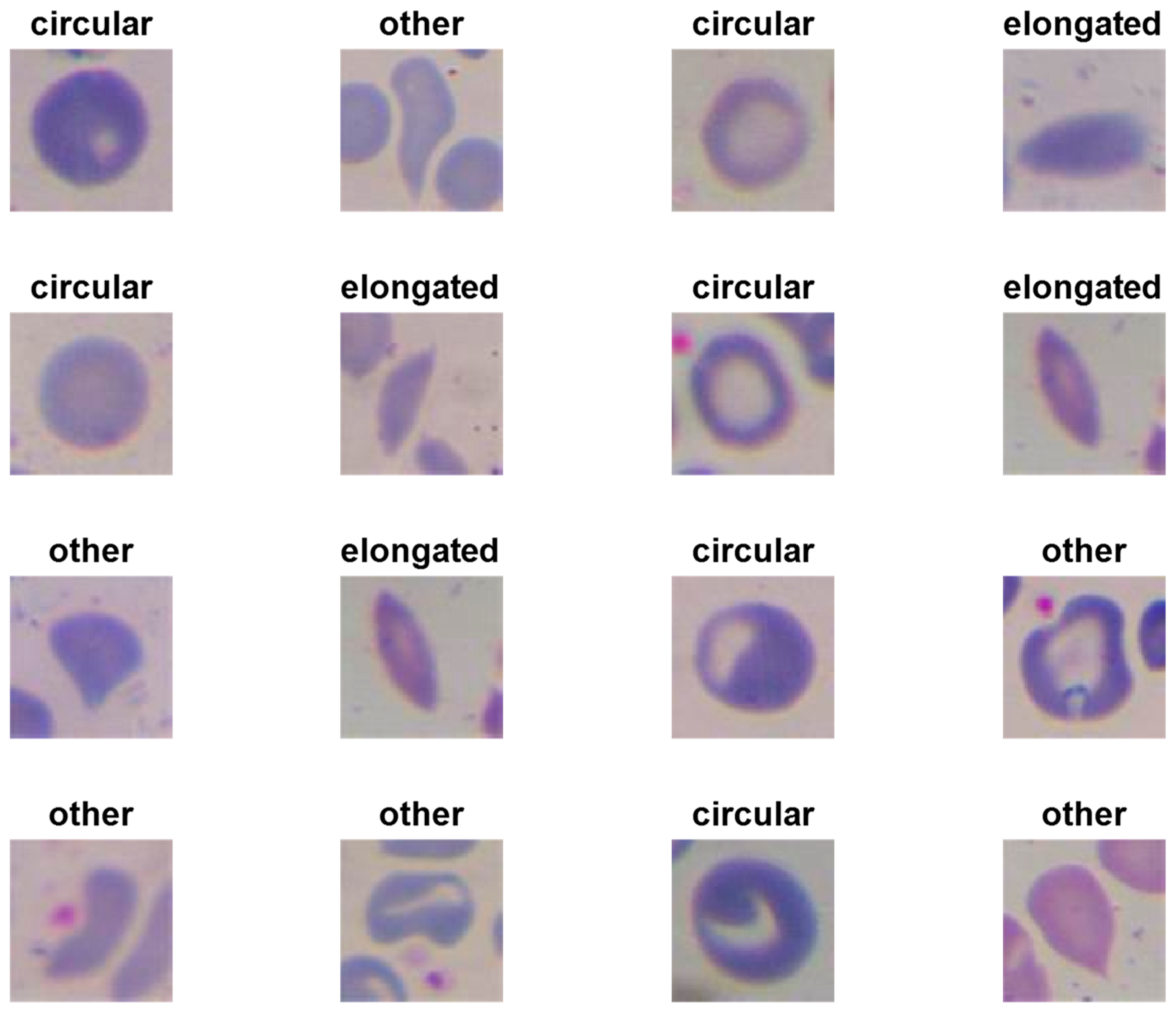
- Plotting some samples of test images with their predicted labels (Figure 6).
4. Experimental Results
- Image augmentation and transfer learning techniques have significantly improved the classification performance of red blood cells classification. Transfer learning from the same domain offers a large benefit to performance.
- Due to using transfer learning from white blood images, our models handled the problem of not paying attention to WBCs in an image, which could lead to a false diagnosis.
- Proposed models are much smaller and shallower than the standard ImageNet models; they performed effectively on two different datasets and handled different cases of overlapped cells.
- Proposed models consumed less training data than other state-of-the-art CNN models such as GoogleNet and ResNet due to the shallow structure of models.
- Overall, all models have achieved high accuracies with Scenarios 3 and 4 compared to prior methods.
- Model 2 has the average number of layers and filters between Model 1 and Model 3, which assisted the model in having sufficient features to differentiate between classes. Model 1 has the largest number of layers and filters compared to Model 2 and Model 3, which requires more big training data; therefore, it achieved the lowest accuracies with Scenarios 1, 2, and 3 of both datasets (1, 3) where there is less training data. It achieved an accuracy that is better than Model 3 when the training set is as big as that in Scenario 4 for both datasets (1, 3). Model 3 has the least number of layers and filters compared to Model 1 and Model 2, which requires a smaller amount of training data; therefore, It achieved higher accuracies with Scenarios 1, 2, and 3 of both datasets (1, 3) than Model 3. While it achieved an accuracy that is less than that of Model 3 when the training set is big as in Scenario 4 of both datasets (1, 3), it requires more layers and filters to differentiate between classes.
- Generally, all proposed models are lightweight models that aided in having a very fast training process besides using GPUs.
- Last but not least, we designed Model 3 first; then, we evaluated its performance. To improve the performance, we increased the width of the model as in Model 2, and it showed good improvement. To improve the performance further, we increased the depth of the network as in Model 1, but that did not improve the performance. Therefore, Model 2 has the best performance.
5. Conclusions
Author Contributions
Funding
Acknowledgments
Conflicts of Interest
References
- Stuart, M.J.; Nagel, R.L. Sickle-cell disease. Lancet 2004, 364, 1343–1360. [Google Scholar] [CrossRef]
- Wąsowicz, M.; Grochowski, M.; Kulka, M.; Mikołajczyk, A.; Ficek, M.; Karpieńko, K.; Cićkiewicz, M. Computed aided system for separation and classification of the abnormal erythrocytes in human blood. In Biophotonics—Riga 2017. Int. Soc. Opt. Photonics 2017, 10592, 105920A. [Google Scholar]
- Alzubaidi, L.; Fadhel, M.A.; Al-Shamma, O.; Zhang, J. Robust and Efficient Approach to Diagnose Sickle Cell Anemia in Blood. In International Conference on Intelligent Systems Design and Applications; Springer: Cham, Switzerland, December 2018; pp. 560–570. [Google Scholar]
- Survey Data. Available online: https://www.cdc.gov/ncbddd/sicklecell/data.html (accessed on 25 December 2019).
- Acharya, V.; Prakasha, K. Computer-Aided Technique to Separate the Red Blood Cells, Categorize them and Diagnose Sickle Cell Anemia. J. Eng. Sci. Technol. Rev. 2019, 12, 2. [Google Scholar] [CrossRef]
- Das, P.K.; Meher, S.; Panda, R.; Abraham, A. A Review of Automated Methods for the Detection of Sickle Cell Disease. IEEE Rev. Biomed. Eng. 2019, 13, 309–324. [Google Scholar] [CrossRef] [PubMed]
- Huang, Z.; Lin, J.; Xu, L.; Wang, H.; Bai, T.; Pang, Y.; Meen, T.-H. Fusion High-Resolution Network for Diagnosing ChestX-ray Images. Electronics 2020, 9, 190. [Google Scholar] [CrossRef]
- Nurmaini, S.; Darmawahyuni, A.; Sakti Mukti, A.N.; Rachmatullah, M.N.; Firdaus, F.; Tutuko, B. Deep Learning-Based Stacked Denoising and Autoencoder for ECG Heartbeat Classification. Electronics 2020, 9, 135. [Google Scholar] [CrossRef]
- Alzubaidi, L.; Fadhel, M.A.; Oleiwi, S.R.; Al-Shamma, O.; Zhang, J. DFU_QUTNet: Diabetic foot ulcer classification using novel deep convolutional neural network. Multimed. Tools Appl. 2019, 1–23. [Google Scholar] [CrossRef]
- LeCun, Y.; Bengio, Y.; Hinton, G. Deep learning. Nature 2015, 521, 436. [Google Scholar] [CrossRef]
- Patil, P.R.; Sable, G.S.; Anandgaonkar, G. Counting of WBCs and RBCs from blood images using gray thresholding. Int. J. Res. Eng. Technol. 2014, 3, 391–395. [Google Scholar]
- Alomari, Y.M.; Abdullah, S.; Huda, S.N.; Zaharatul Azma, R.; Omar, K. Automatic detection and quantification of WBCs and RBCs using iterative structured circle detection algorithm. Comput. Math. Methods Med. 2014, 2014, 979302. [Google Scholar] [CrossRef]
- Bhagavathi, S.L.; Niba, S.T. An automatic system for detecting and counting RBC and WBC using fuzzy logic. Arpn J. Eng. Appl. Sci. 2016, 11, 6891–6894. [Google Scholar]
- Maitra, M.; Gupta, R.K.; Mukherjee, M. Detection and counting of red blood cells in blood cell images using Hough transform. Int. J. Comput. Appl. 2012, 53, 16. [Google Scholar] [CrossRef]
- Thejashwini, M.; Padma, M.C. Counting of RBC’s and WBC’s Using Image Processing Technique. Int. J. Recent Innov. Trends Comput. Commun. 2015, 3, 2948–2953. [Google Scholar]
- Mazalan, S.M.; Mahmood, N.H.; Razak, M.A.A. Automated red blood cells counting in peripheral blood smear image using circular Hough transform. In Proceedings of the 2013 1st IEEE International Conference on Artificial Intelligence, Modelling and Simulation, Kota Kinabalu, Malaysia, 3–5 December 2013; pp. 320–324. [Google Scholar]
- Tulsani, H.; Saxena, S.; Yadav, N. Segmentation using morphological watershed transformation for counting blood cells. IJCAIT 2013, 2, 28–36. [Google Scholar]
- Sreekumar, A.; Bhattacharya, A. Identification of sickle cells from microscopic blood smear image using image processing. Int. J. Emerg. Trends Sci. Technol. 2014, 1, 783–787. [Google Scholar]
- Chintawar, I.A.; Aishvarya, M.; Kuhikar, C. Detection of sickle cells using image processing. Int. J. Sci. Technol. Eng. 2016, 2, 335–339. [Google Scholar]
- Patil, D.N.; Khot, U.P. Image processing based abnormal blood cells detection. Int. J. Tech. Res. Appl. 2015, 31, 37–43. [Google Scholar]
- Sahu, M.; Biswas, A.K.; Uma, K. Detection of Sickle Cell Anemia in Red Blood Cell. Int. J. Eng. Appl. Sci. (Ijeas) 2015, 2, 3. [Google Scholar]
- Rexcy, S.M.A.; Akshaya, V.S.; Swetha, K.S. Effective use of image processing techniques for the detection of sickle cell anemia and presence of plasmodium parasites. Int. J. Adv. Res. Innov. Ideas Educ. 2016, 2, 701–706. [Google Scholar]
- Rakshit, P.; Bhowmik, K. Detection of abnormal findings in human RBC in diagnosing sickle cell anaemia using image processing. Procedia Technol. 2013, 10, 28–36. [Google Scholar] [CrossRef]
- Revathi, T.; Jeevitha, S. Efficient watershed based red blood cell segmentation from digit al images in sickle cell disease. Int. J. Sci. Eng. Appl. Sci. 2016, 2, 300–317. [Google Scholar]
- Bala, S.; Doegar, A. Automatic detection of sickle cell in red blood cell using watershed segmentation. Int. J. Adv. Res. Comput. Commun. Eng. 2015, 4, 488–491. [Google Scholar]
- Gonzalez-Hidalgo, M.; Guerrero-Pena, F.A.; Herold-Garcia, S.; Jaume-i-Capó, A.; Marrero-Fernández, P.D. Red blood cell cluster separation from digital images for use in sickle cell disease. IEEE J. Biomed. Health Inform. 2014, 19, 1514–1525. [Google Scholar] [CrossRef] [PubMed]
- Parvathy, H.B.; Hariharan, S.; Aruna, S.N. A Real Time System for the Analysis of Sickle Cell Anemia Blood Smear Images Using Image Processing. Int. J. Innov. Res. Sci. Eng. Technol. 2016, 5, 6200–6207. [Google Scholar]
- Veluchamy, M.; Perumal, K.; Ponuchamy, T. Feature extraction and classification of blood cells using artificial neural network. Am. J. Appl. Sci. 2012, 9, 615. [Google Scholar]
- Poomcokrak, J.; Neatpisarnvanit, C. Red blood cells extraction and counting. In Proceedings of the 3rd International Symposium on Biomedical Engineering, Changsha, China, 8–10 June 2008; pp. 199–203. [Google Scholar]
- AbdulraheemFadhel, M.; Humaidi, A.J.; RazzaqOleiwi, S. Image processing-based diagnosis of sickle cell anemia in erythrocytes. In Proceedings of the 2017 Annual Conference on New Trends in Information & Communications Technology Applications (NTICT) IEEE, Baghdad, Iraq, 7–9 March 2017; pp. 203–207. [Google Scholar]
- Sharma, V.; Rathore, A.; Vyas, G. Detection of sickle cell anaemia and thalassaemia causing abnormalities in thin smear of human blood sample using image processing. In Proceedings of the 2016 International Conference on Inventive Computation Technologies (ICICT), Coimbatore, India, 26–27 August 2016; pp. 1–5. [Google Scholar]
- Rodrigues, L.F.; Naldi, M.C.; Mari, J.F. Morphological analysis and classification of erythrocytes in microscopy images. In Proceedings of the 2016 Workshop de Visão Computacional, Campo Grande, Brazil, 9–11 November 2016; pp. 1–6. [Google Scholar]
- Chen, H.M.; Tsao, Y.T.; Tsai, S.N. Automatic image segmentation and classification based on direction texton technique for hemolytic anemia in thin blood smears. Mach. Vis. Appl. 2014, 25, 501–510. [Google Scholar] [CrossRef]
- Acharya, V.; Kumar, P. Identification and red blood cell classification using computer aided system to diagnose blood disorders. In Proceedings of the 2017 IEEE International Conference on Advances in Computing, Communications and Informatics (ICACCI), Udupi, India, 13–16 September 2017; pp. 2098–2104. [Google Scholar]
- Elsalamony, H.A. Anaemia cells detection based on shape signature using neural networks. Measurement 2017, 104, 50–59. [Google Scholar] [CrossRef]
- Albayrak, B.; Darici, M.B.; Kiraci, F.; Öğrenci, A.S.; Özmen, A.; Ertez, K. Orak Hücreli Anemi Tespiti Sickle Cell Anemia Detection. In Proceedings of the 2018 IEEE Medical Technologies National Congress (TIPTEKNO), Magusa, Cyprus, 8–10 November 2018; pp. 1–4. [Google Scholar]
- Chy, T.S.; Rahaman, M.A. Automatic Sickle Cell Anemia Detection Using Image Processing Technique. In Proceedings of the 2018 IEEE International Conference on Advancement in Electrical and Electronic Engineering (ICAEEE), Gazipur, Bangladesh, 22–24 November 2018; pp. 1–4. [Google Scholar]
- Chy, T.S.; Rahaman, M.A. A Comparative Analysis by KNN, SVM & ELM Classification to Detect Sickle Cell Anemia. In Proceedings of the 2019 IEEE International Conference on Robotics, Electrical and Signal Processing Techniques (ICREST), Dhaka, Bangladesh, 10–12 January 2019; pp. 455–459. [Google Scholar]
- Alzubaidi, L.; Al-Shamma, O.; Fadhel, M.A.; Farhan, L.; Zhang, J. Classification of Red Blood Cells in Sickle Cell Anemia Using Deep Convolutional Neural Network. In International Conference on Intelligent Systems Design and Applications; Springe: Cham, Switzerland, 2018; pp. 550–559. [Google Scholar]
- Xu, M.; Papageorgiou, D.P.; Abidi, S.Z.; Dao, M.; Zhao, H.; Karniadakis, G.E. A deep convolutional neural network for classification of red blood cells in sickle cell anemia. PLoS Comput. Biol. 2017, 13, e1005746. [Google Scholar] [CrossRef]
- Parthasarathy, D. WBC-Classification. Available online: https://github.com/dhruvp/wbc-classification/tree/master/Original_Images (accessed on 15 November 2019).
- Wadsworth-Center. White Blood Cell Images. Available online: https://www.wadsworth.org/ (accessed on 10 November 2019).
- Al-Dulaimi, K.; Chandran, V.; Banks, J.; Tomeo-Reyes, I.; Nguyen, K. Classification of white blood cells using bispectral invariant features of nuclei shape. In Proceedings of the 2018 IEEE Digital Image Computing: Techniques and Applications (DICTA), Canberra, Australia, 10–13 December 2018; pp. 1–8. [Google Scholar]
- Labati, R.D.; Piuri, V.; Scotti, F. All-IDB: The acute lymphoblastic leukemia image database for image processing. In Proceedings of the 2011 18th IEEE International Conference on Image Processing, Brussels, Belgium, 11–14 September 2011; pp. 2045–2048. [Google Scholar]
- Sickle Cells Anemia. Available online: http://sicklecellanaemia.org/ (accessed on 1 September 2019).
- Fang, B.; Lu, Y.; Zhou, Z.; Li, Z.; Yan, Y.; Yang, L.; Jiao, G.; Li, G. Classification of Genetically Identical Left and Right Irises Using a Convolutional Neural Network. Electronics 2019, 8, 1109. [Google Scholar] [CrossRef]
- Lee, H.; Lee, J. A Deep Learning-Based Scatter Correction of Simulated X-ray Images. Electronics 2019, 8, 944. [Google Scholar] [CrossRef]
- Li, Y.; Richtarik, P.; Ding, L.; Gao, X. On the decision boundary of deep neural networks. arXiv 2018, arXiv:abs/1808.05385. Available online: https://arxiv.org/abs/1808.05385 (accessed on 9 December 2019).
- Kermany, D.S.; Goldbaum, M.; Cai, W.; Valentim, C.C.; Liang, H.; Baxter, S.L.; Dong, J. Identifying medical diagnoses and treatable diseases by image-based deep learning. Cell 2018, 172, 1122–1131. [Google Scholar] [CrossRef] [PubMed]
- Yosinski, J.; Clune, J.; Bengio, Y.; Lipson, H. How transferable are features in deep neural networks? In Proceedings of the Neural Information Processing Systems 2014, Montreal, QC, Canada, 8–13 December 2014; pp. 3320–3328. [Google Scholar]
- Pan, S.J.; Yang, Q. A survey on transfer learning. IEEE Trans. Knowl. Data Eng. 2009, 22, 1345–1359. [Google Scholar] [CrossRef]
- Deng, J.; Dong, W.; Socher, R.; Li, L.J.; Li, K.; Fei-Fei, L. ImageNet: A large-scale hierarchical image database. In Proceedings of the 2009 IEEE conference on computer vision and pattern recognition, Miami, FL, USA, 20–25 June 2009; pp. 248–255. [Google Scholar]
- Cook, D.; Feuz, K.D.; Krishnan, N.C. Transfer learning for activity recognition: A survey. Knowl. Inf. Syst. 2013, 36, 537–556. [Google Scholar] [CrossRef]
- Cao, X.; Wang, Z.; Yan, P.; Li, X. Transfer learning for pedestrian detection. Neurocomputing 2013, 100, 51–57. [Google Scholar] [CrossRef]
- Raghu, M.; Zhang, C.; Kleinberg, J.; Bengio, S. Transfusion: Understanding transfer learning for medical imaging. In Proceedings of the Neural Information Processing Systems 2019, Vancouver, BC, Canada, 8–14 December 2019; pp. 3342–3352. [Google Scholar]
- Tan, C.; Sun, F.; Kong, T.; Zhang, W.; Yang, C.; Liu, C. A survey on deep transfer learning. In International Conference on Artificial Neural Networks; Springer: Cham, Switzerland, October 2018; pp. 270–279. [Google Scholar]
- Van Dyk, D.A.; Meng, X.L. The art of data augmentation. J. Comput. Graph. Stat. 2001, 10, 1–50. [Google Scholar] [CrossRef]
- Lv, E.; Wang, X.; Cheng, Y.; Yu, Q. Deep ensemble network based on multi-path fusion. Artif. Intell. Rev. 2019, 52, 151–168. [Google Scholar] [CrossRef]
- Lv, E.; Wang, X.; Cheng, Y.; Yu, Q. Deep convolutional network based on pyramid architecture. IEEE Access 2018, 6, 43125–43135. [Google Scholar] [CrossRef]
- Wang, J.; Wei, Z.; Zhang, T.; Zeng, W. Deeply-fused nets. arXiv 2016, arXiv:Abs/1605.07716. [Google Scholar]
- Simonyan, K.; Zisserman, A. Very deep convolutional networks for large-scale image recognition. arXiv 2014, arXiv:Abs/1409.1556. Available online: https://arxiv.org/abs/1409.1556 (accessed on 9 December 2019).
- Krizhevsky, A.; Sutskever, I.; Hinton, G.E. ImageNet classification with deep convolutional neural networks. In Proceedings of the Neural Information Processing Systems 2012, Lake Tahoe, NV, USA, 3–6 December 2012; pp. 1097–1105. [Google Scholar]
- He, K.; Zhang, X.; Ren, S.; Sun, J. Deep residual learning for image recognition. In Proceedings of the IEEE conference on computer vision and pattern recognition, Las Vegas, NV, USA, 27–30 June 2016; pp. 770–778. [Google Scholar]
- Srivastava, N.; Hinton, G.; Krizhevsky, A.; Sutskever, I.; Salakhutdinov, R. Dropout: A simple way to prevent neural networks from overfitting. J. Mach. Learn. Res. 2014, 15, 1929–1958. [Google Scholar]
- Gual-Arnau, X.; Herold-García, S.; Simó, A. Erythrocyte shape classification using integral-geometry-based methods. Med. Biol. Eng. Comput. 2015, 53, 623–633. [Google Scholar] [CrossRef] [PubMed]
- De Faria, L.C.; Rodrigues, L.F.; Mari, J.F. Cell classification using handcrafted features and bag of visual words. In Proceedings of the Workshop de Visão Computacional, Ilhéus-BA, Brazil, 12–14 November 2018. [Google Scholar]


| Name of Layer | Filter Size (FS) and Stride (S) | Activations |
|---|---|---|
| Input layer | - | 80 × 80 × 3 |
| CL 1, BN 1, ReLU 1 | FS = 1 × 1, S = 1 | 80 × 80 × 64 |
| CL 2, BN 2, ReLU 2 | FS = 3 × 3, S = 2 | 40 × 40 × 64 |
| CL 3, BN 3, ReLU 3 | FS = 5 × 5, S = 2 | 20 × 20 × 64 |
| PCL 1, BN 4, ReLU 4 | FS = 1 × 1, S = 1 | 20 × 20 × 128 |
| PCL 2, BN 5, ReLU 5 | FS = 3 × 3, S = 1 | 20 × 20 × 128 |
| PCL 3, BN 6, ReLU 6 | FS = 5 × 5, S = 1 | 20 × 20 × 128 |
| Concatenation Layer 1 | Three inputs | 20 × 20 × 384 |
| CBN 1 | Batch Normalization | 20 × 20 × 384 |
| PCL 4, BN 7, ReLU 7 | FS = 1 × 1, S = 2 | 10 × 10 × 256 |
| PCL 5, BN 8, ReLU 8 | FS = 3 × 3, S = 2 | 10 × 10 × 256 |
| PCL 6, BN 9, ReLU 9 | FS = 5 × 5, S = 2 | 10 × 10 × 256 |
| Concatenation Layer 2 | Three inputs | 10 × 10 × 768 |
| CBN 2 | Batch Normalization | 10 × 10 × 768 |
| Average Pooling | Size = 4 × 4, S = 2 | 4 × 4 × 768 |
| FC1 | 600 | 1 × 1 × 600 |
| Drop 1 | Learning rate: 0.5 | 1 × 1 × 600 |
| FC 2 | 150 | 1 × 1 × 150 |
| Drop 2 | Learning rate: 0.5 | 1 × 1 × 150 |
| FC 3 | 3 | 1 × 1 × 3 |
| Softmax and Classoutput | 3 classes: circular, elongated, other | - |
| Name of Layer | Filter Size (FS) and Stride (S) | Activations |
|---|---|---|
| Input layer | - | 80 × 80 × 3 |
| CL 1, BN 1, ReLU 1 | FS = 3 × 3, S = 1 | 80 × 80 × 16 |
| CL 2, BN 2, ReLU 2 | FS = 5 × 5, S = 2 | 40 × 40 × 16 |
| PCL 1, BN 3, ReLU 3 | FS = 1 × 1, S = 1 | 40 × 40 × 32 |
| PCL 2, BN 4, ReLU 4 | FS = 3 × 3, S = 1 | 40 × 40 × 32 |
| PCL 3, BN 5, ReLU 5 | FS = 5 × 5, S = 1 | 40 × 40 × 32 |
| Concatenation Layer 1 | Three inputs | 40 × 40 × 96 |
| CBN 1 | Batch Normalization | 40 × 40 × 96 |
| PCL 4, BN 6, ReLU 6 | FS = 1 × 1, S = 2 | 20 × 20 × 64 |
| PCL 5, BN 7, ReLU 7 | FS = 3 × 3, S = 2 | 20 × 20 × 64 |
| PCL 6, BN 8, ReLU 8 | FS = 5 × 5, S = 2 | 20 × 20 × 64 |
| Concatenation Layer 2 | Three inputs | 20 × 20 × 192 |
| CBN 2 | Batch Normalization | 20 × 20 × 192 |
| Average Pooling | Size = 7 × 7, S = 2 | 7 × 7 × 192 |
| FC 1 | 90 | 1 × 1 × 90 |
| Drop 1 | learning rate:0.5 | 1 × 1 × 90 |
| FC 2 | 3 | 1 × 1 × 3 |
| Softmax and Classoutput | 3 classes: circular, elongated, other | - |
| Name of Layer | Filter Size (FS) and Stride (S) | Activations |
|---|---|---|
| Input layer | - | 80 × 80 × 3 |
| CL 1, BN 1, ReLU 1 | FS = 3 × 3, S = 1 | 80 × 80 × 16 |
| CL 2, BN 2, ReLU 2 | FS = 5 × 5, S = 2 | 40 × 40 × 16 |
| PCL 1, BN 3, ReLU 3 | FS = 1 × 1, S = 1 | 40 × 40 × 16 |
| PCL 2, BN 4, ReLU 4 | FS = 3 × 3, S = 1 | 40 × 40 × 16 |
| Concatenation Layer 1 | Three inputs | 40 × 40 × 32 |
| CBN 1 | Batch Normalization | 40 × 40 × 32 |
| PCL 3, BN 5, ReLU 5 | FS = 1 × 1, S = 2 | 20 × 20 × 32 |
| PCL 4, BN 6, ReLU 6 | FS = 3 × 3, S = 2 | 20 × 20 × 32 |
| Concatenation Layer 2 | Three inputs | 20 × 20 × 64 |
| CBN 2 | Batch Normalization | 20 × 20 × 64 |
| Average Pooling | Size = 7 × 7, S = 2 | 7 × 7 × 64 |
| FC 1 | 60 | 1 × 1 × 60 |
| Drop 1 | Learning rate: 0.5 | 1 × 1 × 60 |
| FC 2 | 3 | 1 × 1 × 3 |
| Softmax and Classoutput | 3 classes: circular, elongated, other | 1 × 1 × 3 |
| Scenarios | Model 1 (%) | Model 2 (%) | Model 3 (%) | |
|---|---|---|---|---|
| Dataset 1 (erythrocytesIDB1) | Scenario 1 | 85.40 | 88.60 | 86.17 |
| Scenario 2 | 91.21 | 93.87 | 92.34 | |
| Scenario 3 | 97.43 | 98.40 | 98.06 | |
| Scenario 4 | 98.57 | 99.54 | 98.31 | |
| Dataset 3 | Scenario 1 | 82.63 | 83.99 | 83.50 |
| Scenario 2 | 90.11 | 92.01 | 91.12 | |
| Scenario 3 | 95.65 | 97.17 | 96.55 | |
| Scenario 4 | 97.66 | 98.87 | 97.61 |
| Scenarios | Model 1 (%) | Model 2 (%) | Model 3 (%) |
|---|---|---|---|
| Scenario1 | 87.10 | 90.80 | 89.88 |
| Scenario2 | 92.27 | 94.87 | 92.79 |
| Scenario3 | 97.09 | 98.10 | 97.16 |
| Scenario4 | 99.57 | 99.98 | 99.44 |
| Method | Accuracy (%) |
|---|---|
| Gual-Arnau et al. 2015 [65] | 96.10 |
| Rodrigues et al. 2016 [32] | 93.18 |
| Rodrigues et al. 2016 [32] | 93.07 |
| Rodrigues et al. 2016 [32] | 94.59 |
| de Faria et al. 2018 [66] | 92.52 |
| de Faria et al. 2018 [66] | 93.67 |
| Our method (Scenario 4, Model 2) | 99.54 |
| Our method (Scenario 4, Model2 +SVM) | 99.98 |
© 2020 by the authors. Licensee MDPI, Basel, Switzerland. This article is an open access article distributed under the terms and conditions of the Creative Commons Attribution (CC BY) license (http://creativecommons.org/licenses/by/4.0/).
Share and Cite
Alzubaidi, L.; Fadhel, M.A.; Al-Shamma, O.; Zhang, J.; Duan, Y. Deep Learning Models for Classification of Red Blood Cells in Microscopy Images to Aid in Sickle Cell Anemia Diagnosis. Electronics 2020, 9, 427. https://doi.org/10.3390/electronics9030427
Alzubaidi L, Fadhel MA, Al-Shamma O, Zhang J, Duan Y. Deep Learning Models for Classification of Red Blood Cells in Microscopy Images to Aid in Sickle Cell Anemia Diagnosis. Electronics. 2020; 9(3):427. https://doi.org/10.3390/electronics9030427
Chicago/Turabian StyleAlzubaidi, Laith, Mohammed A. Fadhel, Omran Al-Shamma, Jinglan Zhang, and Ye Duan. 2020. "Deep Learning Models for Classification of Red Blood Cells in Microscopy Images to Aid in Sickle Cell Anemia Diagnosis" Electronics 9, no. 3: 427. https://doi.org/10.3390/electronics9030427
APA StyleAlzubaidi, L., Fadhel, M. A., Al-Shamma, O., Zhang, J., & Duan, Y. (2020). Deep Learning Models for Classification of Red Blood Cells in Microscopy Images to Aid in Sickle Cell Anemia Diagnosis. Electronics, 9(3), 427. https://doi.org/10.3390/electronics9030427