Abstract
Linear prediction is the kernel technology in speech processing. It has been widely applied in speech recognition, synthesis, and coding, and can efficiently and correctly represent the speech frequency spectrum with only a few parameters. Line Spectrum Pairs (LSPs) frequencies, as an alternative representation of Linear Predictive Coding (LPC), have the advantages of good quantization accuracy and low spectral sensitivity. However, computing the LSPs frequencies takes a long time. To address this issue, a fast computation algorithm, based on the Bairstow method for computing LSPs frequencies from linear prediction coefficients, is proposed in this paper. The algorithm process first transforms the symmetric and antisymmetric polynomial to general polynomial, then extracts the polynomial roots. Associated with the short-term stationary property of speech signal, an adaptive initial method is applied to reduce the average iteration numbers by 26%, as compared to the statics in the initial method, with a Perceptual Evaluation of Speech Quality (PESQ) score reaching 3.46. Experimental results show that the proposed method can extract the polynomial roots efficiently and accurately with significantly reduced computation complexity. Compared to previous works, the proposed method is 17 times faster than Tschirnhus Transform, and has a 22% PESQ improvement on the Birge-Vieta method with an almost comparable computation time.
1. Introduction
Linear predictive analysis of the speech signal is one of the most powerful speech analysis techniques, which can extract the short-time spectral envelope information of speech signals efficiently, and is widely used in the fields of speech representing for low bit rate transmission or storage, automatic speech and speaker recognition [1,2,3,4,5]. The predominant linear predictive analysis method is Linear Prediction Coding (LPC), featuring better fault tolerance during transmitting spectral envelope information. As an alternative representation of LPC, Line Spectrum Pairs (LSPs) were first introduced by Itakura [6], which have the advantages of good quantization accuracy and low spectral sensitivity.
During the computation of LSPs, the LPC polynomial A(z) is decomposed into a pair of symmetric and anti-symmetric polynomials. These two polynomials are called LPC polynomials. It has been proven that the roots of the LPC polynomials, namely the LSPs frequencies, are interleaved on the unit circle [6]. Many methods have been proposed to solve these LPC polynomials. Soong and Juang [7,8] adopted the Discrete Cosine Transform (DCT) to evaluate the cosine functions, based on the bisection method with a fine grid. They employed a closed formula to extract the roots of LPC polynomial. Kang and Fransen [9] first proposed to transform the LPC polynomial into the sum of cosine functions to avoid the complex computation in later processing. They employed the autocorrelation method and the all-pass filter to extract the roots. Despite these methods solving the LPC polynomials correctly, they have the disadvantages of high computational complexity from trigonometric functions, and high memory usage from cosine tables. Kabal and Ramachandram [10] employed the bisection method and the interpolation property to locate the position of zero-crossings with a fine grid. While it requires no prior storages or the calculation of trigonometric functions, the number of bisections cannot be decreased without compromising the search of zero-crossings. Wu and Chen [11] first proposed to transform LPC polynomial into a pair of general-form polynomials, then used the closed-form formulas and the modified Newton-Raphson method to extract polynomial roots. It can avoid the computation of trigonometric functions with a fine grid. However, the mathematical operations with complex numbers are still time-consuming. Chen and Ruan [12] proposed the modified complex-free Ferrari formula to reduce the computation. While this algorithm avoids complex number operations, it still needs modulus operations to get the roots of the polynomials. Chen and Chang [13] employed the Tschirnhaus transform to reduce the degree of the polynomials, then used Descartes–Euler to extract the roots. While it can accelerate the computation processing, it still needs to compute trigonometric functions. Chung-Hsien Chang [14] proposed a method to solve the LPC polynomials, which is suitable for hardware implementation.
Hence, an efficient method to solve LPC polynomials should have the following characteristics:
- Avoiding evaluation of trigonometric functions,
- Avoiding using complex operations and a fine grid,
- Extracting the roots rapidly and accurately.
Considering the above requirements, we proposed a fast LPC computation method, based on the Bairstow method, which can extract the roots of LPC polynomials without using complex operations, a fine grid and trigonometric functions. Luk [15] and Hsiao [16] used the Bairstow method to solve the polynomial, but without specific algorithm implementation and performance evaluation of the algorithm. Additionally, the initial method was stubborn, which limited the convergence speed. Thus, an adaptive initial method, associated with the short-term property of the speech signal, is proposed to guarantee its convergence in this paper. Then, we apply our method to a speech compression codec system. Experiments show that, compared with other methods, including those of Soong and Juang [8], Kabal and Ramachandram [10], the Chen and Wu method [11], the modified Ferrari’s formula [12], Tschirnhaus transform [13], the Birge-Vieta method [14] and the previous Braistow-base LPC analysis methods [15,16], the proposed method can estimate the LSPs frequencies accurately with the lowest computational complexity, together with high speech quality.
The rest of this paper is organized as follows: A brief introduction of LSPs frequencies is reviewed in Section 2. In Section 3, a detail description of the Bairstow method is given, then the adaptive initial method is given to boost the estimation accuracy and the convergence speed. Section 4 provides a guideline to estimate the 10-order LSPs, and shows the experimental results of the proposed method, as compared to previous methods. Finally, Section 5 provides the conclusion.
2. Line Spectral Pairs (LSPs) Frequencies
2.1. LPC Polynomial
This section introduces the background of the LSPs frequencies and some of the relevant properties briefly. Given a p-order LPC, the minimum-phase LPC polynomial is expressed as follows, according to Reference [14]:
where ,, …, are the direct form of LPC coefficients. The LPC polynomial can be decomposed into a symmetric polynomial and an anti-symmetric polynomial. The following formulas are their representations:
The roots of and determine the value of LSPs frequencies. According to Reference [14], the above two auxiliary polynomials have the significant properties that their roots are on the unit circle and interleave with each other. Further, has a root , and has a root . These roots can be eliminated by polynomial division. Thus, the reduced polynomials can be obtained
Furthermore, because the coefficients of both and are real, the location of the roots for each polynomial are conjugate on the unit circle and can be written as follows:
where , , . The coefficients , are the line spectral frequencies (LSF) [16] and they satisfy the ordering property as follows:
The ordering property of LSF can be illustrated in Figure 1.
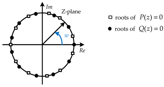
Figure 1.
Illustration of the root location (even).
Combing , Equations (6) and (7) can be described as follows:
2.2. General-Form Polynomial Transformation for the Computation of LSPs Frequencies
The zero crossings of and are the values of LSPs frequencies. In order to find the LSPs frequencies, we need to solve polynomials and .
This paper discusses the commonly used value of = 10, then Equations (12) and (13) can be expressed as a general polynomial:
The above formula can be deployed to a general-form polynomial as follows:
where are the polynomial coefficients, . We define . As is in the range , then is in the range . Therefore, the above two polynomials can be written as
According to Reference [17], the value of can be found by the recursive relations:
where and represent the coefficient of and , respectively. According to Reference [18], we compare Equation (16) with a general-form polynomial (19):
where is a general-form polynomial with the same order of . Comparing Equation (19) to (16), the coefficients relationship of and can be written as
In summary, after a series of steps, LPC polynomials are turned into a general-form polynomial and the relationship between LPC coefficients and general-form polynomial coefficients is found. Therefore, Section 3 introduces the method to solve the general-form polynomial.
3. Polynomial Solution Based on Bairstow Method
As mentioned in Section 2, the LPC polynomials can be transformed into a general-form polynomial. Furthermore, the relationship between the LPC coefficients and coefficients of the general-form polynomial is presented by Equation (20). To solve the general-form polynomial, this paper employs the Bairstow method.
The Bairstow method [18,19,20] is a rapid root-finding algorithm for general-form polynomial. Compared to other conventional methods, it can efficiently reduce the number of addition and multiplication operations, and avoids the evaluation of trigonometric and other complex computations. Thus, the proposed method can converge rapidly and reduce the computation time significantly.
The Bairstow method follows from the observation that the roots of a real quadratic polynomial:
are the roots of a given -order real polynomial
only if can be divided by Equation (21) without the remainder. After deflating, the deflated polynomial can be represented as
where the degree of is -2. The remainder is expressed as . The coefficients of the remainder depend upon and , that is
and the remainder vanishes when and satisfy the condition
According to the scheme, if and are the initial approximations for and , then the iterative process can be written as
where , , , are the partial derivatives with respect to and evaluated at and .
The values and can be found by means of a Horner-type [21] scheme. Comparing Equation (22) with (23), we can get the following recursive formula:
Define , . Combining Equation (27), we can get the following recursive formula:
and the value of and :
The convergence criterion is defined to terminate the iterative procedure when the condition
is satisfied for a specified value . The predefined value determines the accuracy of the root. Then, we can get the root of , assuming there are two distinct roots and ,
To obtain the root of and , we employ a further division of by . Then, we obtain the deflated polynomial:
where the degree of is − 4. To find all the roots, we divide by , where , until the deflation results in a quadratic polynomial.
Table 1 shows the pseudocodes of the proposed method according to Equations (26)–(31). and are the initial value of and , respectively. According to Rererence [18], this algorithm is sensitive to the initial value of and . It will converge rapidly if the initial value of and are sufficiently close to their true values. In Section 4, we will discuss in detail how to choose the initial value of and .

Table 1.
Pseudocode of the proposed method.
After calculating the LSPs with the proposed method, the LSPs should be sorted in descending order according to Equations (10) or (11) with the Insert-Sort [22] algorithm.
Denoting the roots of the general-form polynomial are , the LSPs frequencies are given by , = 1, 2, …, . The values of are ranked as follows:
4. Experiment and Results
4.1. Experimental Environment
As mentioned earlier in Section 2, the LSPs are the representative parameters of the LPC filter. To calculate the LSPs, we use the Aurora data [23] as the benchmark. The Aurora database is a professional speech corpus created by the Aurora project (www.eld.org). There are 1001 clean and 1001 noisy speech files from the Test-A set, spoken by 50 males and 50 females used in this paper.
The test speech signals are sampled at 8 kHz with a resolution of 16 bits per sample. According to Reference [1], the speech signal has a short-term stationary property, so we select every 80 samples (10 ms) as a frame. In order to evaluate the performance of the proposed method, such as computing time, convergence speed, and its impact on speech quality, we choose ITU-T G.729, which is a data compression algorithm using conjugate-structure algebraic-code-excited linear prediction, as a verification platform. The proposed method is implemented using C language and is inserted into the speech encoding module of the ITU-T G.729 platform. Finally, 1,754,330 sets LSPs of 10-order LPC are evaluated on a personal computer (Intel i5-9300H).
4.2. Selection and Update of Initial Values
As introduced in Section 3, the proposed method is sensitive to the selection of the initial values of and , which greatly influences the convergence speed of polynomial optimization. The following experiment shows how to select appropriate initial values.
Three strategies are proposed to select the initial values of and . The first method, called the fixed initial method, which has been employed by a previous works [15], provides fixed initial values for the roots finding. The second method named statistic initial method calculates the statistical mean values of and respectively, then uses the statistical mean values as the initial values for the evaluation of the rest. The third method, called the adaptive initial method, which combines the short-term stationary property of the speech signal, then uses the final result of the current frame as the initial values of the next frame.
Aurora corpus is used as the benchmark set. For the fixed initial method, 1001 speech files from testa_ns_snr15 are evaluated with the initial values being 0, 4 or 8. For the statistic initial method, in order to guarantee the robustness, we use 200 speech files from testa_clean1 as the analytical set, and 1001 speech files from testa_n1_snr15 as the evaluating set, to guarantee the robustness. After the analytical set is processed to satisfy the convergence criterion, the statistic initial method is employed to calculate their statistical mean values and . Then, these values are used to initialize each frame for all speech samples from the evaluating set. For the adaptive initial method, without the necessity of precalculating initializations, 1001 speech files from testa_n1_snr15 are all adopted as the evaluating set. The initial values of the first frame are randomly generated, and the initial values of the subsequent frames are obtained directly from the previous frame.
Table 2 shows a sectional result of the experiment. and are the final converged values of each frame. and represent the differences between the initial values and the final values of and for each frame, respectively. Table 2 shows the and , which are almost lower than 0.03, and Table 3 shows the statistical mean values of and of the 1001 test files. From the table, we know the average values of and are 0.0419 and 0.0305, respectively, and the standard deviation is small. Through the statistical analysis, we discover the value of the parameters between adjacent frames only fluctuates slightly.
Table 2.
The adaptive initial method’s updating principle of and .
Table 3.
The mean and standard deviation of the and .
To investigate the convergence speed of the three initial selection strategies, we perform a statistical analysis of the experiment data. Table 4 and Figure 2 illustrate the average iteration numbers of the fixed, statics and adaptive initial method. Where n1 and n2 mean iteration numbers of the iterative loop for the first five-order polynomial, the iterative loop for the first three-order polynomial, respectively; n3 and n4 mean iteration numbers of the iterative loop for the second five-order polynomial, the iterative loop for the second third-order polynomial, respectively; Total means the iteration numbers for calculating all 10 roots for the two LPC polynomials.The second column of Table 4 means the different initial value for and , where the first row applies and , the second row applies and , and the third row applies and for all test speech frames. In Figure 2, the two vertical lines in each subplot represent the average convergence iterations of the adaptive initial method with the dash, and the static initial method with the dot.
Table 4.
The average iteration numbers of the fixed, statistic and adaptive method for defining the initial values with the same computation accuracy.
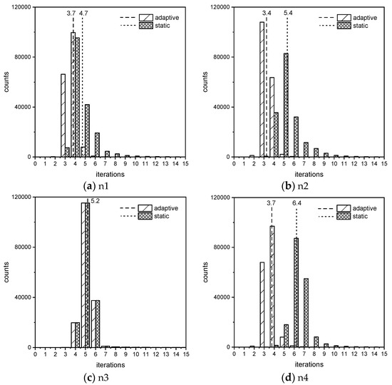
Figure 2.
Histograms of the iteration numbers required to converge, with the adaptive initial method and the static initial method, respectively: (a) n1, (b) n2, (c) n3, and (d) n4.
As Table 4 and Figure 2 show, the setting of the initial values directly affect the convergence iterations. The fixed initial method performs worse than the statistic initial method, and the convergence speed of the adaptive initial method is the fastest, with the average iterations of n1, n2 and n4 at about 3.7, the average iterations of n3 at about 5.2. Further, compared with the fixed initial ( and ) method and statics initial method, the total average iteration numbers are reduced by 68% and 26%, respectively, with the same computation accuracy. This also verifies the conclusion in Table 2; the value of and fluctuate slightly in the adjacent frame due to the short term stationary property of speech signal, thus selecting the final result of and for the current frame as the initial value for the next frame can reduce the average iteration obviously. Therefore, the adaptive initial method is effective, and we apply the adaptive initial method as the selected initial strategy.
4.3. Solve the 10-Order LSP Using the Proposed Method
We randomly select a speech frame to evaluate the computation accuracy of the proposed method. The selection of the initial method follows the strategy mentioned above. We solve the following polynomial and present the experimental results in Table 5, Table 6 and Table 7, where means the jth root of the polynomial, where means the threshold value of iteration termination.
Table 5.
The detail steps to extract the roots of using the proposed method.
Table 6.
Accurate and approximate values determined by the proposed method .
Table 7.
The results of LSP frequencies of .
Table 5 shows the detail steps to solve the polynomial using the proposed method, where means the kth iterative loop. This process includes two stages, of which a 5-order polynomial and a deflated three-order polynomial are both solved in four iterations sequentially. The solving steps of each stage are elaborately illustrated. In the first stage, a five-order polynomial is deflated, where and are the initial value of and in each iteration, respectively, and are calculated by the proposed method after obtaining new values. In the second stage, a deflated three-order polynomial is solved, where and are the initial values in each iteration of the deflated polynomial, and and are the results calculated by the proposed method using and .
Table 6 presents the difference between approximate and accurate values. The third column is the absolute difference between the accurate roots and the approximate roots, where . The experimental results show that the computation accuracy is 0.00001, which means that the approximate values are very close to the accurate ones.
4.4. Performance of the Proposed Method
This section evaluates the performance of the proposed method, including the computation time and the speech quality, by making a comparison between the proposed method and other methods, including the Birge-Vieta method [14], Tschirnhaus Transform [13], original/Modified Ferrari’s method [12], Chen and Wu method [11], Soong and Juang [8], and the Full search.
Due to the lack of the algorithm performance parameters Reference [14], we established the Birge-Vieta method model strictly according to the reference paper. Table 8 shows the Perceptual Evaluation of Speech Quality (PESQ) [24] comparison between the proposed method and the Birge-Vieta method. Table 9 shows the comparison of the average computation time between the proposed method and the previous works, under the same computation accuracy ().
Table 8.
PESQ comparison of the proposed method and the previous methods.
Table 9.
Comparison of the average computation time with the previous works ().
The second column of Table 9 is the average computation time of converting 1,754,330 sets of LPC coefficients to LSF frequencies. Associated Table 7 and Table 8, the results show that the PESQ of the proposed method has improved by 22%, in comparison to the Birge-Vieta method under the testa_clean1, while its computation time is comparable. After normalizing the CPU frequency of system environment to 3.7 GHz and with the same computation accuracy, the proposed method is 17 times faster than the Tschirnhaus transform method, 23 times faster than the Modified Ferrari’s method, 47 times faster than the Original Ferrari’s method, 47.4 times faster than the Chen and Wu method, 152 times faster than the Soong and Juang method, and is 201 times faster than the Full Search. It is obvious that the proposed method is the fastest, with the same computation accuracy.
5. Conclusions
This paper proposed an efficient method to calculate the roots of LPC polynomial, which can transform LPC coefficients to LSPs accurately and rapidly. Associated with the short-term stationary property of speech signal, an adaptive initial method is applied to reduce the average iteration numbers by 26%, as compared with the statics initial method, with the PESQ score reaching 3.35. Experiment results show that the proposed method is 17 times faster than the Tschirnhus Transform, and has a 22% PESQ improvement in comparison to the Birge-Vieta method, with almost the same computation time. Compared to other root-finding methods, the proposed method is the fastest one with comparable speech quality.
Author Contributions
Theory and conceptualization, Y.X.; methodology, Y.X.; software design and development, Y.X.; validation, Y.X.; formal analysis, Y.X. and Z.Z.; investigation, Y.X.; writing–original draft preparation, Y.X.; writing–review and editing, X.F., Z.Z., J.J., Y.Z., Z.Y. and S.Q. All authors have read and agreed to the published version of the manuscript.
Funding
This research received no external funding.
Acknowledgments
I would like to thank Smart sensing R&D center, Institute of microelectronics of Chinese academy of sciences that supported us in this work and Zhejiang University for assistance of the Aurora corpus evaluation.
Conflicts of Interest
The authors declare no conflict of interest.
References
- Rabiner, L.R.; Schafer, R.W. Theory and Applications of Digital Speech Processing; Pearson Education: London, UK, 2011; p. 473. [Google Scholar]
- Makhoul, J. Linear Prediction: A Tutorial Review. Proc. IEEE 1975, 63, 561–580. [Google Scholar] [CrossRef]
- Chowdhury, A.; Ross, A. Fusing MFCC and LPC Features Using 1D Triplet CNN for Speaker Recognition in Severely Degraded Audio Signals. IEEE Trans. Inf. Forensics Secur. 2019, 15, 1616–1629. [Google Scholar] [CrossRef]
- Alku, P.; Saeidi, R. The Linear Predictive Modeling of Speech From Higher-Lag Autocorrelation Coefficients Applied to Noise-Robust Speaker Recognition. IEEE/ACM Trans. Audio Speech Lang. Process. 2017, 25, 1606–1617. [Google Scholar] [CrossRef]
- Ramalho, L.; Fonseca, M.N.; Klautau, A.; Lu, C.; Berg, M.; Trojer, E.; Höst, S. An LPC-Based Fronthaul Compression Scheme. IEEE Commun. Lett. 2017, 21, 318–321. [Google Scholar] [CrossRef]
- Itakura, F. Line Spectrum Representation of Linear Predictive Coefficients of Speech Signals. J. Acoust. Soc. Am. 1975, 57, 535. [Google Scholar] [CrossRef]
- Soong, F.K.; Juang, B.H. Optimal quantization of LSP parameters. IEEE Trans. Speech Audio Process. 1993, 1, 15–24. [Google Scholar] [CrossRef]
- Soong, F.K.; Juang, B.H. Line Spectrum Pair (LSP) and Speech Data Compression. In Proceedings of the IEEE International Conference on Acoustics, Speech, and Signal Processing (ICASSP), San Diego, CA, USA, 19–21 March 1984. [Google Scholar]
- Kang, G.; Fransen, L. Application of line-spectrum pairs to low-bit-rate speech encoders. In Proceedings of the IEEE International Conference on Acoustics, Speech, and Signal Processing (ICASSP), Tampa, FL, USA, 26–29 April 1985; p. 8857. [Google Scholar]
- Kabal, P.; Ramachandran, R.P. The Computation of Line Spectral Frequencies Using Chebyshev Polynomials. IEEE Trans. Acoust. Speech Signal Process. 1986, 34, 1419–1426. [Google Scholar] [CrossRef]
- Wu, C.H.; Chen, J.H. A Novel Two-Level Method for the Computation of the LSP Frequencies Using a Decimation-in-Degree Algorithm. IEEE Trans. Speech Audio Process. 1997, 5, 106–115. [Google Scholar]
- Chen, S.H.; Chang, Y.; Ruan, J.C. An Efficient Computation of LSP Frequencies Using Modified Complex-Free Ferrari Formula. Signal Process. Syst. 2008, 52, 153–163. [Google Scholar] [CrossRef]
- Chen, S.H.; Chang, Y.; Syuan, C.J.Y. The Computation of Line Spectrum Pair Frequencies Using Tschirnhaus Transform. In Proceedings of the International Symposium on Circuits and Systems, Taipei, Taiwan, 24–27 May 2009; pp. 288–291. [Google Scholar]
- Chang, C.H.; Chen, B.W.; Chen, S.H.; Wang, J.F.; Chiu, Y.H. Low-Complexity Hardware Design for Fast Solving LSPs With Coordinated Polynomial Solution. IEEE Trans. Large Scale Integr. Syst. 2015, 23, 230–243. [Google Scholar] [CrossRef]
- Luk, W.S. Finding roots of real polynomial simultaneously by means of Bairstow’s method. Bit Numer. Math. 1996, 36, 302–308. [Google Scholar] [CrossRef]
- Hsiao, C.C.; Brodersen, R. A multi-rate root LPC speech synthesizer. In Proceedings of the IEEE International Conference on Acoustics, Speech, and Signal Processing (ICASSP), San Diego, CA, USA, 19–21 March 1984; pp. 41–44. [Google Scholar]
- Coding of Speech at 8 kbit/s Using Conjugate-Structure Algebraic-Code-Excited Linear Prediction (CS-ACELP); International Telecommunication Union: Geneva, Switzerland, 1996.
- Stoer, J.; Bulirsch, R. Introduction to Numerical Analysis, 2nd ed.; Springer Science & Business Media: Berlin, Germany, 2013; pp. 333–335. [Google Scholar]
- O’Donnell, J. A System for very low data rate speech communication. In Proceedings of the IEEE International Conference on Acoustics, Speech, and Signal Processing (ICASSP), Atlanta, GA, USA, 30 March–1 April 1981; pp. 8–11. [Google Scholar]
- Rothweiler, J. On polynomial reduction in the computation of LSP frequencies. IEEE Trans. Speech Audio Process. 1999, 7, 592–594. [Google Scholar] [CrossRef]
- Hildebrand, F.B. Introduction to Numerical Analysis, 2nd ed.; McGraw-Hill: New York, NY, USA, 1974; pp. 613–618. [Google Scholar]
- Wikipedia. Available online: https://en.wikipedia.org/wiki/Insertion_sort (accessed on 15 January 2020).
- Aurora Corpus. Available online: http://portal.elda.org/en/catalogues/free-resources/free-lrs-set-1/ (accessed on 15 January 2020).
- International Telecommunication Union. Perceptual Evaluation of Speech Quality (PESQ): An Objective Method for End-to-End Speech Quality Assessment of Narrow-Band Telephone Networks and Speech Codecs; International Telecommunication Union: Geneva, Switzerland, 2001. [Google Scholar]
© 2020 by the authors. Licensee MDPI, Basel, Switzerland. This article is an open access article distributed under the terms and conditions of the Creative Commons Attribution (CC BY) license (http://creativecommons.org/licenses/by/4.0/).