SRMM: A Social Relationship-Aware Human Mobility Model ^†

Abstract

Since human movement patterns are important for validating the performance of wireless networks, several traces of human movements in real life have been collected. However, collecting data about human movements is costly and time-consuming. Moreover, multiple traces are demanded to test various network scenarios. As a result, a lot of synthetic models of human movement have been proposed. Nevertheless, most of the proposed models were often based on random generation, and cannot produce realistic human movements. Although there have been a few models that tried to capture the characteristics of human movement in real life (e.g., flights, inter-contact times, and pause times following the truncated power-law distribution), those models still cannot reflect realistic human movements due to a lack of consideration for social context among people. To address those limitations, in this paper, we propose a novel human mobility model called the social relationship–aware human mobility model (SRMM), which considers social context as well as the characteristics of human movement. SRMM partitions people into social groups by exploiting information from a social graph. Then, the movements of people are determined by considering the distances to places and social relationships. The proposed model is first evaluated by using a synthetic map, and then a real road map is considered. The results of SRMM are compared with a real trace and other synthetic mobility models. The obtained results indicate that SRMM is consistently better at reflecting both human movement characteristics and social relationships.

1. Introduction

Human movement patterns greatly affect the performance of various wireless networks, such as opportunistic mobile social networks and delay-tolerant networks, which rely on human movement for pairwise contacts between two communicating devices. Therefore, to fully validate such services and networks, various realistic human movement patterns should be considered. Unfortunately, collecting real-life human movements in various situations is highly time consuming and costly, and it may be infeasible at a very large scale (e.g., citywide or countrywide). That leads to a limited number of available real traces. Therefore, synthetic models for human movement generation are mostly used.

As a result, a lot of synthetic models have been proposed. For instance, the Markovian waypoint model [1] and the random direction model [2] have been used for a long time. A major disadvantage of those models is that they are based on purely random generation of human movement. Thus, the context in real life (e.g., people usually visit their friends, and the places people visit are related over days) were not considered. That causes significant disagreement between the output of mobility models and human movements in the real world.

Recently, several studies have seriously analyzed real human movement traces and found interesting human movement characteristics where flights, inter-contact times (ICTs), and pause times follow truncated power-law distributions [3,4]. Inspired by these studies, a few mobility models, such as the self-similar least-action walk (SLAW) [5] and the working day movement model [6], studied to capture human movement characteristics. However, such models did not consider the social context among people. Therefore, they could not fully reflect human movement in real life.

Social relationships among people are an interesting way to construct mobility models (e.g., community-based mobility model (CMM) [7], home-cell community-based mobility model (HCMM) [8]). Such models consider social context. For example, people prefer to visit places where many of their friends are staying. Nevertheless, the models did not consider human movement characteristics (e.g., flights, ICTs, the radius of gyration, and pause-time distributions). Additionally, selecting the destinations of people is only affected by their social ties without considering important contexts (e.g., in real life, the places an individual visit during different day trips are correlated, and people tend to visit nearby places). For those reasons, such models could not reflect realistic human movement.

To address the limitations in existing models, we propose a new human mobility model called the social relationship–aware human mobility model (SRMM), which takes into account social relationships among people and human movement characteristics.

Specifically, SRMM considers the characteristics of human movements in terms of flights, ICTs, the radius of gyration, and pause-time distributions. A flight is defined as a Euclidean distance between two consecutive spots visited by an individual. Spots are the geographic positions in which a person stays for longer than a certain amount of time. Studies have shown that the distribution of flights follows truncated power-law distributions [3,4]. ICT represents the time elapsed between two successive contacts for a given pair of people. Freeman investigated real-life human movements and reported that the ICTs of people in real life can be reproduced in truncated power-law distributions [9]. The next characteristic is the radius of gyration, which indicates the spatial extent of a person’s trajectory during an observation period. According to work by Gonzalez et al. [3], the radius of gyration can also be modeled by truncated power-law distributions. Finally, pause time (the sojourn time of a person in one spot) was analyzed [4,10]. The obtained results demonstrated that pause times during movement have truncated power-law distributions. SRMM captures the truncated power-law distributions of flights, ICTs, the radius of gyration, and pause times.

In SRMM, the social characteristics of humans are also considered. Our model takes a social graph as input, which represents the relationships among people, followed by a clustering algorithm that partitions people into social groups. Each social group represents a community in the real world, such as a family, a class, or a football team. Then, spots to be visited by people are generated and grouped into places, i.e., a place (e.g., a mall) consists of multiple spots (e.g., clothing stores, the cafeteria, and restrooms). We use the observation that people in the same community usually visit similar places. For instance, the members of a football team often visit the same places, such as the stadium, the canteen, and the dressing rooms. SRMM chooses a group of frequently visited places for a social group. As a result, the people in a social group will have the same frequently visited places. Then, each person chooses frequently visited spots from frequently visited places.

Our model also considers scenarios where people sometimes visit a new place (different from places other members in the same social group visited) by adding randomly visited spots for each person at the beginning of each day. The frequently visited spots and the randomly visited spots for a person are defined as candidate spots.

During daily trips, each person selects destinations from his/her candidate spots. To select destinations, human movement properties and social relationships are considered. In SRMM, a person selects a destination based on the distance from the person’s current location and the number of social acquaintances they have (i.e., people from the same social group) in those places. Specifically, a place that is a shorter distance away and that accommodates a larger number of social acquaintances has a higher probability of being visited.

To validate human movement characteristics, the characteristics of the proposed model are collected on two maps (i.e., a synthetic map and a real road map). In the case of the synthetic map, the real mobility trace [11] on the New York City area is considered. Based on the extracted information (e.g., the number of spots and the dispersion of spots) from the real trace, a synthetic map is generated. Then, the movement trace of SRMM on the synthetic map is compared with the real mobility trace [11] and synthetic traces generated by other mobility models. The movement trace of SRMM is also collected on a real road map of Helsinki downtown [12]. Since there are no available real mobility traces in case of the real road map of Helsinki downtown, the results are compared between synthetic mobility models. SRMM provides human movement characteristics that closely approximate real movements and that are well-matched to truncated power-law distributions. Also, reflections of social relationships in the mobility model are evaluated. The obtained results show that SRMM accurately reflects social relationships.

In summary, the main contributions of this paper are listed as follows:

• First, most of existing mobility models do not consider human movement characteristics. Even though a few mobility models take into account human movement characteristics, they lack consideration for social relationships on human movements. Therefore, realistic human movement patterns cannot be presented. To address this problem, SRMM reflects both human movement characteristics and social relationships on human movements. Specifically, we take into account the characteristics of human movements in terms of flights, ICTs, the radius of gyration, and pause-time distributions. Moreover, social contexts in human movement (e.g., people in the same community usually visit similar places; people prefer to visit places where many of their friends are staying) are also considered.
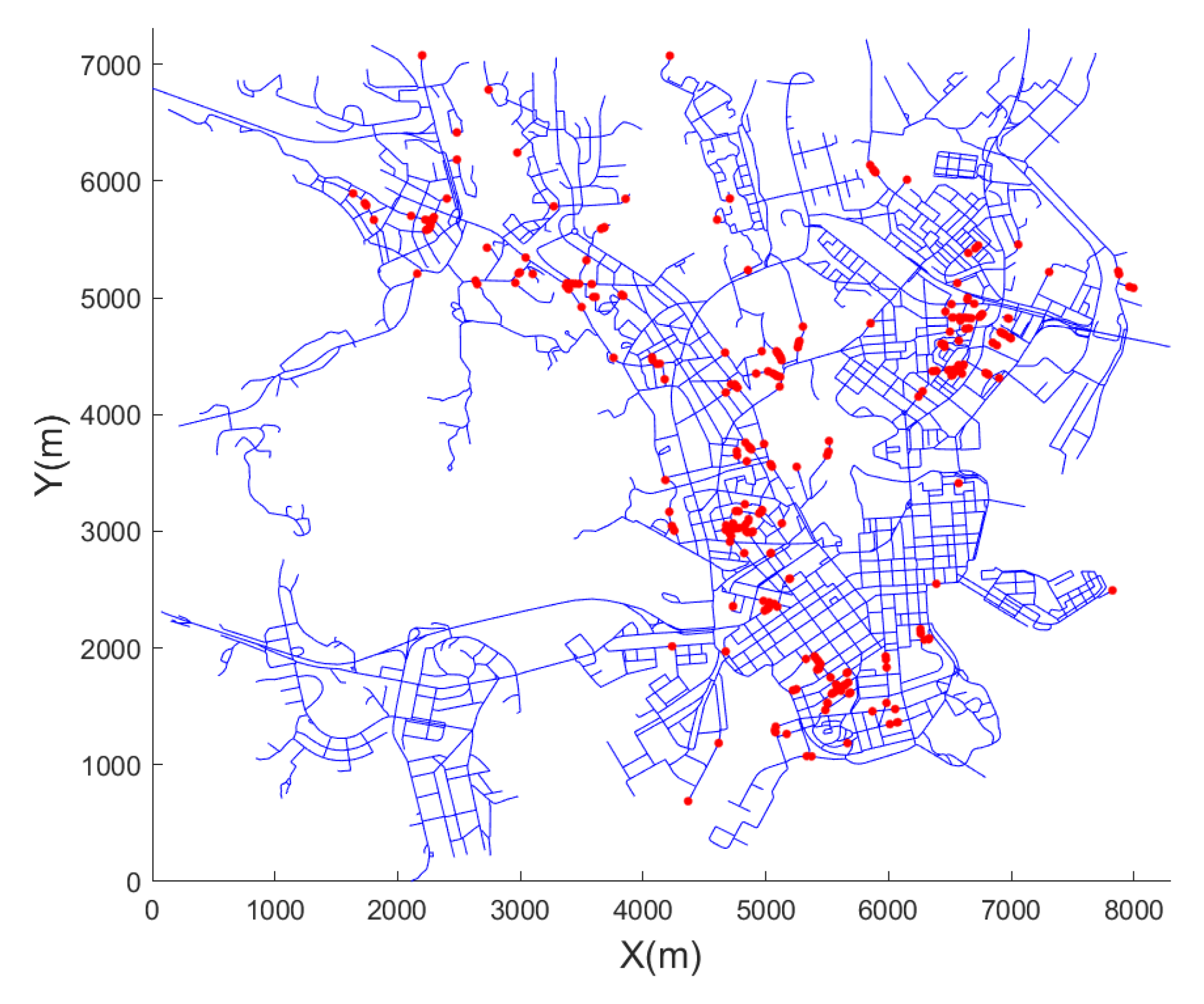
• Second, to better approximate realistic environments when validating mobility models, mobility models are simulated not only on a synthetic map but also on a real road map (i.e., a real road map of Helsinki downtown [12]). Various experiments are conducted to validate mobility models.
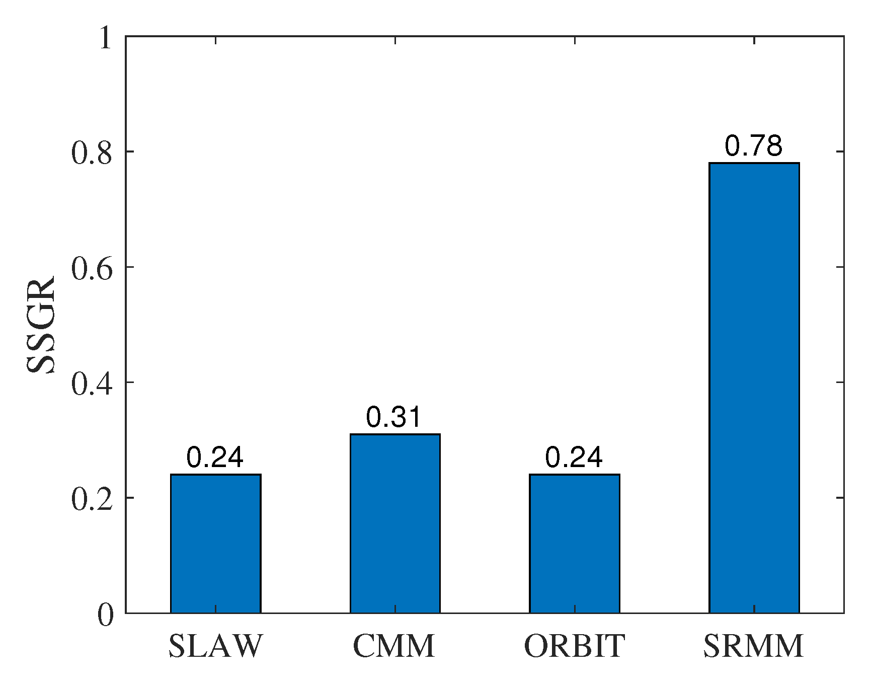
• Third, various metrics are used to validate human movement characteristics. Specifically, Kullback—Leibler divergence [13], Kolmogorov—Smirnov test [14], and weighted mean relative difference [15] are used to show how well the human movement characteristic generated by mobility models match a real trace. Then, Akaike information criterion and Bayesian information criterion [16] are used to validate the fitting of the human movement characteristics with truncated power-law distributions. To evaluate the reflection of social relationships, a new performance metric, called the same social group ratio (SSGR), is proposed. The obtained results indicate that human movement characteristics from SRMM are close to the real trace and SRMM is the best to reflect social relationships.

The rest of this paper is organized as follows. First, Section 2 discusses background. Then, Section 3 describes SRMM in more detail. The implementation and performance of the SRMM model are discussed in Section 4. Finally, in Section 5, we conclude this paper.

2. Background

2.1. Preliminaries

In this part, the terms used in our paper are presented. First, Kullback–Leibler (KL) divergence [13], Kolmogorov-Smirnov (K-S) test [14], and weighted mean relative difference (WMRD) [15], which measure the similarity between two distributions, is described. Then, the model selection criteria (i.e., the Akaike information criterion [16] and the Bayesian information criterion [16]) are considered.

2.1.1. Kullback–Leibler Divergence

To measure how a probability distribution diverges from another distribution, Kullback et al. [13] introduced KL divergence. This value can show the directed divergence and can measure the distance between two probability distributions. A lower value for KL divergence indicates that two distributions are more similar. Let P and Q be two probability distributions. The KL divergence of Q from P is denoted as $D_{KL}(P||Q)$.

For discrete probability distributions $P(i)$ and $Q(i)$, $D_{KL}(P||Q)$ is defined as follows [17]:

$$D_{KL}(P||Q)=\sum _{i}P(i)\log {\displaystyle \frac{P(i)}{Q(i)}}$$

(1)

In practice, it may incur a log of zero. To avoid this, all probabilities have a small positive constant added.

2.1.2. Kolmogorov-Smirnov Test

Two-sample K-S test [14] is used to measure the similarity between two distributions of two data samples. Let $\mathit{X}$ and $\mathit{Y}$ be the two given data samples. The cumulative distribution function of $\mathit{X}$ and $\mathit{Y}$ are denoted as $F_x(i)$ and $F_y(i)$, respectively. D denotes the K-S statistic. D is defined as:

$$D=ma{x}_i|F_x(i)-F_y(i)|$$

(2)

$h_0$ is a null hypothesis that data sample $\mathit{X}$ and data sample $\mathit{Y}$ come from the same distribution. $\mu$ defines a significance level. For a given $\mu$ value, a critical value can be obtained from a table in [14]. Let $D_{\mu }$ be the critical value for level $\mu$. If $D\le D_{\mu }$, $h_0$ is accepted at significance level $\mu$. The maximum value of significance level $\mu$, which still satisfies the condition $D\le D_{\mu }$, is defined as P value. In other words, if $\mu \le P$, $h_0$ is accepted. P value can show the possibility that two samples come from the same distribution. A higher P value means that distributions of two data samples are more similar.

2.1.3. Weighted Mean Relative Difference

Weighted mean relative difference (WMRD) [15] is used to compare the difference between two probability distributions. Let P and Q be two probability distributions. WMRD between P and Q is defined as follow:

$$WMRD={\displaystyle \frac{{\sum }_i|P(i)-Q(i)|}{{\sum }_i{\displaystyle \frac{P(i)+Q(i)}{2}}}}$$

(3)

WMRD value presents the difference between two probability distributions. A higher WMRD value means that two probability distributions are more different. In other words, two probability distributions are more similar if WMRD between them is low.

2.1.4. Model Selection Criteria

We assume that there are a given dataset and a set of models. Then, model selection criteria can be used to find the best model to match the given dataset. In this paper, we use the Akaike information criterion (AIC) and the Bayesian information criterion (BIC).

To calculate AIC and BIC, maximum likelihood estimation (MLE) [18] is used first to find an estimator that maximizes the likelihood function [18]. Let $\mathit{D}$ be the given data set. A model has probability distribution f by unknown parameter $\mathit{\lambda }$, which could be a vector. $L(\mathit{\lambda }|\mathit{D})$ denotes the likelihood function of the model with data $\mathit{D}$. $L(\mathit{\lambda }|\mathit{D})$ is defined as:

$$L(\mathit{\lambda }|\mathit{D})=\prod _{i\in \mathit{D}}f(i|\mathit{\lambda })$$

(4)

MLE finds an estimator $\widehat{\mathit{\lambda }}$ that maximizes the likelihood function.

• AIC is the model selection criterion established by a relationship between KL divergence and MLE. The quality of the models is estimated by AIC values. A lower AIC value indicates that the model is a better fit to the given data. Let us define the number of estimated parameters to be $n_{\mathit{\lambda }}$. The AIC is calculated as:

  $$AIC=-2\log (L(\widehat{\mathit{\lambda }}|\mathit{D}))+2n_{\mathit{\lambda }}$$

  (5)
• BIC is another model selection criterion based on information theory but set within Bayesian context. The model with the lowest BIC is preferred. Let $n_{\mathit{D}}$ be the number of data samples in $\mathit{D}$. BIC is defined as:

  $$BIC=-2\log (L(\widehat{\mathit{\lambda }}|\mathit{D}))+n_{\mathit{\lambda }}\log (n_{\mathit{D}})$$

  (6)

2.2. Related Work

In this section, the ways to collect human movements are presented. Then, we briefly present the existing mobility models, the human characteristics they capture, and the limitations of those models.

Real human movements are mostly recorded from opportunistic contacts between people using wireless devices in small areas, such as offices, conferences, and campuses. In recent years, several real traces have been collected [11,19,20,21]. Rhee et al. [11] used Garmin GPS 60CSx handheld receivers to collect human movements from five different sites (i.e., campuses of North Carolina State University, Korea Advanced Institute of Science and Technology, New York City, Disney World, and the North Carolina state fair). McNett and Voelker, [19] used 300 wireless handheld PDAs running Windows CE to record WiFi access point information over 11 weeks. Scott et al. [20] released a dataset that included five trace sets of Bluetooth sightings by groups of people carrying iMote devices. In Sensible DTU [21], $1000$ smartphones are distributed to participants who volunteered for the study. Custom software is installed on each smartphone to record useful data (e.g., location, Bluetooth scans, WiFi scans).

However, collection of human movements in real life is infeasible on a very large scale and not flexible for configuring a network. It also takes a lot of resources, such as time, money, and human effort. These reasons have resulted in a limited number of available real traces. As a result, numerous synthetic models were studied to overcome the limitations. To produce movements similar to human movements in real life, the model must capture human movement characteristics (e.g., pause times, flights, the radius of gyration, and ICTs) and correlate them with the social relationships of people.

In early works, most mobility models were based on pure random generation of movements [1,2]. In the Markovian waypoint mobility model [1], people randomly selected destinations and pause times. The random direction model [2] randomly chooses directions of human movements. Most parameters are based on random generation without consideration of social relationships and human movement characteristics. Therefore, such models lack the regular patterns shown in daily human walks.

There are several mobility models based on human movement characteristics [5,6,22,23,24,25,26]. For instance, in SWIM [25], the human movement characteristics are considered, and the truncated power-law distribution of ICTs is produced. In SLAW [5], spots are generated in the area and grouped into places. Then, each person selects a list of places and picks several spots in these places to visit. Selection of destinations is based on distance from the person to those spots. A spot with at a shorter distance has a higher probability of being selected. SLAW produced truncated power-law distributions of flights, ICTs, and pause times. In SMOOTH [22], theme park mobility model [23], and urban context aware mobility model [24], they also considered truncated power-law distributions of flights, ICTs, and pause times, whereas in the working day movement model [6], contact time and ICT distributions closely followed the ones found in traces from real-world measurement experiments. Royer et al. [26] analyzed national household travel survey data [27] to generate streets, avenues, and addresses in the simulation area. At the beginning of the trip, each person has an agenda that covers all day-long activities for the person. Each item on the agenda indicates when, where, and what activity the person is going to participate in. However, these models lacked consideration for the social context in human movement. Therefore, they could not completely approximate realistic human movements.

Inspired by social context, several mobility models were studied [7,8,28,29,30]. At first, studies were based on simple contexts, as done in CMM [7] and HCMM [8]. In CMM, the simulation area is divided into several sub-areas, and people are grouped into communities by using social relationship information. Then, each community is randomly associated with a sub-area. The attractiveness of each sub-area is determined by the current number of people in that area. HCMM retains the social model in CMM and improves on it by adding a new concept: the home cell of each person. Specifically, the attractiveness of the home cell to home-cell owners is maintained. In CMM and HCMM, selection of destinations is only affected by social relationships, which lack many regular patterns of human movements in real life (e.g., people are attracted by popular places and prefer visiting nearby places). In the sociological orbit aware location approximation and routing mobility model (ORBIT) [28], places are randomly generated in the given area, and then each person is assigned to a subset of places. A person moves around the assigned places and selects the next destination at random. As a result, the visited places for different people are not correlated, and visited places for people in real life are not considered to reproduced. Therefore, realistic human movement patterns cannot be presented.

To more accurately approximate the social context, in the sociological interaction mobility for population simulation model [29], a person’s decision to move to a place is separated into two modes. The socialize mode is the movement toward acquaintances, and the isolate mode is intended for an escape from undesired situations. In particular, if the number of individuals in a person’s current location is within a preset comfort range, the person will feel comfortable in this place and will be in socialize mode. By contrast, if the number of individuals in that place exceeds the comfort range, the person will be in isolate mode. Yang et al. [30] proposed a mobility model in which a person can belong to overlapping communities and a difference of communities in each time period. Then, each community is randomly associated with a set of places, and people randomly select destinations to visit from associated places. Those models do well in capturing the social characteristics of people. Unfortunately, they still have limitations due to a lack of consideration for human movement characteristics.

Our proposed model addresses the limitations in the existing models. We reproduce characteristics of human movement (i.e., the distributions of flights, ICTs, radii of gyrations, and pause times all follow power-law distributions), and we reflect the social context of human movement.

3. Social Relationship–aware Human Mobility Model

In this section, the model for SRMM is presented. Then, SRMM is described in four phases. In phase 1, people are partitioned into social groups by using information from a social graph. In phase 2, we describe how spots are generated and grouped into places. The candidate places and the candidate spots are selected in phase 3. Finally, in phase 4, the destination spots for people are determined.

3.1. Model

In our problem, human movements are reproduced in a considered area. In this area, we assume there is a set of places, ${\mathbb{S}}_P=\{P_i|1⩽i⩽n_P\}$, where $n_P$ is the number of places. Each place, $P_i$, consists of multiple spots. Let the set of spots in the considered area be ${\mathbb{S}}_s=\{s_i|1⩽i⩽n_s\}$, where $n_s$ is the number of spots. In other words, place $P_i$ is an area (e.g., mall, park, or hotel) that includes a set of spots. A spot, $s_i$, is a staying point on the map, such as a clothing store in a mall, or a bench in a park.

Among all people, social relationships exist that affect human movements. We partition people into social groups that represent realistic communities, such as groups of friends, families, and football teams. Each group includes people, who have close relationships. In the considered area, we denote the set of people as ${\mathbb{S}}_u=\{u_i|1⩽i⩽n_u\}$ and the set of social groups as ${\mathbb{S}}_G=\{G_i|1⩽i⩽n_G\}$, where $n_u$ and $n_G$ are the number of people and the number of groups, respectively. Several regular patterns are usually present in human movements. For example, people tend to visit their friends and visit popular places where there are many spots. Each individual prefers to visit certain places, rather than other places. Details of definitions of sets can be found in

Table 1. Definitions of Sets.

${\mathbb{S}}_P=\{P_i|1⩽i⩽n_P\}$	The set of places
${\mathbb{S}}_s=\{s_i|1⩽i⩽n_s\}$	The set of spots
${\mathbb{S}}_u=\{u_i|1⩽i⩽n_u\}$	The set of people
${\mathbb{S}}_G=\{G_i|1⩽i⩽n_G\}$	The set of social groups
${\mathbb{S}}_{FP}^u$	The set of frequently visited places for person u
${\mathbb{S}}_{FS}^u$	The set of frequently visited spots for person u
${\mathbb{S}}_{RP}^u$	The set of randomly visited places for person u
${\mathbb{S}}_{RS}^u$	The set of randomly visited spots for person u
${\mathbb{S}}_{CP}^u={\mathbb{S}}_{FP}^u\cup {\mathbb{S}}_{RP}^u$	The set of candidate places for person u
${\mathbb{S}}_{CS}^u={\mathbb{S}}_{FS}^u\cup {\mathbb{S}}_{RS}^u$	The set of candidate spots for person u

.

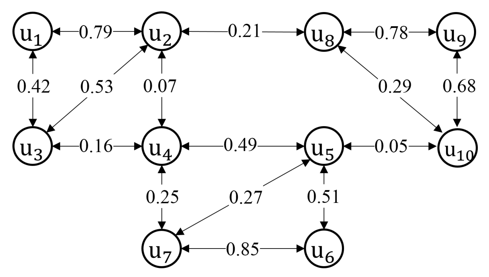
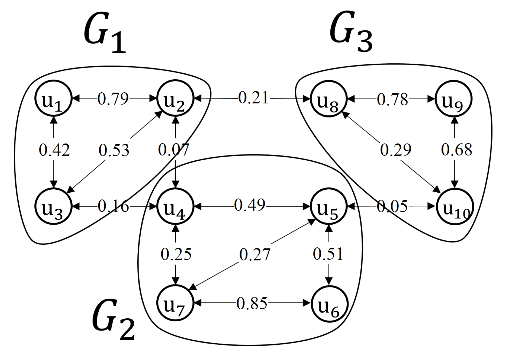
3.2. Phase 1: Human Grouping

In this phase, a clustering algorithm is used to detect social groups in a social graph, which is provided as input.

The social graph illustrates the strengths of closeness among people. The strength of social closeness between two people is assumed to be in the range [0,1]. Figure 1 shows an example of a social graph with 10 people $(u_1,u_2,\dots ,u_{10})$. The strength between $u_1$ and $u_2$ equals 0.79, whereas the strength between $u_5$ and $u_{10}$ equals 0.05. There is no connection link between $u_5$ and $u_8$. This implies that the strength is 0. The social graph can also be presented as a matrix where the entries are the closeness strengths among the people.

For detection of social groups in the input social graph, we use a spectral clustering algorithm [31]. The spectral clustering algorithm is simple to implement in practice and usually outperforms traditional algorithms such as the K-means algorithm [32]. Recall that $n_G$ is the number of social groups, and $n_u$ is the number of people. By using the spectral clustering algorithm, people who have strong relationships will be grouped in a social group. From $n_u$ people, $n_G$ social groups are generated. Specifically, the spectral clustering algorithm uses the social matrix and $n_G$ as the inputs. Based on the social matrix, a Laplacian matrix is constructed by using a symmetric normalized technique [33]. After that, we calculate the set of eigenvectors for the Laplacian matrix. Then, people are represented in a lower-dimensional space, $R^{n_u\times n_G}$, which is formed by the first $n_G$ eigenvectors that correspond to the $n_G$ lowest eigenvalues. At the final step of the spectral clustering algorithm, the K-means algorithm is used on this data space to obtain social group set ${\mathbb{S}}_G=\{G_i|1⩽i⩽n_G\}$. Each social group $G_i$ includes a set of people.

An example of the clustering result is shown in Figure 2. We obtain social group set ${\mathbb{S}}_G=\{G_1,G_2,G_3\}$ from the social graph, where $G_1$ includes $u_1,u_2,u_3$; $G_2$ includes $u_4,u_5,$$u_6,u_7$; and $G_3$ includes $u_8,u_9,u_{10}$.

3.3. Phase 2: Generation of Spots

In this phase, spots in ${\mathbb{S}}_s$ are generated in the area and then grouped into places. Lee et al. [34] reported that visited spots of human in real life can be reproduced as fractal spots. This means that people always tend to gather in popular places, which conforms to contexts in real life, such as homes, parks, schools, and workplaces. To generate fractal spots, SRMM uses the bursty spot model (BSM) [34]. From real trace data [11], the real-spot distribution for New York City is shown in Figure 3a, and an example of a synthetic map obtained by using BSM is displayed in Figure 3b. As shown in the figures, the dispersion of spots on the synthetic map is similar to the real map.

After generating a synthetic map with fractal spots, the set of places, ${\mathbb{S}}_P=\{P_i|1⩽i⩽n_P\}$, is formed by grouping spots in circles with radius r in meters. For example, to form place $P_i$, a spot is selected as the center of place $P_i$. To select the center spot, spots are considered one by one in increasing order of X-coordinates of spots. In the case that X-coordinates of spots are equal, spots in increasing order of Y-coordinates of spots are considered. If a spot does not belong to any places, it will be selected as the center spot of place $P_i$. Then, spots, which are within a radius of r meters from the center spot and do not belong to any places, will be grouped into place $P_i$. In this way, place $P_i$ includes a set of spots within a range of r meters. The selection of r value is based on the transmission range of wireless personal area networks.

3.4. Phase 3: Selection of Candidate Places and Candidate Spots

In this phase, each social group is associated with a set of places. The associated places are called frequently visited places. Then, each person in the same social group selects a set of spots from their frequently visited places to obtain their frequently visited spots. Let G be a social group in ${\mathbb{S}}_G$ and u be a person in G. The set of frequently visited places and the set of frequently visited spots for person u are denoted as ${\mathbb{S}}_{FP}^u$ and ${\mathbb{S}}_{FS}^u$, respectively.

In addition, at the beginning of each day trip, each person newly selects another place as a randomly visited place, then picks several spots in this place as randomly visited spots. Let ${\mathbb{S}}_{RP}^u=\{R{P}^u\}$ be the set of randomly visited places for person u, where $R{P}^u$ is the randomly visited place of person u. The set of randomly visited spots of person u is denoted ${\mathbb{S}}_{RS}^u$.

On a day trip, ${\mathbb{S}}_{CP}^u={\mathbb{S}}_{FP}^u\cup {\mathbb{S}}_{RP}^u$ is the set of candidate places for person u, and ${\mathbb{S}}_{CS}^u={\mathbb{S}}_{FS}^u\cup {\mathbb{S}}_{RS}^u$ is the set of candidate spots for person u.

The operation of this phase is presented in three steps as follows:

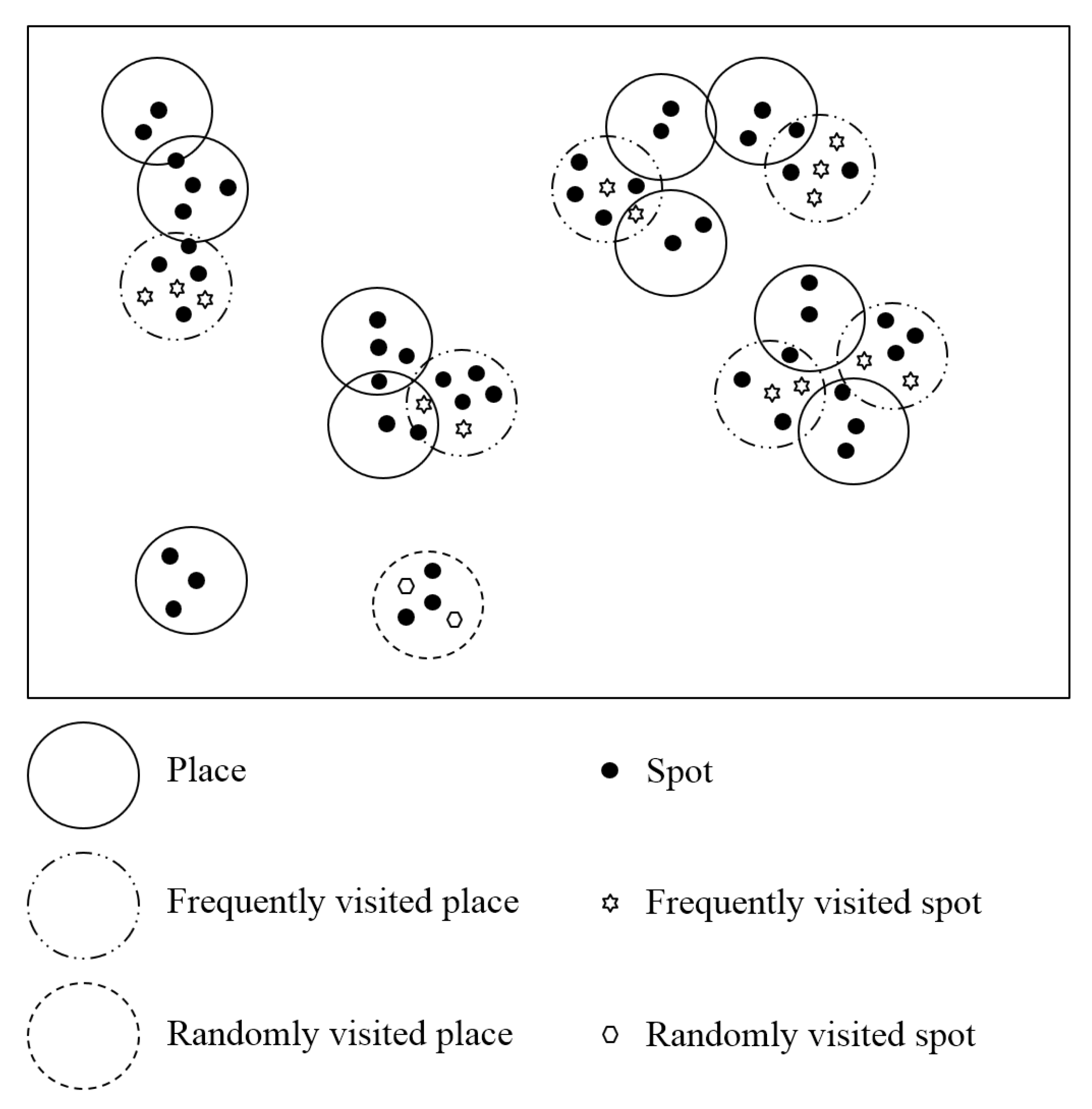
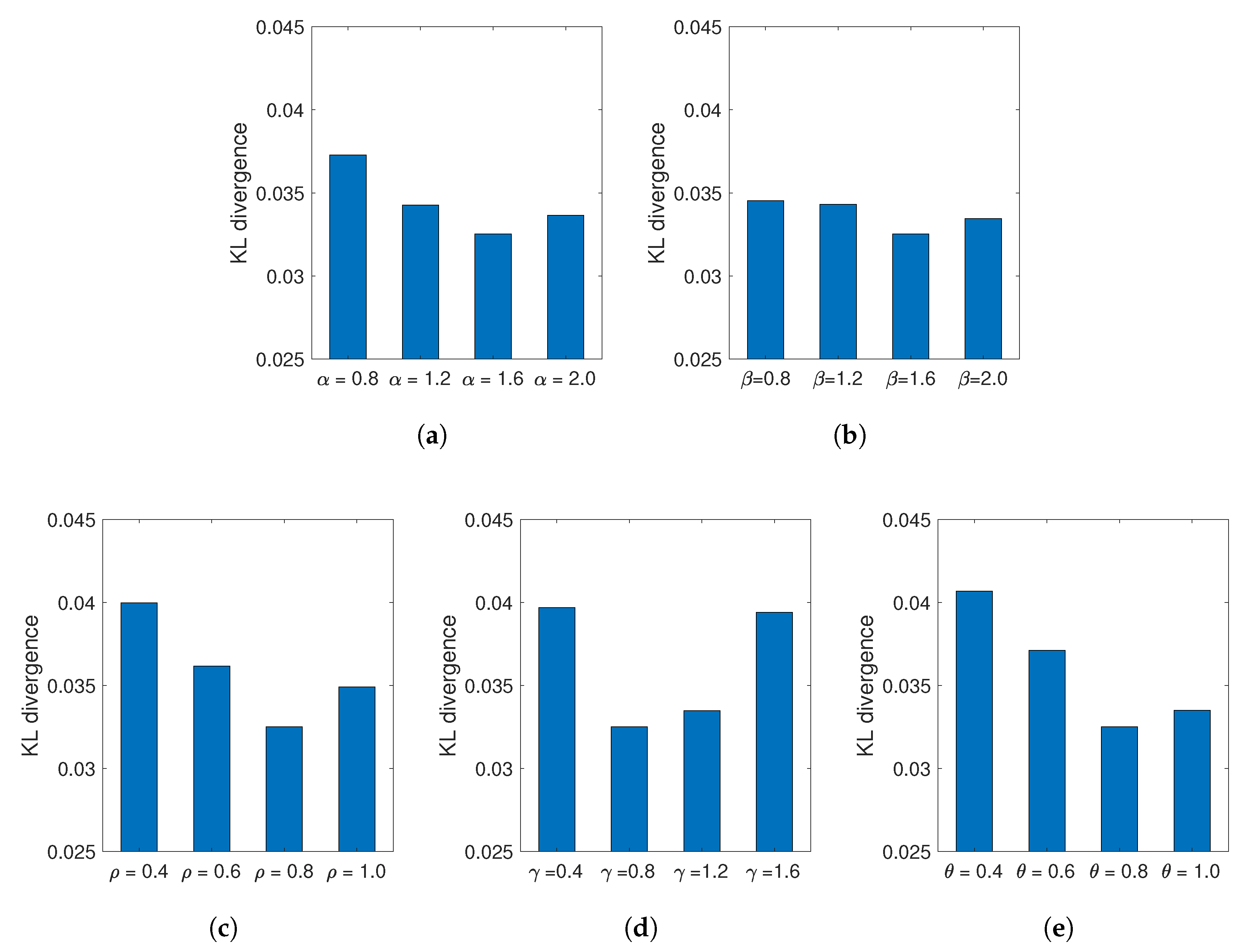
• Step 1: Selecting frequently visited places
  People in a social group often visit the same places. That is a common context in real life. For example, a group of friends usually visits the same mall, park, and restaurant. In SRMM, each social group is associated with several places called frequently visited places. Accordingly, people in the same social group have the same frequently visited places. We define random variable x as the number of frequently visited places selected for a social group. Let A be a place in ${\mathbb{S}}_P$, and $n_s^A$ denotes the number of spots in place A. Let $P_{G,A}$ be the probability that social group G selects place A as a frequently visited place. $P_{G,A}$ is calculated as:

  $$\begin{array}{c}\hfill P_{G,A}={\displaystyle \frac{{(n_s^A)}^{\theta }}{{\sum }_{i\in {\mathbb{S}}_P}{(n_s^i)}^{\theta }}}\end{array}$$

  (7)

  where $\theta$ ($\theta >0$) is a parameter that adjusts the effect of the number of spots in selecting frequently visited places. Equation (7) indicates that a place with more spots has a higher probability of being selected. That agrees with the context in real life whereby most people prefer visiting popular places with more popularly visited points, rather than unpopular places. A higher $\theta$ also implies that several places with more spots will be frequently selected by social groups. In contrast, a lower $\theta$ value will reduce the possibility that different social groups will select the same frequently visited places.
• Step 2: Selecting frequently visited spots
  We define random variable y $(0\le$y$\le 100\%)$ as a percentage value. After obtaining the set of frequently visited places (${\mathbb{S}}_{FP}^u$), person u randomly picks y percent of the spots from each place in ${\mathbb{S}}_{FP}^u$ as frequently visited spots (where person u usually visits during day trips).
• Step 3: Selecting a randomly visited place and randomly visited spots on a day trip
  To match the context of real life (on a day trip, a person visits not only frequently visited spots but additional spots, on occasion), this step randomly selects a new place and new spots at the beginning of each day.
  First, social group G randomly selects several new places. The number of new places is denoted as z. Then, person u randomly chooses a place from the z newly selected places as the randomly visited place ($R{P}^u$), and picks y percent of the spots in $R{P}^u$ to obtain randomly visited spots.

The values of random variables x, y, and z in this phase are assumed to follow truncated normalized distributions. The distributions of these random variables can be adjusted to reflect various situations in real life. For example, people living in an urban area have more visited places and visited spots than people living in a mountain area.

Now, the candidate places and the candidate spots are obtained. An example of chosen places and spots for person u is shown in Figure 4.

3.5. Phase 4: Selection of the Destination Spots

In this step, person u first randomly chooses a spot in $S_{FS}^u$ as the home spot. Each day person u starts the trip from this spot. The home spot for person u is denoted as $h^u$. Then, from ${\mathbb{S}}_{CP}^u$ obtained in phase 3, person u selects a place to visit. Let $S{P}^u$ denote the selected place. Finally, person u selects a destination spot from the candidate spots in place $S{P}^u$.

Now, the process for selecting the destination spot of person u is presented in detail. This process comprises two steps.

• Step 1: Person u selects place $S{P}^u$ from set ${\mathbb{S}}_{CP}^u$ to visit
  Based on the assumption that people usually prefer visiting nearby places rather than faraway places, and they are also attracted to places where many of their friends are visiting, SRMM considers two components (the distances from the places to person u’s current location, and the social relationships of person u) while selecting place $S{P}^u$ from set ${\mathbb{S}}_{CP}^u$.
  Let i be an arbitrary place in ${\mathbb{S}}_{CP}^u$. To obtain the probability that person u visits place i, two probability components are used.
  First, we consider the probability related to distance. Let $d_{u,i}$ denote the distance from person u to place i. $P_{u,i}^D$ denotes the probability of selection related to distance. This probability is calculated as:

  $$\begin{array}{c}\hfill P_{u,i}^D={\displaystyle \frac{{\left({\displaystyle \frac{1}{d_{u,i}+c_d}}\right)}^{\alpha }}{{\sum }_{j\in {\mathbb{S}}_{CP}^u}{\left({\displaystyle \frac{1}{d_{u,j}+c_d}}\right)}^{\alpha }}}\end{array}$$

  (8)

  where an adjustment parameter, $\alpha$$(\alpha >0)$, modifies the effect of the distance. To avoid situations where the distance from person u to a place is 0, we use a small constant, $c_d>0$. Equation (8) implies that a place within a shorter distance has a higher value for $P_{u,i}^D$.
  Secondly, we consider the probability of selection related to social relationships. Recall that person u belongs to group G. Let $n_u^{G,i}$ be the number of people, who are currently visiting place i and belong to group G. We define $P_{u,i}^S$ as the probability of selection related to social relationships. $P_{u,i}^S$ is calculated as:

  $$\begin{array}{c}\hfill P_{u,i}^S={\displaystyle \frac{{(n_u^{G,i}+c_s)}^{\beta }}{{\sum }_{j\in {\mathbb{S}}_{CP}^u}{(n_u^{G,j}+c_s)}^{\beta }}}\end{array}$$

  (9)

  where parameter $\beta$$(\beta >0)$ adjusts the effect of social relationships, and a small constant, $c_s>0$, is used to avoid a result where $n_u^{G,i}=0$. Equation (9) indicates that a place with many friends of person u has a higher value for $P_{u,i}^S$.
  Finally, we define $P_{u,i}^{DS}$ as the probability that person u chooses to visit place i. $P_{u,i}^{DS}$ is calculated by combining two components, $P_{u,i}^D$ and $P_{u,i}^S$, as follows:

  $$\begin{array}{c}\hfill P_{u,i}^{DS}=\rho \times P_{u,i}^D+(1-\rho )\times P_{u,i}^S\end{array}$$

  (10)

  where a tunable parameter, $\rho \in [0,1]$, modifies the balance between distance and social relationship.
• Step 2: Person u selects a destination spot in $S{P}^u$
  Let ${\mathbb{C}}_{SP}^u$ denote the set of candidate spots that are in place $S{P}^u$ for person u. In this step, person u selects a spot in ${\mathbb{C}}_{SP}^u$ as the destination spot. Let s be a spot in ${\mathbb{C}}_{SP}^u$, and let $l_{u,s}$ be the distance from person u to spot s. $P_{u,s}$ denotes the probability that person u selects spot s as the destination spot. This probability is calculated as:

  $$\begin{array}{c}\hfill P_{u,s}={\displaystyle \frac{{\left({\displaystyle \frac{1}{l_{u,s}}}\right)}^{\gamma }}{{\sum }_{j\in {\mathbb{C}}_{SP}^u}{\left({\displaystyle \frac{1}{l_{u,j}}}\right)}^{\gamma }}}\end{array}$$

  (11)

  where adjustment parameter $\gamma$$(\gamma >0)$ is used to adjust the effect of the distance. Equation (11) indicates that spots near person u have higher probability values, which also agrees with the real-life context.

In SRMM, everyday person u is assumed to move from 7:00 to 19:00 (i.e., 12 h per day). On a day trip, person u starts moving from home spot $h^u$ and comes back to home spot $h^u$ at $t_c$, i.e., $t_c$ is the homecoming time of person u. The value of $t_c$ is assumed to follow a truncated normalized distribution.

3.6. Complexity Analysis

In this subsection, the time complexity of mobility models is analyzed. Recall that $n_u$ is the number of people in the network and $n_s$ is the number of spots. Let T denote the simulation time. The complexity of SRMM model is as follows. It takes $O(n_u^2)$ time to group human into social groups, $O(n_s)$ time to generate spots and partition spots into places, $O(T\times n_u)$ time to select candidate places and candidate spots, and $O(T\times n_u^2+T\times n_u\times n_s)$ time to select the destination spot. Therefore, the complexity of SRMM model is $O(T\times n_u^2+T\times n_u\times n_s)$. We also analyze the time complexity for SLAW, CMM, and OBRIT mobility model and the time complexities are $O(T\times n_u\times n_s)$, $O(T\times n_u^2)$, and $O(T\times n)$, respectively. The results of complexities show that SRMM takes a longer time than others mobility models since SLAW does not consider social relationships in selecting the destination, CMM does not take into account generating spots in the area and considering the distance in selecting the destination spot, and in ORBIT, the most of steps are random processes.

4. Evaluation Results

In this work, Matlab was used to validate the proposed social relationship–aware human mobility model. We take into account human movement characteristics and social relationships of the mobility model. First, KL divergence, K-S test, WMRD are used to show how well the human movement characteristics generated by the mobility model match a real trace. Then, to validate the fitting of the human movement characteristics with truncated power-law distributions, AIC and BIC values are used. Finally, a new performance metric (the same social group ratio) is used to evaluate the reflection of social relationships. The results obtained with SRMM are compared with the results from SLAW [5], CMM [7], and ORBIT [28].

4.1. Simulation Setup

Let T denote simulation time. As many as movements of 100 people for $T=200$ h are generated. According to results shown in [35], the movement speed of people is set to follow a truncated normalized distribution $N(4.6,1^2)$ km/h. The communicating nodes’ transmission range is set to 100 m, which is the typical transmission range for Bluetooth Low Energy. For grouping spots into places, the radius r is also set to 100 m. In this work, it is assumed that two people encounter each other when they are within transmission range for 30 s.

For x, y, and z, we use $N(7,2^2)$, $N(20,5^2)$, and $N(3,1^2)$, respectively. Homecoming time $t_c$ is set to follow $N(18,{0.5}^2)$. This means that the time to come back to home spot of people is randomly chosen from 17:30 to 18:30. To obtain social graphs in real life, a list of survey questions (e.g., where people usually come? where are the favorite places? and what are the favorite activities of people?) needs to be collected and analyzed to evaluate social strengths between people. In this work, we simply model social matrix $M_{n_u,p}$ in which $n_u$ is the number of people in the area, p is the probability that two people have a social connection, and the strengths of the social links follow a uniform distribution within a range of values from 0 to 1. In this simulation, we use social matrix $M_{100,0.2}$. The sojourn distribution used in SRMM follows a truncated power-law distribution with a range of values from 0.5 to 700 min.

In addition, SLAW, CMM, and ORBIT models are also examined to compare them with our model. Common parameters, such as the area of simulation, the transmission range, the number of people, and the simulation time, use the same values in all models. In SLAW, the value of the constant a in least-action trip planning [5] is set to 1.5 (the best value shown in SLAW). The number of hubs in the ORBIT model follows the number of places in our model. In CMM, the simulation area is presented by as a grid; we set the size of each square on the grid to 100 m × 100 m, and we set the number of social groups to the same value as our model. Otherwise, we use the input parameters described in their studies. Details of the simulation parameters can be found in

Table 2. Simulation Parameters.

Parameter	Value
Radius of places (r)	100 m
Number of people ($n_u$)	100
Simulation time (T)	200 h
Speed of people	$N(4.6,1^2)$ km/h
Transmission range	100 m
Social matrix	$M_{100,0.2}$
Number of social groups ($n_G$)	10
Number of frequently visited places (x)	$N(7,2^2)$
Percentage value of spots picked from candidate places (y)	$N(20,5^2)$
Number of new places selected by a group at the beginning of each day (z)	$N(3,1^2)$
Homecoming time ($t_c$)	$N(18,{0.5}^2)$

.

4.2. Synthetic Map

In this section, the simulation area is established to approximate the measurement sites of the New York City trace from Rhee et al. [11]. The area’s size is 24 km× 24 km, and the number of spots, $n_s$, is 1120. The parameters for generating spots with the BSM are calculated in the same way used by Lee et al. [5].

4.2.1. Verifying the Human Movement Characteristics

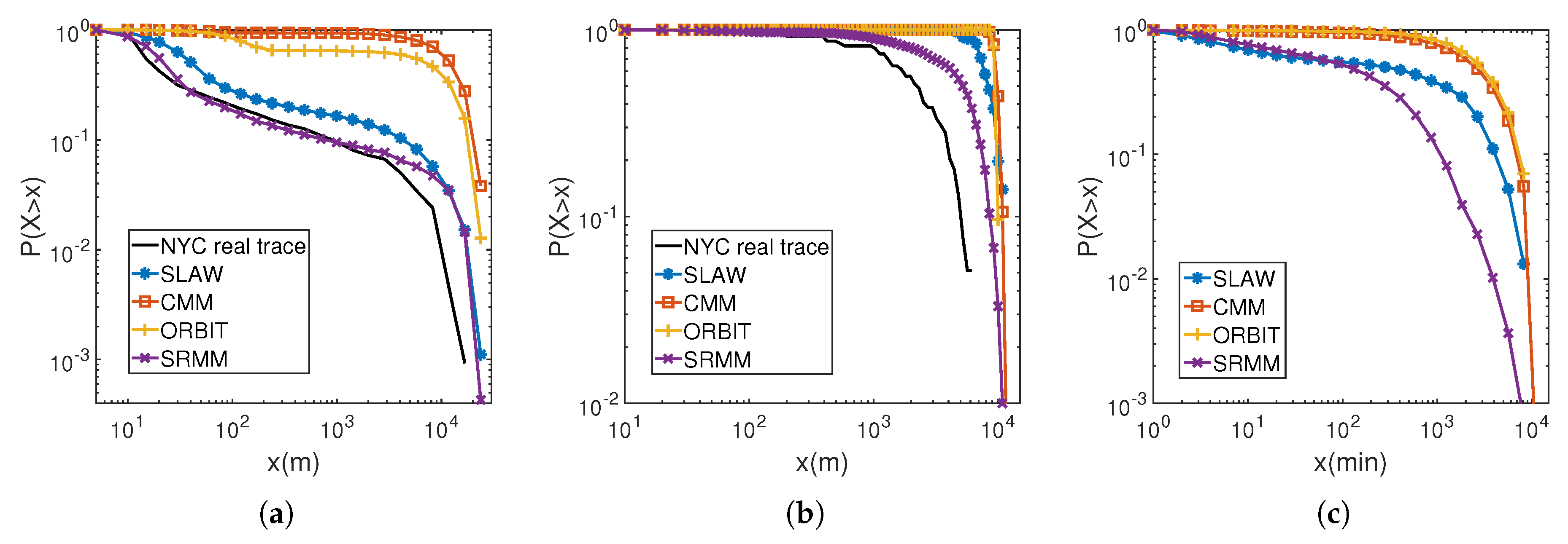
In SRMM, the pause-time distribution was already set to follow a truncated power-law distribution with a range of values from 0.5 to 700 min. Thus, this section verifies other human movement characteristics (i.e., the distributions of flights, the radii of gyration, and ICTs). First, KL divergence, K-S test, WMRD are used to validate our model with the real trace. Several studies analyzed real traces, and showed that the distributions of flights, radii of gyration, and ICTs in real traces follow truncated power-law distributions [3,4,9]. Therefore, AIC and BIC between a truncated power-law distribution and an exponential distribution over human characteristics are compared to show whether the human characteristics follow truncated power-law distributions or not.

Flight

We first consider the flight distribution with various parameter values for SRMM. Figure 5 shows KL divergence between the real trace flight distribution and the synthetic ones generated by SRMM using various parameter values. A lower value for KL divergence implies that generated flight lengths are a better fit to the real trace.

In Figure 5a, KL divergence with various values for $\alpha$ is presented. In general, KL divergence decreases when $\alpha$ increases from $0.8$ to $1.6$, and increases when $\alpha$ increases from $1.6$ to $2.0$. The values for KL divergence show that SRMM matches the real flight distribution well, especially when $\alpha$ is equal to $1.6$.

Figure 5b shows the effect of $\beta$ on KL divergence. Overall, the flight distributions are close to the real flight, and when $\beta =1.6$, the flight distribution is a better fit to the real flights than the others.

KL divergence with various values of $\rho$ is shown in Figure 5c. In general, KL divergence values decrease when $\rho$ increases from 0.4 to 0.8. When $\rho =0.8$, the flight distribution is the closest approximation to the real one. When $\rho =1$ (i.e., the social relationships between people are not considered), the KL divergence value is larger than KL divergence in case $\rho =0.8$. This indicates that to obtain flights that match the real flights well, the social relationship is important, and it should be considered.

Figure 5d displays the KL divergence values with various values of $\gamma$. As shown in the figure, we obtain the best result for KL divergence when $\gamma =0.8$.

In Figure 5e, KL divergence with various values of $\theta$ is presented. As shown in the results from KL divergence, all synthetic flights fit closely to the real one. when $\theta =0.8$, the flight distribution is a better fit to the real flights than the others.

Following results of KL divergence in Figure 5, the values of $\alpha ,\beta ,\rho ,\gamma ,$ and $\theta$ in SRMM are set to $1.6,1.6,0.8,0.8,$ and $0.8$, respectively.

Now, we verify our flight distribution with results from other models. The flight distributions obtained from various models are shown in Figure 6a, and the closeness of the flight distributions in synthetic models to real flights is shown by values in

Table 3. KL divergence, P value of K-S test, and WMRD between the real trace distributions (flight distribution and radius of gyration distribution) and the distributions generated by the synthetic models shown in Figure 6a,b.

	SRMM		SLAW		CMM		ORBIT
	Flight	Radius of Gyration	Flight	Radius of Gyration	Flight	Radius of Gyration	Flight	Radius of Gyration
KL divergence with real trace	0.0325	0.5211	0.0625	0.6627	0.3205	0.6921	0.2985	0.7223
WMRD	0.7716	1.9260	0.9868	1.9900	1.8420	2.0000	1.6658	2.0000
P value of K-S test	$1.01\times {10}^{-24}$	0.5180	$8.88\times {10}^{-119}$	$4.63\times {10}^{-16}$	0	$2.23\times {10}^{-24}$	0	$3.02\times {10}^{-26}$

. A model with a lower value for KL divergence and WMRD, and a higher value for P value of K-S test implies that the model is a better fit to the real trace. From the figure and the values shown in Table 3, it is clear that SRMM most closely matches the real flight distribution. For example, KL divergence with SRMM is 0.0325, whereas SLAW and CMM are 0.0625 and 0.3205, respectively. SRMM also obtained the lowest value for WMRD (i.e., 0.7716) and the highest value of P value of K-S test (i.e., $1.01\times {10}^{-24}$). The flight distribution with SLAW is also close to the real trace. In ORBIT and CMM, the spots were not generated by using fractal spots, and the distance was not considered when choosing the destinations. These are the main reasons for a large difference between these models and the real trace.

To check whether the generated flight distributions follow truncated power-law distributions,

Table 4. Results from AIC and BIC between a truncated power-law distribution (denoted as P$\mathrm{ow}$) and an exponential distribution (denoted as E$\mathrm{xp}$) over flights, the radius of gyration (denoted RoG), and ICT$\mathrm{s}$ of the New York City trace (denoted NYC) and various synthetic models with the synthetic map.

	SRMM			SLAW			CMM			ORBIT			NYC
	Flight	RoG	ICT	Flight	RoG	ICT	Flight	RoG	ICT	Flight	RoG	ICT	Flight	RoG	ICT
Selected model by AIC	Pow	Pow	Pow	Pow	Pow	Pow	Pow	Pow	Pow	Pow	Pow	Exp	Pow	Pow	N/A
Selected model by BIC	Pow	Pow	Pow	Pow	Pow	Pow	Pow	Pow	Pow	Pow	Pow	Exp	Pow	Pow	N/A

shows AIC and BIC results between a truncated power-law distribution and an exponential distribution. As shown in Table 4, the flight distribution generated by SRMM is closer to a truncated power-law distribution than to an exponential distribution. The results also indicate that flight distributions generated by other models approximate truncated power-law distributions.

The Radius of Gyration

To validate the real radius of gyration, Figure 6b shows the radius of gyration distributions for the various models, and Table 3 presents the KL divergence between the real radius of gyration distribution and distributions generated by the synthetic models. As shown in Figure 6b and Table 3, the radius of gyration distribution generated by SRMM is closest to the distribution extracted from the real trace. Specifically, the radius of gyration generated by SRMM obtains the lowest values for KL divergence (i.e., 0.5211) and WMRD (i.e., 1.9260), and the highest value of P value of K-S test (i.e., 0.5180).

Table 4 presents the results of AIC and BIC between a truncated power-law distribution and an exponential distribution over the radius of gyration of the New York City trace and various synthetic models. AIC and BIC results indicate that the radius of gyration produced by SRMM is closer to a truncated power-law distribution than an exponential distribution.

Inter-Contact Time

There is no available contact information in the real trace [11,19]; hence, only ICT distributions from synthetic models are shown in Figure 6c. The ICT distribution generated by SRMM is close to the ICT distribution of SLAW.

To validate the truncated power-law distribution, the distributions in Figure 6c are also verified with AIC and BIC. The results from AIC and BIC are provided in Table 4. As can be seen in the table, ICT distributions generated by SRMM, SLAW, and CMM fit better to power-law distributions, whereas the ICTs of ORBIT fit better to an exponential distribution. The ICTs of CMM are usually a very long time since people can move to any of the places without periodicity, so the chances of two people meeting again after the first encounter are much lower. In ORBIT, each person randomly chooses a list of places and then randomly picks a place in that list to visit. Thus, two people rarely encounter each other, and the ICTs of ORBIT are also very long times.

4.2.2. Verifying Social Relationships

In this section, we evaluate how well the mobility models reflect social relationships. First, we define the same social group ratio (SSGR), and we describe how to calculate this value. Then, the obtained results for the same social group ratio are presented.

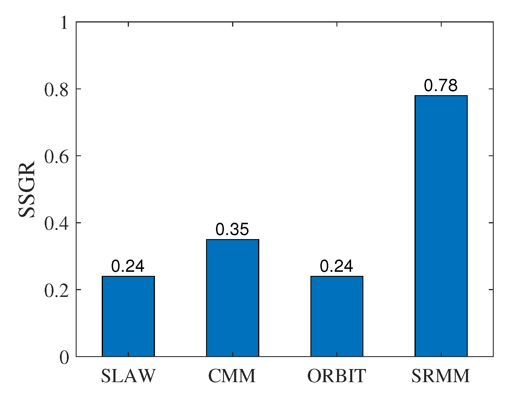
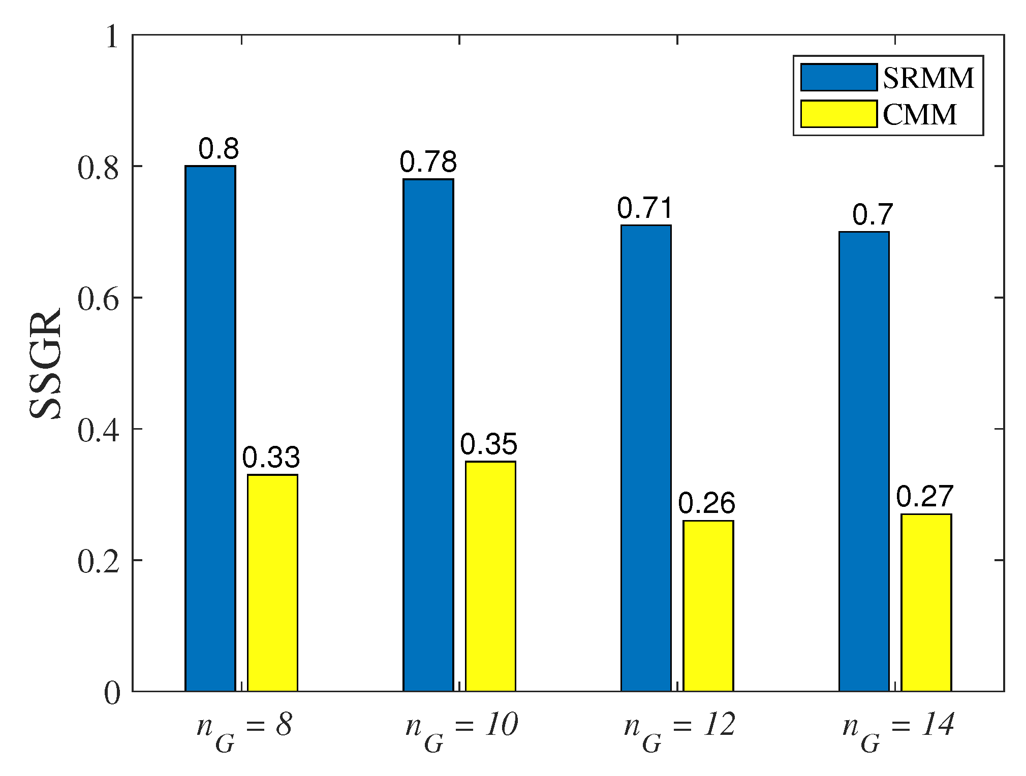
The Same Social Group Ratio

Mobility models and corresponding output mobility traces should reflect social relationships embedded in the input social graph. Please note that from a mobility trace of a mobility model, a social graph can also be obtained based on encounter rates between people (i.e., people, who have high encounter rates, will have strong relationships). A mobility model well reflects social relationships in the input social graph if the social graph obtained from the mobility trace of the model is similar to the input social graph. To determine the similarity between those two social graphs, social groups, which are obtained from those social graphs, are compared. People in a social group have strong social relationships. Therefore, if social groups in two social graphs are similar, two social graphs should be similar. To compare social groups in two social graphs, a new performance metric, called the same social group ratio (SSGR), is defined. Specifically, a set of social groups, ${\mathbb{S}}_G$, is obtained by using information from the input social graph. Based on the mobility trace generated by the mobility model, we also obtain a social graph and another set of social groups. Let this set be ${\mathbb{S}}_G^{syn}$. Then, for each group in ${\mathbb{S}}_G$, we select a corresponding group from ${\mathbb{S}}_G^{syn}$ to form a pair of groups. Please note that each group is only assigned to one pair, and pairs of groups are determined to maximize the number of common people in those pairs. The ratio of the total number of common people in all pairs to the total number of people in the network is defined as the same social group ratio. A high value for SSGR indicates that the mobility model highly reflects the social relationship. For example, ${\mathbb{S}}_G=\{G_1,G_2,G_3\}$. Group $G_1$ consists of $u_1$, $u_2$, and $u_3$; $u_4$ and $u_5$ belong to group $G_2$; group $G_3$ includes $u_6$ and $u_7$. For ${\mathbb{S}}_G^{syn}=\{G_1^{\prime },G_2^{\prime },G_3^{\prime }\}$; $u_1$, $u_2$, and $u_4$ belong to group $G_1^{\prime }$; group $G_2^{\prime }$ includes $u_3$ and $u_5$; group $G_3^{\prime }$ consists of $u_6$ and $u_7$. Based on maximizing the common people in pairs of groups, groups $(G_1,G_2,G_3)$ in ${\mathbb{S}}_G$ correspond to groups $(G_1^{\prime },G_2^{\prime },G_3^{\prime })$ in ${\mathbb{S}}_G^{syn}$, respectively. Specifically, the pair ($G_1,G_1^{\prime }$) has two common members, $u_1$ and $u_2$. The pair ($G_2,G_2^{\prime }$) has one common member, $u_5$, while $u_6$ and $u_7$ are two common members in the pair ($G_3,G_3^{\prime }$). The total for the common members is 5. We obtain SSGR $=0.83$.

To calculate SSGR values for synthetic models, we performed the following process.

• First, we find the social group set, ${\mathbb{S}}_G$. Set ${\mathbb{S}}_G$ is extracted from the social matrix during phase 1 in SRMM. For a fair comparison in SRMM, SLAW, CMM, and ORBIT, the same social group set is used.
• Secondly, to determine set ${\mathbb{S}}_G^{syn}$, we analyze the synthetic trace of each model to obtain a matrix of encounter rates ($ER$). The values in the $ER$ matrix are the number of times people encounter each other over the total simulation time. Suppose m and n denote two arbitrary people. $E_{m,n}$ denotes the number of encounters between m and n during simulation time T. Let $b_{ER}(m,n)$ be the encounter rate between m and n. Then, $b_{ER}(m,n)$ is calculated as:

  $$\begin{array}{c}\hfill b_{ER}(m,n)={\displaystyle \frac{E_{m,n}}{T}}\end{array}$$

  (12)
  In reality, people who have strong relationships tend to meet each other frequently [36,37]. Thus, a higher value in the $ER$ matrix can represent a stronger relationship between people. Then, the $ER$ matrix is used by the spectral clustering algorithm to obtain social group set ${\mathbb{S}}_G^{syn}$. The values in the $ER$ matrix are normalized to within the range [0,1] before the matrix is used in spectral clustering.
• Finally, we compare ${\mathbb{S}}_G$ and ${\mathbb{S}}_G^{syn}$ to obtain the SSGR value.

The Results of the Same Social Group Ratio

SSGR values from various models are shown in Figure 7. As can be seen in the figure, the results obtained from CMM and SRMM are higher than from SLAW and ORBIT because only CMM and SRMM consider social relationships between people. SRMM takes into account many social contexts, whereas CMM considers only a few, which leads to the higher SSGR with SRMM. Specifically, in CMM model, the destination can be selected from all places in the network. There are no set of frequently visited places for the people in a social group and no set of candidate places as in our model. Therefore, people in a social group have a low possibility to encounter in a wide area. That leads to a lower value of SSGR.

Because the number of social groups ($n_G$) in the area is not considered in SLAW and ORBIT, that does not affect human movements in that models. Therefore, Figure 8 only displays SSGR with different $n_G$ values in CMM and SRMM. In general, SSGR values decrease when $n_G$ increases. People in CMM may visit different places in the network, so increasing $n_G$ leads to a significant decrease in the probability that people will visit the places their social friends are visiting. Therefore, when $n_G$ is a higher value, SSGR from CMM is lower and close to the SSGR values from ORBIT and SLAW. In contrast, in SRMM, people in the same social group have the same frequently visited places and usually encounter each other. Thus, we still obtain a high value of SSGR from SRMM.

4.3. Real Road Map

In this section, to obtain more realistic human movements, the mobility models are considered on the real road map. For generating spots on the map, the bursty spot model is also used. First, spots are normally generated, and then spots are mapped to the nearest point on the nearest road on the map.

In this simulation, we use the real road map of Helsinki downtown [12]. The size of this map is 8.3 km × 7.31 km and the number of generated spots, $n_s$, is set to 978. Figure 9 shows generated spots on the real road map of Helsinki downtown.

In the mobility models, to move between two spots on the real road map, the shortest path between two spots is used. This path is obtained by using Dijkstra’s algorithm [38].

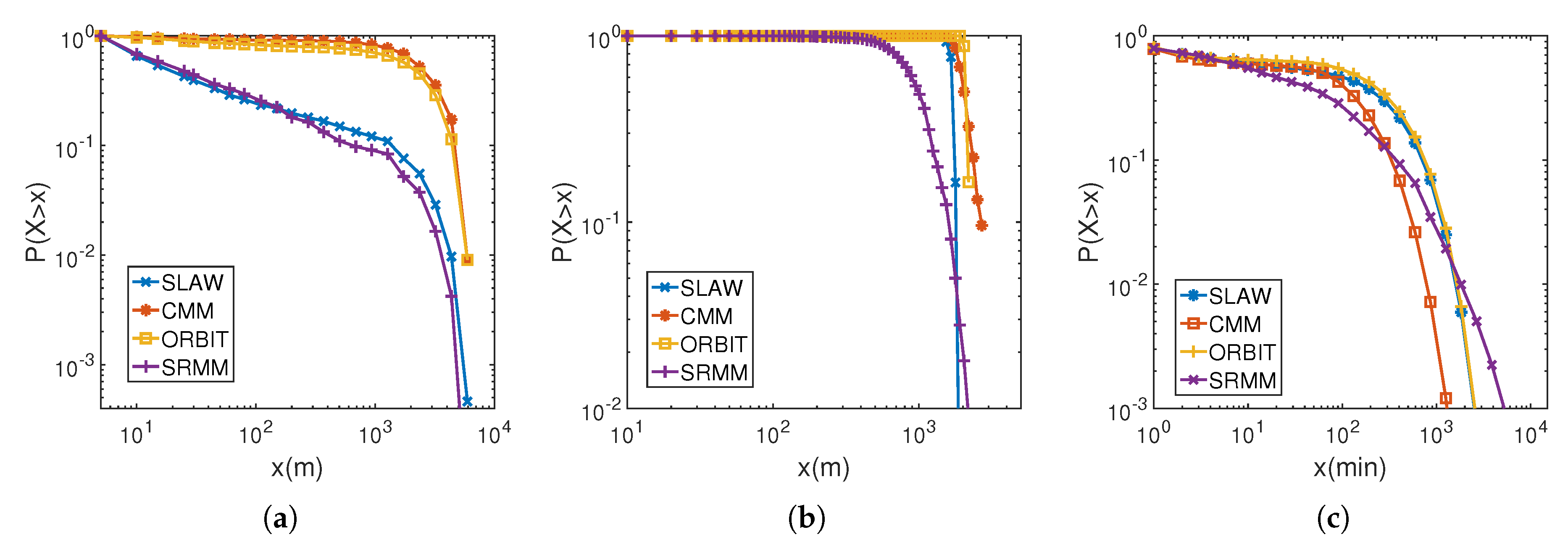
4.3.1. Verifying the Human Movement Characteristics

In this section, the distributions of flights, ICTs, and the radius of gyration are presented. AIC and BIC criteria are also used to verify that flights, inter-contact time, and the radius of gyration follow truncated power-law distributions. There are no available real mobility traces on the real road map of Helsinki downtown. Therefore, the KL divergence for comparing the synthetic models with real traces is not collected.

Flight

To validate the flight distribution, Figure 10a presents flight distributions from various models on the real road map. As can be seen in the figure, most of the flights from CMM and ORBIT are long flights. Flights generated by SRMM and SLAW are similar and more natural than the flights from CMM and ORBIT.

Table 5. Results from AIC and BIC between a truncated power-law distribution (denoted as P$\mathrm{ow}$) and an exponential distribution (denoted as E$\mathrm{xp}$) over flights, the radius of gyration (denoted RoG), and ICT$\mathrm{s}$ of various synthetic models with the real road map of Helsinki downtown.

	SRMM			SLAW			CMM			ORBIT
	Flight	RoG	ICT	Flight	RoG	ICT	Flight	RoG	ICT	Flight	RoG	ICT
Selected model by AIC	Pow	Pow	Pow	Pow	Pow	Pow	Pow	Pow	Pow	Exp	Pow	Pow
Selected model by BIC	Pow	Pow	Pow	Pow	Pow	Pow	Pow	Pow	Pow	Exp	Pow	Pow

shows AIC and BIC results between a truncated power-law distribution and an exponential distribution. From the figure and the values shown in Table 5, it is clear that the flight distributions from SRMM, SLAW, and CMM fit better to power-law distributions, whereas the flights of ORBIT fits better to an exponential distribution.

The Radius of Gyration

To check whether the generated radius of gyration distributions follow a truncated power-law distribution, the radius of gyration distributions from various models are shown in Figure 10b and Table 5 presents the results of AIC and BIC between a truncated power-law distribution and an exponential distribution over the radius of gyration. As shown in Figure 10b, the radius of gyration from SRMM is lower than those from other models. AIC and BIC results indicate that the radius of gyration generated by SRMM and all other models are closer to truncated power-law distributions than exponential distributions.

Inter-Contact Time

Figure 10c shows the ICT distributions from various mobility models. As shown in the figure, ICTs generated by SRMM are shorter than ICTs from other models since in our model, people in the same social group tend to frequently meet. Please note that the results of AIC and BIC are provided in Table 5. AIC and BIC results indicate that ICT distributions generated by SRMM, SLAW, CMM, and ORBIT fit better to power-law distributions than exponential distributions.

4.3.2. Verifying Social Relationships

In this subsection, the same social group ratio is obtained to verify that the mobility model can embody social relationships. Figure 11 presents SSGR values from various models. As can be seen in the figure, SSGR from CMM is slightly higher than from SLAW and ORBIT. The best result of SSGR is obtained from SRMM (i.e., 0.78), which indicates that social contexts between people are well embedded into our mobility model.

5. Conclusions

In this work, we proposed a novel human mobility model to address the limitations of existing human mobility models. Our proposed model takes into account the characteristics of human movement and the social context in human movement. Specifically, SRMM captures flights, the radius of gyration, ICTs, and pause times for realistic human movement. Then, many real contexts are considered in our model. For example, people prefer visiting nearby locations and are attracted to popular places. In the same social group, people usually tend to visit each other, and have the same frequently visited places. By reproducing real contexts, SRMM reflects social relationships in human movement.

To validate human movement characteristics, SRMM is considered on the synthetic map and the real road map. The results were compared with real human movements in a New York City trace and in other models (SLAW, CMM, and ORBIT). At first, KL divergence was used to show how well models match real traces. Then, AIC and BIC were used to evaluate the fit with truncated power-law distributions of human movement characteristics. Finally, we defined the same social group ratio to validate the reflection of social relationships in human mobility models.

The experiment results indicate that human movements from SRMM are more closely approximate real human movement characteristics, and clearly reflect the social relationships among people when we compare with other models. In future work, to make social contexts in the mobility model more realistic, we plan to use social graphs, in which a person can belong to multiple social groups.

References

1. Hyytia, E.; Lassila, P.; Virtamo, J. A markovian waypoint mobility model with application to hotspot modeling. In Proceedings of the IEEE International Conference on Communications, 2006, ICC’06, Istanbul, Turkey, 11–15 June 2006; Volume 3, pp. 979–986. [Google Scholar]
2. Royer, E.M.; Melliar-Smith, P.M.; Moser, L.E. An analysis of the optimum node density for ad hoc mobile networks. In Proceedings of the ICC 2001. IEEE International Conference on Communications. Conference Record (Cat. No.01CH37240), Helsinki, Finland, 11–14 June 2001; Volume 3, pp. 857–861. [Google Scholar]
3. Gonzalez, M.C.; Hidalgo, C.A.; Barabasi, A.L. Understanding individual human mobility patterns. Nature 2008, 453, 779–782. [Google Scholar] [CrossRef]
4. Rhee, I.; Shin, M.; Hong, S.; Lee, K.; Kim, S.J.; Chong, S. On the Levy-Walk Nature of Human Mobility. IEEE/ACM Trans. Netw. 2011, 19, 630–643. [Google Scholar] [CrossRef]
5. Lee, K.; Hong, S.; Kim, S.J.; Rhee, I.; Chong, S. SLAW: A New Mobility Model for Human Walks. In Proceedings of the IEEE INFOCOM 2009, Rio de Janeiro, Brazil, 19–25 April 2009; pp. 855–863. [Google Scholar]
6. Ekman, F.; Keränen, A.; Karvo, J.; Ott, J. Working Day Movement Model. In Proceedings of the 1st ACM SIGMOBILE Workshop on Mobility Models; ACM: New York, NY, USA, 2008; MobilityModels ’08; pp. 33–40. [Google Scholar]
7. Musolesi, M.; Mascolo, C. Designing Mobility Models Based on Social Network Theory. SIGMOBILE Mob. Comput. Commun. Rev. 2007, 11, 59–70. [Google Scholar] [CrossRef]
8. Boldrini, C.; Passarella, A. HCMM: Modelling spatial and temporal properties of human mobility driven by users’ social relationships. Comput. Commun. 2010, 33, 1056–1074. [Google Scholar] [CrossRef]
9. Chaintreau, A.; Hui, P.; Crowcroft, J.; Diot, C.; Gass, R.; Scott, J. Impact of Human Mobility on Opportunistic Forwarding Algorithms. IEEE Trans. Mobile Comput. 2007, 6, 606–620. [Google Scholar] [CrossRef]
10. Kim, M.; Kotz, D.; Kim, S. Extracting a Mobility Model from Real User Traces. In Proceedings of the IEEE INFOCOM 2006. 25TH IEEE International Conference on Computer Communications, Barcelona, Spain, 23–29 April 2006; pp. 1–13. [Google Scholar]
11. Rhee, I.; Shin, M.; Hong, S.; Lee, K.; Kim, S.; Chong, S. CRAWDAD Dataset ncsu/mobilitymodels (v. 2009-07-23). 2009. Available online: http://crawdad.org/ncsu/mobilitymodels/20090723 (accessed on 27 January 2020).
12. Maanmittauslaitos. The National Land Survey of Finland Topographic Database 03/2019. 2019. Available online: https://www.maanmittauslaitos.fi (accessed on 27 January 2020).
13. Kullback, S.; Leibler, R.A. On information and sufficiency. Ann. Math. Stat. 1951, 22, 79–86. [Google Scholar] [CrossRef]
14. Massey, F.J., Jr. The Kolmogorov-Smirnov test for goodness of fit. J. Am. Stat. Assoc. 1951, 46, 68–78. [Google Scholar] [CrossRef]
15. Duffield, N.; Lund, C.; Thorup, M. Estimating flow distributions from sampled flow statistics. IEEE/ACM Trans. Netw. 2005, 13, 933–946. [Google Scholar] [CrossRef]
16. Burnham, K.P.; Anderson, D.R. Multimodel Inference: Understanding AIC and BIC in Model Selection. Sociol. Methods Res. 2004, 33, 261–304. [Google Scholar] [CrossRef]
17. MacKay, D.J. Information Theory, Inference and Learning Algorithms; Cambridge University Press: Cambridge, UK, 2003. [Google Scholar]
18. Pfanzagl, J. Parametric Statistical Theory; Walter de Gruyter: Berlin, Germany, 1994. [Google Scholar]
19. McNett, M.; Voelker, G.M. Access and Mobility of Wireless PDA Users. SIGMOBILE Mob. Comput. Commun. Rev. 2005, 9, 40–55. [Google Scholar] [CrossRef]
20. Scott, J.; Gass, R.; Crowcroft, J.; Hui, P.; Diot, C.; Chaintreau, A. CRAWDAD Dataset Cambridge/Haggle (v. 2009-05-29). 2009. Available online: https://crawdad.org/cambridge/haggle/20090529 (accessed on 27 January 2020).
21. Stopczynski, A.; Sekara, V.; Sapiezynski, P.; Cuttone, A.; Madsen, M.M.; Larsen, J.E.; Lehmann, S. Measuring large-scale social networks with high resolution. PLoS ONE 2014, 9, e95978. [Google Scholar] [CrossRef] [PubMed] [Green Version]
22. Munjal, A.; Camp, T.; Navidi, W.C. SMOOTH: A Simple Way to Model Human Mobility. In Proceedings of the 14th ACM International Conference on Modeling, Analysis and Simulation of Wireless and Mobile Systems; MSWiM ’11; Association for Computing Machinery: New York, NY, USA, 2011; pp. 351–360. [Google Scholar] [CrossRef]
23. Solmaz, G.; Akbaş, M.; Turgut, D. A Mobility Model of Theme Park Visitors. IEEE Trans. Mobile Comput. 2015, 14, 2406–2418. [Google Scholar] [CrossRef]
24. Kang, X.; Liu, L.; Ma, H.; Zhao, D. Urban context aware human mobility model based on temporal correlation. In Proceedings of the 2017 IEEE International Conference on Communications (ICC), Paris, France, 21–25 May 2017; pp. 1–6. [Google Scholar] [CrossRef]
25. Mei, A.; Stefa, J. SWIM: A Simple Model to Generate Small Mobile Worlds. In Proceedings of the IEEE INFOCOM 2009, Rio de Janeiro, Brazil, 19–25 April 2009; pp. 2106–2113. [Google Scholar]
26. Zheng, Q.; Hong, X.; Liu, J.; Cordes, D.; Huang, W. Agenda Driven Mobility Modelling. Int. J. Ad Hoc Ubiquitous Comput. 2010, 5, 22–36. [Google Scholar] [CrossRef] [Green Version]
27. US Department of Transportation. 2001 National Household Travel Survey. 2007. Available online: http://nhts.ornl.gov (accessed on 27 January 2020).
28. Ghosh, J.; Philip, S.J.; Qiao, C. Sociological orbit aware location approximation and routing (SOLAR) in MANET. Ad Hoc Netw. 2007, 5, 189–209. [Google Scholar] [CrossRef]
29. Borrel, V.; Legendre, F.; de Amorim, M.D.; Fdida, S. SIMPS: Using Sociology for Personal Mobility. IEEE/ACM Trans. Netw. 2009, 17, 831–842. [Google Scholar] [CrossRef] [Green Version]
30. Yang, S.; Yang, X.; Zhang, C.; Spyrou, E. Using social network theory for modeling human mobility. IEEE Netw. 2010, 24, 6–13. [Google Scholar] [CrossRef]
31. Von Luxburg, U. A Tutorial on Spectral Clustering. Stat. Comput. 2007, 17, 395–416. [Google Scholar] [CrossRef]
32. MacQueen, J. Some methods for classification and analysis of multivariate observations. In Proceedings of the Fifth Berkeley Symposium on Mathematical Statistics and Probability, Oakland, CA, USA, 21 June 1967; Volume 1, pp. 281–297. [Google Scholar]
33. Ng, A.Y.; Jordan, M.I.; Weiss, Y. On spectral clustering: Analysis and an algorithm. In Proceedings of the 14th International Conference on Neural Information Processing Systems, Vancouver, BC, Canada, 3–8 December 2001; pp. 849–856. [Google Scholar]
34. Lee, K.; Hong, S.; Kim, S.J.; Rhee, I.; Chong, S. Demystifying Levy Walk Patterns in Human Walks. NCSU, Technical Report. 2008. Available online: http://netsrv.csc.ncsu.edu/export/Demystifying_Levy_Walk_Patterns.pdf (accessed on 27 January 2020).
35. Bohannon, R.W.; Andrews, A.W. Normal walking speed: A descriptive meta-analysis. Physiotherapy 2011, 97, 182–189. [Google Scholar] [CrossRef] [PubMed]
36. Bulut, E.; Szymanski, B.K. Exploiting Friendship Relations for Efficient Routing in Mobile Social Networks. IEEE Trans. Parallel Distrib. Syst. 2012, 23, 2254–2265. [Google Scholar] [CrossRef]
37. Li, F.; Wu, J. LocalCom: A Community-based Epidemic Forwarding Scheme in Disruption-tolerant Networks. In Proceedings of the 2009 6th Annual IEEE Communications Society Conference on Sensor, Mesh and Ad Hoc Communications and Networks, Rome, Italy, 22–26 June 2009; pp. 1–9. [Google Scholar]
38. Dijkstra, E.W. A note on two problems in connexion with graphs. Numer. Math. 1959, 1, 269–271. [Google Scholar] [CrossRef] [Green Version]
Figure 1. The social graph.
Electronics 09 00221 g001
Figure 2. The social groups.
Electronics 09 00221 g002
Figure 3. The dispersions of spots on the map. (a) New York City real map. (b) The synthetic map generated by BSM.
Electronics 09 00221 g003
Figure 4. Candidate places ( S C P u = S F P u S R P u ) and candidate spots ( S C S u = S F S u S R S u ) for person u.
Electronics 09 00221 g004
Figure 5. KL divergence between the real trace flight distribution and the synthetic ones generated by SRMM using various values for the parameters. (a) Various α values ( β = 1.6 , ρ = 0.8 , γ = 0.8 , θ = 0.8 ). (b) Various β values ( α = 1.6 , ρ = 0.8 , γ = 0.8 , θ = 0.8 ). (c) Various ρ values ( α = 1.6 , β = 1.6 , γ = 0.8 , θ = 0.8 ). (d) Various γ values ( α = 1.6 , β = 1.6 , ρ = 0.8 , γ = 0.8 , θ = 0.8 ) . (e) Various θ values ( α = 1.6 , β = 1.6 , ρ = 0.8 , γ = 0.8 ) .
Electronics 09 00221 g005
Figure 6. (a) Flight distributions of various models with the synthetic map. (b) The radius of gyration distributions of various models with the synthetic map. (c) ICT distributions of various models with the synthetic map.
Electronics 09 00221 g006
Figure 7. The same social group ratio values from various models with the synthetic map.
Electronics 09 00221 g007
Figure 8. The same social group ratio values for SRMM and CMM from various n G values.
Electronics 09 00221 g008
Figure 9. Generated spots on the real road map of Helsinki downtown.
Electronics 09 00221 g009
Figure 10. (a) Flight distributions of various models with the real road map. (b) The radius of gyration distributions of various models with the real road map. (c) ICT distributions of various models with the real road map.
Electronics 09 00221 g010
Figure 11. The same social group ratio values from various models with the real road map.
Electronics 09 00221 g011