Abstract
As a new generation of power-by-wire actuators, electromechanical actuators are finding increasingly more applications in the aviation field. Aiming at the application problem of the fault diagnosis of the electromechanical actuator, an improved diagnosis reasoning algorithm based on a hybrid timed failure propagation graph (TFPG) model is proposed. On the basis of this hybrid TFPG model, the activation conditions of OR and causality among nodes are given. The relationship discrepancy node is transformed into a relationship node and discrepancy node, which unifies the model storage process. The backward and forward extension operations of hypothesis generation and updating are improved. In the backward expansion operation, the specific process of backward update from non-alarm nodes is given, and the judging logic of the branch of relationship nodes is added, which guarantees the unity of the algorithm framework and the accuracy of the time update. In the forward expansion operation, the update order is adjusted to ensure the accuracy of the node update for the case of multiple parents. A hybrid TFPG model of the electromechanical actuator is established in the general modeling environment (GME), and a systematic verification scheme with two simulation types is tested with the application of the P2020 reference design board (RDB) and VxWorks 653 system. The results show that the proposed algorithm can realize the fault diagnosis of the electromechanical actuator as well as fault propagation prediction.
1. Introduction
The actuator is the key component driving the deflection of the aircraft surface. To accomplish a flight mission, the actuator causes the surface to deflect according to the given command. The consequences of actuator failure range from the degradation of flight performance to destruction of the aircraft and the deaths of crew members. With the sudden appearance and swift advancement of more/all-electric-aircraft (MEA/AEA), a power-by-wire actuation system has become the main motivator of aviation progression [1]. As one of the typical actuators of the power-by-wire actuation system, the electromechanical actuator (EMA) is small in size, is lightweight, yields no oil pollution and offers high efficiency [2]. While several studies on the modeling and control of electromechanical actuators exists [3,4,5], few studies addressed fault propagation and diagnosis. The research in this field will provide fault diagnosis and prediction measures and result in the extensive utilization of EMAs on aircraft.
TFPG was first proposed by Misra at Vanderbilt University [6]. It is a system-level diagnosis model that combines the failure propagation path and causality relationship to model faults and locate the failure mode according to the degree of compliance with the hypothesis. Typically, the TFPG relies on a hierarchy of functionalities and the search process is restricted only to the part where faults occur; it can realize the fault diagnosis of a single fault and of multiple faults; the structural redundancy principle is used to identify false and miss alarms; when the model validity decreases, the search process becomes restrict to the part with high validity.
A corresponding diagnosis algorithm based on a triggered sensor event was developed to diagnose single and multiple faults in components and sensors. Strasser et al. [7] provided a real-time incremental reasoning method that can deal with a variety of faults, including sensor faults and alarms. Abdelwahed et al. [8] proposed a qualitative condition-based diagnosis method with a multimode TFPG model, also known as a hybrid failure propagation graph (HFPG). The HFPG supports AND and OR semantics and can be used to construct complex failure propagation cases. Abdelwahed et al. [9] proposed an online diagnosis method based on consistency, which can identify various forms of alarms. The algorithm consists of two main steps: the first one generates the most consistent initial state assignment with the current observable states, and the second generates all consistent hypothesis sets from the given initial state assignment. Mahadevan et al. [10] focused on the distributed reasoning method. The large complex system model is partitioned into the smaller subsystem. Local reasoners interact with information via global reasoning, and the consistency of diagnosis results is ensured. Ge et al. [11] considered the uncertainty of the failure propagation path and added the information of failure probability. The failure propagation process was constructed by the probability TFPG model, which provided a certain basis for system hazard analysis [11].
The above studies focus mainly on the TFPG model and diagnosis algorithm. In addition, a few studies have been conducted on some extension problems. Bozzano et al. [12] proposed several new features of TFPGs based on symbolic technology, explored some important reasoning tasks, and ensured the effectiveness of online reasoning. Abdelwahed et al. [13] solved the problem of model-based prediction, put forward the main factors affecting the system reliability under a given state, and developed an algorithm to measure the system reliability. Abdelwahed et al. [14] introduced the concept of diagnosability; here, the diagnosability index was defined, and an evaluating algorithm was presented. Bittne et al. [15] generated a TFPG model automatically from software, relieving the developer from the tedious and error-prone task of constructing TFPGs manually. Priesterjahn et al. [16] also described how to generate TFPG automatically. Oonk et al. [17] input alarm data from the monitoring network and combined the TFPG with a Bayesian network to determine the optimal maintenance strategy. Troiano et al. [18] proposed an extended TFPG model, realizing both fault isolation and fault resolution.
The TFPG has been applied in engineering practice owing to its simplicity and effectiveness. Dubey et al. [19] utilized the TFPG to monitor the real-time system. In a NASA report [20], the effectiveness of the TFPG in the Boeing fuel system was verified and tested under 215 failure scenarios. The TFPG was applied in a conceptual fuel system to solve the problem of single and multiple fault diagnoses [21]. Abdelwahed et al. [22] mentioned some practical factors that needed to be considered, such as intermittent faults, alarms, limited computing resources, model validation and so on. Bittner et al. [23] applied the TFPG to the Solar Orbiter (a solar probe jointly developed by ESA and NASA), showing the value of the TFPG in safety analysis, fault diagnosis and isolation, and repair. Troiano et al. [24] also applied the TFPG to satellite fault diagnosis, isolation and repair. Xie et al. [25] designed a fault diagnosis framework for a test software based on TFPG. The simulation results showed that the diagnosis algorithm could diagnose a fault with time propagation characteristics.
The contributions of this brief are therefore as follows: As noted above, although the OR and AND discrepancy notes have been addressed in certain published works, the corresponding reasoning algorithm for applications has not been given. In this brief, a transformation technique is used, and the graph storage process is improved, which opens up the possibility to improve the node state updates in the faulty reasoning process. The proposed method cannot only detect various types of fault modes but also has a similar structure with the traditional fault tree analysis (FTA) method, which is conducive to the application of the proposed method in practical systems. On the basis of the proposed improved reasoning algorithm, an example fault diagnosis of an electromechanical actuator is presented. The failure modes can be located, and a fault forecast can be offered to some extent.
The paper is organized as follows: Section 2 presents the basic knowledge of the TFPG model, and the storage of the hybrid TFPG model is improved. A fault diagnosis algorithm based on a hybrid TFPG, which involves hypothesis initialization, hypothesis updating and hypothesis measure, is discussed in Section 3, and three subalgorithms are given. Case analysis simulation results are presented in Section 4. Finally, the conclusions of this paper are given in Section 5.
2. TFPG Model
This section mainly defines the TFPG model. Apart from the basic definition, two types of causality relationships are introduced, and on this basis, the improvements in the storage of the graph are presented.
2.1. Basic Knowledge of the TFPG Model
The occurrence of a fault will lead to one or more alarms in a system. Due to the dynamic characteristics of a system, fault propagation requires a certain period of time. Taking this time constraint when a fault occurs into consideration, the causality model describing the system behavior is the so-called TFPG model.
Definition 1.
A hybrid TFPG model can be presented by a tuple
whereis the set of failure mode nodes;is the set of discrepancy nodes, with;is the set of edges, with;represents a fixed time interval, and; anddefines the type of causal relationship between discrepancy nodes.
To facilitate the subsequent reasoning, the following assumptions are made:
- (1)
- The fault mode is the root node, which can be only the source node of the fault propagation path, but not the target node;
- (2)
- Self-circulation is not included;
- (3)
- Each node is connected to at least one fault propagation path;
- (4)
- The fault propagation path has no memory and will not fail.
The TFPG is a type of marked directed graph. The nodes in the graph represent the failure mode or fault discrepancy node, and the edges connecting nodes represent the transmission of a fault over time in the dynamic system, as described in Table 1.

Table 1.
Descriptions of the timed failure propagation graph (TFPG) element.
2.2. Causal Relationship
When the discrepancy node has more than one parent node, its activation is based on a certain causal relationship. The conditions for each causality relationship are different.
Definition 2.
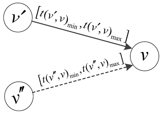
OR causal relationship: For any parent nodeof the discrepancy nodeshown in Figure 1, ifand the edgeis activated at time, theandsatisfy the OR causality with the following conditions at time:, where.
Figure 1.
Diagram of OR causality relationship.
Definition 3.
AND causal relationship: For any parent node of the discrepancy nodeshown in Figure 2, with,andsatisfy the AND causality with the following conditions at time:
- , whereis activated at time;
- , that is, when any parent nodeof the discrepancy nodeis activated, the edgeis also activated.

Figure 2.
Diagram of AND causality relationship.
2.3. Storage of the Hybrid TFPG Model
A hybrid TFPG is represented by a graph . Suppose there are failure mode nodes and discrepancy nodes exist in the graph . The relationship discrepancy node is transformed into a relationship node and a common discrepancy node, as shown in Figure 3 and Figure 4. The relationship node and the discrepancy node are connected by an edge, and the activation time interval of the edge is zero. In researching the reasoning algorithm, we need to consider only the influence of the AND causality. Suppose AND discrepancy nodes exist, and each discrepancy node is expressed as , in which the former nodes are the ordinary discrepancy node, and the latter nodes are the transformed relationship node.
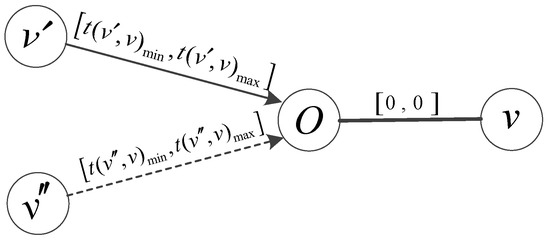
Figure 3.
Transformation of the OR discrepancy node.
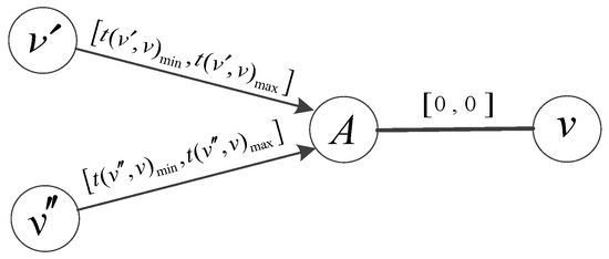
Figure 4.
Transformation of the AND discrepancy node.
When the failure mode node and the discrepancy node are not distinguished, the node is represented as , where the number of failure mode node ranges from 1 to , and the number of discrepancy nodes is from to .
Remark 1.
The above numbering rule is designed to help unify the reasoning framework and make its realization easier through computer programming.
According to the TFPG model, the adjacency matrix and reachability matrix can be obtained. is the adjacency matrix of the dimensions generated by graph . If , that is, a connection exists between and , then ; otherwise . represents the transitive closure of , if a path from to exists, then ; otherwise, .
and represent the minimum reachable time matrix and the maximum reachable time matrix, respectively.
3. Fault Diagnosis Algorithm Based on Hybrid TFPG
Fault diagnosis based on the hybrid TFPG is first triggered by the alarm event sent by the sensor, where is the discrepancy node of the activated alarm and is the time at which the signal is observed. When the state of the discrepancy node changes, a valid hypothesis of the current system is generated or updated according to the causality and time consistency of the discrepancy node. Finally, a set of hypotheses is selected as the most reasonable estimation of the current system state according to the measurement result. The specific process is shown in Figure 5.
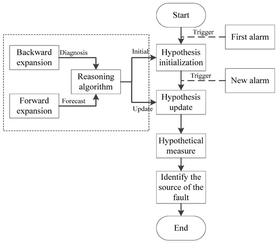
Figure 5.
Fault diagnosis process based on TFPG.
3.1. Hypothesis Initialization
The hypothesis initialization involves estimating the state of each node in the hybrid TFPG model and the time interval in which the node state changes based on the observed alarms.
Definition 4.
The hypothesis of failure modeis expressed as
whereis the failure mode supported by the hypothesis;is the estimation of the earliest time of each node state change in the TFPG model;is the estimation of the latest time of each node state change;represents the set of alarm nodes that support the hypothesis;refers to the set of alarm nodes that should not have occurred, but did occur under the hypothesis;refers to the set of alarm nodes that should have occurred, but did not occur under the hypothesis, andrepresents the set of alarm nodes that support the hypothesis, but have not been triggered under the current hypothesis.
The purpose of hypothesis initialization is to generate a new hypothesis when the system receives the first alarm. The node with the first alarm is selected as the initial state allocation node to find the fault mode supporting the alarm. The specific algorithm is as follows:
| Algorithm 1. Hypothesis initialization algorithm based on alarm triggering. |
|
3.1.1. Algorithm 2: Backward Extension Algorithm
| Algorithm 2. |
|
Remark 2.
Step 2.3 is the branch of the AND relationship node. As analyzed inSection 2.2, if any one of the parents of the OR discrepancy node is active, the link between them is enabled, and the time it takes for propagation is consistent with the hypothesis, then the OR discrepancy node is enabled. Thus, the OR relationship node can be dealt with as a common discrepancy node.
3.1.2. Algorithm 3: Forward Expansion Algorithm
| Algorithm 3. |
|
Remark 3.
Because the alarm has not reached the child node, the alarm clock is not offered. When updating the enabled time range of the child node, the early time and the late time are used.
3.1.3. Algorithm 4: Search Algorithm for Missing Alarm Nodes
| Algorithm 4. |
|
3.2. Hypothesis Updating
When a new alarm arrives, the existing hypothesis needs to be re-evaluated and updated. The specific algorithm is as follows:
| Algorithm 5.Hypothesis updating algorithm based on new alarm triggering. |
|
3.3. Hypothesis Ranking
When a TFPG fault diagnosis report contains multiple hypotheses, use the following two metrics to evaluate which hypothesis is the best explanation for the current fault.
Plausibility: the ratio of the number of alarms supporting this hypothesis to the total number of alarms. When neither or exists, all triggered alarms are support alarms, and the confidence level is 1.
Robustness: the ratio of the number of triggered alarms contained in the fault feature to the total number of expected alarms (if the fault hypothesis is correct). It is used to measure the extent to which the current hypothesis remains unchanged, and it can help in determining when to take action to repair the system.
4. Case Analysis
4.1. Working Principle of the Electromechanical Actuator
The electromechanical actuator is mainly composed of an electric control unit, the brushless DC motor, a mechanical ratio changer and an angle sensor. Its structure diagram is shown in Figure 6. The command signal is issued, and after modulation and power amplification, the motor rotates. The mechanical ratio changer then takes a high-speed, low-torque rotation from the electric motor and provides a lower-speed, higher-torque motion to the surface. Finally, the sensor on the surface gives feedback to the control unit, and thus a closed-loop control is formed.
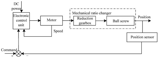
Figure 6.
Structural diagram of the electromechanical actuator.
4.2. EMA Hybrid TFPG Model
Figure 7 displays the TFPG model of the electromechanical actuator, and the description of each node is given in Table A1 (Appendix A).
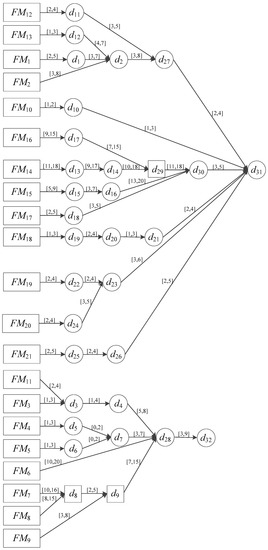
Figure 7.
TFPG model of the electromechanical actuator.
4.3. GME Modeling
To describe the TFPG model graphically, the GME is introduced, and the corresponding attributes for diagnosis and reasoning are integrated. The GME is a general and configurable modeling environment developed by the Vanderbilt University Institute for Software Integrated Systems that is mainly used for domain-specific modeling.
The main purpose of using the GME in this paper is to complete the meta modeling of the TFPG (to specify the modeling paradigm), that is, to configure and establish the basic elements (failure mode node, discrepancy node and fault propagation path) that meet the requirements of the TFPG, such as the attributes of discrepancy node and its connection with other nodes. The established metamodel of an EMA in the GME is shown in Figure A1. The TFPG model of EMA in GME is shown in Figure A2, Figure A3, Figure A4 and Figure A5. The TFPG model in the GME can clearly and accurately express the relationship between fault and alarm and the fault propagation time.
4.4. Simulation
In order to verify the effectiveness of the proposed method, we present a systematic verification scheme, as shown in Figure 8. The scheme mainly includes two parts: one is a digital simulation based on Matlab/Simulink, which mainly verifies the effectiveness of the proposed method; the other is real-time simulation, which mainly verifies the real-time performance of the proposed method. After the completion of the digital simulation, we use the Builder Object Network 2 (BON2) module of GME to generate the TFPG model. At the same time, we transform the fault diagnosis algorithm into C code, integrate the model and algorithm into P2020TDB, and conduct real-time simulation verification through the VxWorks 653 system.
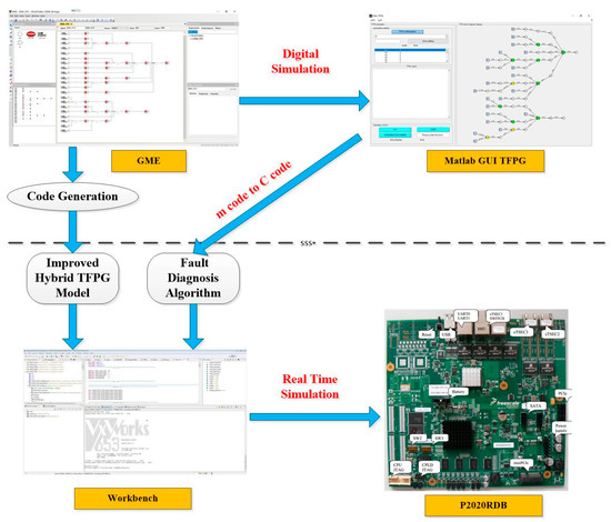
Figure 8.
The systematic verification scheme.
4.4.1. Digital Simulation
The hybrid TFPG model of an EMA is built in the GME. An XML file of the model is imported into Matlab GUI diagnostic software, and the diagnostic reasoning process is realized and verified.
Suppose alarms corresponding to occur at , at , at , at , at , at , at . The simulation time is set to 55. The red nodes in Figure 9 represent the alarm nodes. The simulation results are presented in Table 2.
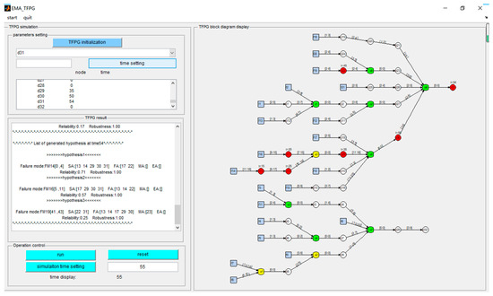
Figure 9.
Simulation settings.
Table 2.
Simulation results based on the improved method.
By analyzing the above simulation results, we can see the following:
- (1)
- When , an alarm occurs at , which produces Hypothesis 1. Potentially, will occur at and will alarm.
- (2)
- gives an alarm when . Since the alarm cannot be explained by Hypothesis 1, Hypothesis 2 is generated and is added to the FA set of Hypothesis 1.
- (3)
- triggers an alarm at , and Hypothesis 3 is added.
- (4)
- gives an alarm when . For Hypothesis 3, the alarm for is missing.
- (5)
- Finally, the reliability of Hypothesis 1 is found to be higher than that of other hypotheses and is considered to be the actual fault. As time passes, the credibility of Hypothesis 1 is assumed not to be 1, resulting from the false alarm and missed the alarm.
The innovation of this paper lies in the relationship discrepancy node is transformed into a relationship node, and the discrepancy node and the storage of the model are unified. In order to compare the effectiveness of the proposed method with that of the traditional TFPG method, a comparison with or without AND node is accomplished. The traditional TFPG method based simulation is shown in Table 3.
Table 3.
Table of simulation results based on traditional TFPG method.
It can be found that at the corresponding time, the traditional method will not generate a new fault mode () because the existing fault mode can explain the current alarm node. This method cannot only detect more fault modes but also has a similar structure to the traditional fault tree method, which is conducive to the application of this method in practical systems.
The analysis of the above results reveals that the improved hybrid TFPG reasoning algorithm can realize reasoning with relationship discrepancy nodes. It cannot only update the diagnosis results and locate the failure mode under normal alarm conditions but also identify false alarms and missing alarms with time.
4.4.2. Real-Time Simulation
In order to verify the real-time performance of the improved algorithm, a Freescale P2020RDB is applied, shown in Figure 10a, and the related instructions can be seen in [26]. The experimental platform is also built, and the connection between the P2020RDB and the computer is shown in Figure 10b. The configuration and programs are built on the computer and uploaded to the P2020RDB by Gigabit Ethernet. The configuration and improved algorithm of EMA is designed by VxWorks 653. Figure 11 shows the interface of VxWorks 653 and the basic configuration. The real-time monitoring results of EMA is shown in Figure 12. It can be seen that the improved algorithm can be conducted in the P2020RDB, and the result is the same as the digital simulation. The real-time performance of our algorithm is verified.
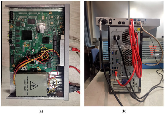
Figure 10.
(a) P2020RDB. (b) The connection of the platform.
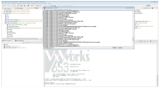
Figure 11.
The interface of VxWorks 653 and the basic configuration.
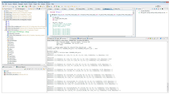
Figure 12.
The real-time monitoring results of electromechanical actuator (EMA).
5. Conclusions
In this paper, an improved hybrid TFPG model fault diagnosis reasoning algorithm is proposed and applied to the typical fault diagnosis of electromechanical actuators. Based on OR and AND discrepancy nodes, the activation conditions of the causality relationship are given. When the model is stored, the two relationship discrepancy nodes are transformed into relationship nodes and common discrepancy nodes, which is convenient for the unification of subsequent algorithms. Corresponding improvements to the updating of the AND relationship discrepancy nodes, the non-alarm parent nodes of alarm nodes and those nodes with multiple parent nodes in the extending backward and extending forward algorithm are achieved. Through the improved algorithm proposed in this brief, the failure mode can be located, and the purpose of fault diagnosis can be achieved.
6. Outlooks and Discussion
Although the fault diagnosis of EMA is realized in this paper, the algorithm still needs to be verified in practical application. In the future, the design and verification of an actual EMA fault diagnosis system should be applied by considering the aspects of fault signal measurement, fault information extraction, fault warning transmission, fault diagnosis, fault location and isolation. Therefore, the fault diagnosis algorithm should be able to locate the specific fault components faster and more accurately, which is our goal in further study.
Author Contributions
Y.C. conceived the presented idea. Y.C. and Y.L. developed the theory and performed the computations. Y.C. and Y.L. verified the analytical methods. X.W. supervised the findings of this work. All authors discussed the results and contributed to the final manuscript. All authors have read and agreed to the published version of the manuscript.
Funding
This work was supported by the National Natural Science Foundation of China (No. 61703341), Aeronautical Science Foundation of China (No. 20180753006), Natural Science Foundation of Shaanxi Province (2020JQ-218), the Fundamental Research Funds for the Central Universities (No. 3102019ZDHKY07) and Shaanxi Province Key Laboratory of Flight Control and Simulation Technology.
Acknowledgments
We thank Vanderbilt University for providing the fault modeling software GME. Thanks also to Ning Zhang and Chenxi Feng, who helped in the implementation of the TFPG algorithm.
Conflicts of Interest
The authors declare no conflict of interest.
Appendix A

Figure A1.
The metamodel of EMA in the general modeling environment (GME).

Figure A2.
The basic model of EMA in GME.

Figure A3.
The related submodel of EMA in GME.

Figure A4.
The alarm model of EMA in GME.

Figure A5.
The TFPG model of EMA in GME.
Table A1.
Descriptions of nodes in the TFPG model of the EMA.
Table A1.
Descriptions of nodes in the TFPG model of the EMA.
| Node | Description |
|---|---|
| Winding inter-turn short fault | |
| Winding phase-to-phase short fault | |
| Winding open fault | |
| Hall sensor open fault | |
| Hall sensor short fault | |
| Permanent magnet performance degradation | |
| Motor shaft crack | |
| Motor shaft wear | |
| Motor shaft deformation | |
| Motor shaft broken | |
| Inverter power tube open | |
| Inverter power tube short | |
| Inverter single bridge open | |
| Gear fatigue crack | |
| Gear broken | |
| Abnormal deceleration vibration of ball screw | |
| Screw channel blocked | |
| Sensor output oscillation | |
| Sensor output deviation | |
| Sensor output gained | |
| Sensor output fixed | |
| Temperature rise | |
| Winding overheat | |
| Current increasing | |
| Large motor speed and torque fluctuation | |
| Hall output high | |
| Hall output low | |
| Motor phase shortage | |
| Motor rotation noises | |
| Motor rotation vibration intense | |
| Motor failure | |
| Instant increase in short circuit current | |
| Non-fault phase currents increasing | |
| Crack propagation | |
| Gear noises increasing | |
| Gear slipping | |
| Bad gear meshing | |
| Screw noises increasing | |
| Ball screw blocked | |
| Surface output oscillation | |
| Motor reciprocating | |
| Mechanical ratio changer reciprocating | |
| Constant surface output deviation | |
| Control forced to correct errors | |
| Surface output scaled | |
| Surface output fixed | |
| Control error increasing | |
| Motor burn down | |
| Low motor efficiency | |
| Low deceleration efficiency | |
| Mechanical ratio changer failure | |
| Task failure | |
| Task affected |
References
- Huang, L.G.; Yu, T.; Jiao, Z.X.; Li, Y.P. Active Load-Sensitive Electro-Hydrostatic Actuator for More Electric Aircraft. Appl. Sci. 2020, 10, 6978. [Google Scholar] [CrossRef]
- Balaban, E.; Saxena, A.; Narasimhan, S.; Roychoudhury, I.; Koopmans, M.; Ott, C.; Goebel, K. Prognostic health management system development for electromechanical actuators. J. Aerosp. Inf. Syst. 2015, 12, 329–344. [Google Scholar] [CrossRef]
- Fu, J.; Maré, J.C.; Fu, Y.L. Modelling and simulation of flight control electromechanical actuators with special focus on model architecting, multidisciplinary effects and power flows. Chin. J. Aeronaut. 2017, 30, 47–65. [Google Scholar] [CrossRef]
- Merzouki, R.; Cadiou, J.C. Estimation of backlash phenomenon in the electromechanical actuator. Control Eng. Pract. 2005, 13, 973–983. [Google Scholar] [CrossRef]
- Qiao, G.; Liu, G.; Shi, Z. A review of electromechanical actuators for more/all electric aircraft systems. Proc. Inst. Mech. Eng. Part C J. Mech. Eng. Sci. 2017, 232, 4128–4151. [Google Scholar] [CrossRef]
- Misra, A. Sensor-Based Diagnosis of Dynamical Systems; Vanderbilt University: Nashville, TN, USA, 1994. [Google Scholar]
- Strasser, S.; Sheppard, J.W. Diagnostic Alarm Sequence Maturation in Timed Failure Propagation Graph; IEEE Autotestcon: Baltimore, MD, USA, 2011; pp. 158–165. [Google Scholar]
- Abdelwahed, S.; Karsai, G.; Biswas, G. System diagnosis using hybrid failure propagation graphs. In Proceedings of the 15th International Workshop Principles Diagnosis, Carcassonne, France, 23–25 June 2004. [Google Scholar]
- Abdelwahed, S.; Karsai, G.; Biswas, G. A consistency-based robust diagnosis approach for temporal causal systems. In Proceedings of the 16th International Workshop Principles Diagnosis, Pacific Grove, CA, USA, 1–3 June 2005; pp. 73–79. [Google Scholar]
- Mahadevan, N.; Abdelwahed, S.; Dubey, A. Distributed diagnosis of complex systems using timed failure propagation graph models. In Proceedings of the IEEE Systems Readiness Technology Conference, Orlando, FL, USA, 13–16 September 2010; pp. 124–129. [Google Scholar]
- Ge, X.Y.; Shen, G.H.; Huang, Z.Q.; Deng, L.M.; Wang, W.J. A hazard analysis method based on failure propagation model. Comput. Eng. Sci. 2019, 041, 1026–1033. [Google Scholar]
- Bozzano, M.; Cimatti, A.; Gario, M. SMT-based validation of timed failure propagation graphs. In Proceedings of the Twenty-Ninth Aaai Conference on Artificial Intelligence, Austin, TX, USA, 25–30 January 2015. [Google Scholar]
- Abdelwahed, S.; Karsai, G. Failure Prognosis Using Timed Failure Propagation Graphs. In Proceedings of the Annual Conference of the Prognostics and Health Management Society, San Diego, CA, USA, 27 September–1 October 2009. [Google Scholar]
- Abdelwahed, S.; Karsai, G. Notions of Diagnosability for Timed Failure Propagation Graphs; IEEE Autotestcon: Anaheim, CA, USA, 2006. [Google Scholar]
- Bittner, B.; Bozzano, M.; Cimatti, A. Automated synthesis of timed failure propagation graphs. In Proceedings of the International Joint Conference on Artificial Intelligence, New York, NY, USA, 9–15 July 2016. [Google Scholar]
- Priesterjahn, C.; Heinzemann, C.; Schafer, W. From timed automata to timed failure propagation graphs. In Proceedings of the IEEE International Symposium on Object/component/service-oriented Real-time Distributed Computing, Paderborn, Germany, 19–21 June 2013. [Google Scholar]
- Oonk, S.; Maldonado, F.J. Automated Maintenance Path Generation with Bayesian Networks, Influence Diagrams, and Timed Failure Propagation Graphs; IEEE Autotestcon: Anaheim, CA, USA, 2016. [Google Scholar]
- Troiano, L.; Cerbo, A.D.; Tipaldi, M. Fault detection and resolution based on extended time failure propagation graphs. In Proceedings of the International Conference on Soft Computing & Pattern Recognition, Fukuoka, Japan, 13–15 November 2015. [Google Scholar]
- Dubey, A.; Karsai, G.; Mahadevan, N. Model-based software health management for real-time systems. In Proceedings of the 2011 Aerospace Conference, Big Sky, MT, USA, 5–12 March 2011. [Google Scholar]
- Hayden, S.; Oza, N.; Mah, R. Diagnostic Technology Evaluation Report for on-Board Crew Launch Vehicle; NASA Technical Report; Ames Research Center: Moffett Field, CA, USA, 2006. [Google Scholar]
- Ofsthun, S.C.; Abdelwahed, S. Practical applications of timed failure propagation graphs for vehicle diagnosis. In Proceedings of the 2007 IEEE Autotestcon, Baltimore, MD, USA, 17–20 September 2007; pp. 250–259. [Google Scholar]
- Abdelwahed, S.; Karsai, G.; Mahadevan, N. Practical Implementation of Diagnosis Systems Using Timed Failure Propagation Graph Models. IEEE Trans. Instrum. Meas. 2009, 58, 240–247. [Google Scholar] [CrossRef]
- Bittner, B.; Bozzano, M.; Cimatti, A. Timed failure propagation analysis for spacecraft engineering: The ESA Solar Orbiter Case Study. In Proceedings of the International Symposium on Model-Based Safety and Assessment 2017, Trento, Italy, 11–13 September 2017; pp. 255–271. [Google Scholar]
- Troiano, L.; Tipaldi, M.; Di, C.A. Satellite FDIR practices using timed failure propagation graphs. In Proceedings of the 63rd International Astronautical Congress, Naples, Italy, 1–5 October 2012; pp. 8524–8531. [Google Scholar]
- Xie, W.Q.; Cai, Y.W.; Xing, X.C.; Xin, C.J. Algorithm design of failure diagnosis reasoned for software health management system. Meas. Control Technol. 2014, 33, 119–123. [Google Scholar]
- Conductor, Inc. Freescale Semiconductor Corp. In P2020 QorIQ Integrated Processor Reference Manual; Free-Scale Semiconductor: Austin, TX, USA, 2009. [Google Scholar]


Publisher’s Note: MDPI stays neutral with regard to jurisdictional claims in published maps and institutional affiliations. |
© 2020 by the authors. Licensee MDPI, Basel, Switzerland. This article is an open access article distributed under the terms and conditions of the Creative Commons Attribution (CC BY) license (http://creativecommons.org/licenses/by/4.0/).