Hyperspectral Image Denoising and Classification Using Multi-Scale Weighted EMAPs and Extreme Learning Machine

Abstract

Recently, extended multi-attribute profiles (EMAPs) have attracted much attention due to its good performance while applied to remote sensing images feature extraction and classification. Since the EMAPs connect multiple attribute features without considering the pixel-based Hyperspectral Image (HSI) classification, homogeneous regions may become unsmooth due to the noise to be introduced. To tackle this problem, we propose the weighted EMAPs (WEMAPs) to reduce the noise and smoothen the homogeneous regions based on weighted mean filter (WMF). Then, we construct multiscale WEMAPs to product multiscale feature in order to extract different spatial structures of the HSI and produce better classification results. Finally, a new joint decision fusion and feature fusion (JDFFF) framework is proposed based on the decision fusion (DF) and the multiscale WEMAPs (MWEMAPs) based on extreme learning machine (ELM) classifier. That is, the classification results from various scales are combined into a final one with ELM to perform the HSI classification. Experiment results show that the proposed algorithm significantly outperforms many state-of-the-art HSI classification algorithms.

1. Introduction

Hyperspectral images (HSIs) have been successfully applied in a wide range of applications, such as land and ocean mapping, geological analysis, brain cancer detection, mining, and precision agriculture [1,2,3]. As HSI contains rich spectral and spatial information, each pixel can be classified in the scene [4]. However, the supervised classification of the HSIs still remains a challenging task due to the unbalanced ratio between the limited training samples and the large number of spectral bands, i.e., the Hughes phenomenon [5]. To this end, many advanced techniques have been proposed for feature extraction and dimensionality reduction [6,7], such as the principal component analysis (PCA) and its variations [8,9], the attribute profiles (APs) [10,11], the linear discriminate analysis (LDA) [12], the nonparametric weighted feature extraction (NWFE) [13], and the singular spectrum analysis (SSA) [14], etc. In addition, a number of the state-of-the-art technologies have been successfully applied for HSI data classification, which include the support vector machine (SVM) [15], the extreme learning machine (ELM) [16], the sparse multinomial logistic regression (SMLR) and its variations [17,18], the active multi-kernel domain adaptation [1] and new parallel frameworks for auto-encoder training [19]. Among these approaches, the APs and the ELM have achieved much attention due to their good performances.

The APs were employed to extract the spatial information for remote sensing image classification, where the concepts have also been expanded to the morphological profiles (MPs) [20] and the extended morphological profiles (EMPs) [21]. The APs are found to be more useful in extracting spatial information than the MPs for the high resolution images [22]. As the original APs were extracted from each individual band, the dimensionality of the APs will become very high if all the spectral bands of the HSI were used [22]. To this end, the extended APs (EAPs) were introduced that only considered to extract APs from the first few principal components of the HSI [11]. By combining different EAPs, the extended multi-attribute profiles (EMAPs) were introduced [22], which can better model the spatial information of the HSI.

The APs and its variant EAPs have been widely applied for performing the HSI classification because of their good performance. For example, EAPs and the independent component analysis were combined for the classification of urban HSIs [23]. In [24], a generalized composite kernel based on EMAPs was proposed to extract both the spectral information and the spatial information for the HSI classification. In [22], EMAPs were combined with the random subspace for hyperspectral image classification. However, the APs and its variants, EAPs and EMAPs, still have some drawbacks, as explained below.

APs can be computed by several attributes, thickening and thinning operators, on an image with a group of thresholds. Consider two different cases: (1) Given a certain attribute such as an area, the AP of the area is determined by the given thresholds, yet the resulted structure varies according to the thresholds and spectral bands of the HSIs. (2) Different attributes may have various structural information. As the EMAPs were composed of EAPs with different attributes that consider the first several principal components of the HSIs, different attributes and thresholds may produce noise in the HSIs. Recently, the weighted mean filters (WMFs) [3] were found to be successful in reducing the noise and smoothening the homogeneous regions in HSIs. As a result, the WMF and the EMAPs are combined in our paper to form a new method namely the weighted EMAPs (WEMAPs) for effective denoising and feature extraction in HSIs.

For classification of HSIs, both decision-level fusion (DF) [3,25] and feature-level fusion (FF) [17,26] have been used. The FF aims to improve the discriminant ability by combining different features [26], where two features extracted by WEMAPs and WMFs are used. The DF such as the majority voting (MV) [27] is based on the probability output of each individual classifier to reach a joint decision [26]. In [28,29], DF and FF have been successfully combined for multimodal biometric authentication and emotion recognition. In [30], the combined DF and FF have been applied to the classification of both the HSIs and the LIDAR data. To the best of our knowledge, the work in [30] is the only reported one to use the DF and the FF simultaneously for HSI classification, by merely combining different MPs of the HSIs and the LIDAR. The HSIs may contain both small and large homogeneous regions due to their complex structures [3], yet the MPs may ignore the discriminative information of the HSIs [10]. In order to capture different spatial structures for more effectively modeling the discriminant information of the HSIs, a novel multiscale FF framework namely the joint FF and DF (JFFDF) based on both the WMF and the proposed WEMAPs is proposed in this paper for HSI classification.

Both the SVM and ELM have been widely used for HSI classification because of their abilities in handing the Hughes phenomenon [31]. However, it takes too much running time for SVM to solve a large constrained optimization problem [26]. Compared to SVM, the training for the ELM is simpler and faster [26] as the input weights and the bias between the input layer and the hidden layer of the ELM are randomly generated. Then, the classification results of various scales are combined into final one based on the proposed JDFFF. Details will be discussed in Section 3, including an overall flowchart in Figure 1. The main contributions of this work can be highlighted as follows: (1) The WEMAPs are proposed for integrating different EMAPs attributes to reduce the noise and smoothen the homogeneous regions. (2) The JDFFF framework is proposed to capture different spatial structures and better model the discriminant information of the HSIs. (3) The classification results of different scales are combined into a final one using the MV with the proposed JDFFF for the HSI classification.

The rest of this paper is organized as follows: Some related algorithms are reviewed in Section 2 and the proposed framework of the JDFFF is presented in Section 3; the extended experiment results and the analysis are presented in Section 4; Section 5 concludes our works with some remarks.

2. Introductions of Related Works

2.1. Normalization

As an important preprocessing step for HSI, there are a number of normalization approaches [26]. We chose the Max method for normalization for the purpose of simplicity and consistency since it is a widely used normalization method [26]. Given a HSI data $\mathrm{X}=\left[{\mathrm{x}}_1{}^{\ast },{\mathrm{x}}_2{}^{\ast },\dots ,{\mathrm{x}}_{\mathrm{N}}{}^{\ast }\right]\in {\mathrm{R}}^{\mathrm{d}\times \mathrm{N}}$, where N denotes the number of pixels in HSI and d is the number of bands of a HSI dataset. The Max normalization method can be expressed as:

$${\mathrm{x}}_{\mathrm{ij}}={\mathrm{x}}_{\mathrm{ij}}{}^{\ast }/\max \left(\mathrm{X}\right)$$

(1)

where $\max \left(\mathrm{X}\right)$ and ${\mathrm{x}}_{\mathrm{ij}}{}^{\ast }$ are the largest value of HSI and any pixel value of HSI, respectively.

2.2. Attribute Profiles (APs)

The mathematical morphology is a powerful framework for analyzing the spatial information of the HSIs [22,32,33]. Let ${\mathsf{\gamma }}_{\mathrm{R}}$ and ${\mathsf{\varphi }}_{\mathrm{R}}$ be the morphological opening and closing, and their operations on a grey level image $\mathrm{f}$ can be defined as [10]:

$${\mathsf{\gamma }}_{\mathrm{R}}^{\mathrm{i}}\left(\mathrm{f}\right)={\mathrm{R}}_{\mathrm{f}}^{\mathsf{\delta }}\left({\mathsf{\epsilon }}^{\mathrm{i}}\left(\mathrm{f}\right)\right)$$

(2)

$${\mathsf{\varphi }}_{\mathrm{R}}^{\mathrm{i}}\left(\mathrm{f}\right)={\mathrm{R}}_{\mathrm{f}}^{\mathsf{\epsilon }}\left({\mathsf{\delta }}^{\mathrm{i}}\left(\mathrm{f}\right)\right)$$

(3)

where ${\mathsf{\delta }}^{\mathrm{i}}$ and ${\mathsf{\epsilon }}^{\mathrm{i}}$ are the dilation and erosion with a given structure element of size i (i = 1, …, n), ${\mathrm{R}}_{\mathrm{f}}^{\mathsf{\delta }}$ and ${\mathrm{R}}_{\mathrm{f}}^{\mathsf{\epsilon }}$ are the geodesic reconstruction by the dilation and the erosion, respectively [32]. Then, the MPs can be defined as follows:

$$\mathrm{MPs}\left(\mathrm{f}\right)=\left\{{\mathsf{\gamma }}_{\mathrm{R}}^{\mathrm{n}}\left(\mathrm{f}\right),{ \mathsf{\gamma }}_{\mathrm{R}}^{\mathrm{n}-1}\left(\mathrm{f}\right),\dots ,{ \mathsf{\gamma }}_{\mathrm{R}}^1\left( \mathrm{f}\right), {\mathsf{\varphi }}_{\mathrm{R}}^1\left(\mathrm{f}\right),\dots , {\mathsf{\varphi }}_{\mathrm{R}}^{\mathrm{n}-1}\left(\mathrm{f}\right), {\mathsf{\varphi }}_{\mathrm{R}}^{\mathrm{n}}\left(\mathrm{f}\right)\right\}$$

(4)

Analogous to the MP, for a given sequence of thresholds ${\mathsf{\lambda }}_1, \dots ,{\mathsf{\lambda }}_{\mathrm{n}}$, the APs can be represented as a concatenation of a series of the attribute thinning and the attribute thickening operations [10,24] as follows:

$$\mathrm{APs}\left(\mathrm{f}\right)=\left\{{{\displaystyle \check{\mathsf{\gamma }}}}_{\mathrm{R}}^{\mathrm{n}}\left(\mathrm{f}\right), {\check{\mathsf{\gamma }}}_{\mathrm{R}}^{\mathrm{n}-1}\left(\mathrm{f}\right),\dots , {\check{\mathsf{\gamma }}}_{\mathrm{R}}^1\left(\mathrm{f}\right), \mathrm{f}, {\check{\mathsf{\varphi }}}_{\mathrm{R}}^1\left(\mathrm{f}\right),\dots , {\check{\mathsf{\varphi }}}_{\mathrm{R}}^{\mathrm{n}-1}\left(\mathrm{f}\right), {\check{\mathsf{\varphi }}}_{\mathrm{R}}^{\mathrm{n}}\left(\mathrm{f}\right)\right\}$$

(5)

where ${\check{\mathsf{\gamma }}}_{\mathrm{R}}$ and ${\check{\mathsf{\varphi }}}_{\mathrm{R}}$ denote the thinning and thickening transformations, respectively.

2.3. Extreme Learning Machine (ELM)

The ELM [34,35] was originally proposed for the single hidden layer feedforward neural network [36] with one linear output layer and one hidden layer [26]. Let $\mathrm{X}=\left[{\mathrm{x}}_1,{\mathrm{x}}_2,\dots ,{\mathrm{x}}_{\mathrm{n}}\right]\in {\mathrm{R}}^{\mathrm{d}\times \mathrm{n}}$ and $\mathrm{Y}=\left[{\mathrm{y}}_1,{ \mathrm{y}}_2,\dots ,{ \mathrm{y}}_{\mathrm{n}}\right]\in {\mathrm{R}}^{\mathrm{m}\times \mathrm{n}}$ be n training samples and their corresponding labels with $m$ classes, the output function of the ELM with L hidden neurons can be represented by:

$${\mathrm{f}}_{\mathrm{L}}\left({\mathrm{x}}_{\mathrm{i}}\right)={\sum }_{\mathrm{j}=1}^{\mathrm{L}}{\mathsf{\beta }}_{\mathrm{j}}\mathrm{h}({\mathrm{a}}_{\mathrm{j}},{\mathrm{b}}_{\mathrm{j}},{\mathrm{x}}_{\mathrm{i}})={\mathrm{y}}_{\mathrm{i}} \mathrm{for} \mathrm{i} = 1, \dots , \mathrm{n},$$

(6)

where ${\mathsf{\beta }}_{\mathrm{j}}$ is the output weight between the hidden layer and the output layer, $\mathrm{h}$, is the activation function. The above n equations can be rewritten in a matrix form as:

$$\mathrm{H}\mathsf{\beta }={\mathrm{Y}}^{\mathrm{T}},$$

(7)

where $\mathsf{\beta }={[{\mathsf{\beta }}_1, \dots ,{\mathsf{\beta }}_{\mathrm{L}}]}^{\mathrm{T}}\in {\mathrm{R}}^{\mathrm{L}\times \mathrm{m}}$ and

$$\mathrm{H}=\left[\begin{array}{ccc}\mathrm{h}\left({\mathrm{a}}_1,{\mathrm{b}}_1,{\mathrm{x}}_1\right)& \cdots & \mathrm{h}\left({\mathrm{a}}_{\mathrm{L}},{\mathrm{b}}_{\mathrm{L}},{\mathrm{x}}_1\right)\\ ⋮& \ddots & ⋮\\ \mathrm{h}\left({\mathrm{a}}_1,{\mathrm{b}}_1,{\mathrm{x}}_{\mathrm{n}}\right)& \cdots & \mathrm{h}\left({\mathrm{a}}_{\mathrm{L}},{\mathrm{b}}_{\mathrm{L}},{\mathrm{x}}_{\mathrm{n}}\right)\end{array}\right],$$

(8)

The solution of Equation (7) of the original ELM can be expressed by:

$$\mathsf{\beta }={\mathrm{H}}^{†}{\mathrm{Y}}^{\mathrm{T}},$$

(9)

where ${\mathrm{H}}^{†}$ is the Moore Penrose generalized inverse of the matrix $\mathrm{H}$ [37]. That is, ${\mathrm{H}}^{†}={\mathrm{H}}^{\mathrm{T}}{({\mathrm{HH}}^{\mathrm{T}})}^{-1}$ or ${\mathrm{H}}^{†}={({\mathrm{H}}^{\mathrm{T}}\mathrm{H})}^{-1}{\mathrm{H}}^{\mathrm{T}}$. A positive value $\frac{\mathrm{I}}{\mathrm{C}}$ is normally added to every diagonal element of ${\mathrm{HH}}^{\mathrm{T}}$ or ${\mathrm{H}}^{\mathrm{T}}\mathrm{H}$ in order to improve the stability and the generalization of the inverse operator [26], where $I$ is an identity mattrix. Finally, Equation (6) can be rewritten as:

$${\mathrm{f}}_{\mathrm{L}}\left({\mathrm{x}}_{\mathrm{i}}\right)=\mathrm{h}\left({\mathrm{x}}_{\mathrm{i}}\right)\mathsf{\beta }=\mathrm{h}\left({\mathrm{x}}_{\mathrm{i}}\right){({\mathrm{H}}^{\mathrm{T}}\mathrm{H}+\frac{\mathrm{I}}{\mathrm{C}})}^{-1}{\mathrm{H}}^{\mathrm{T}}{\mathrm{Y}}^{\mathrm{T}},$$

(10)

$$\mathrm{or}\hspace{1em}{\mathrm{f}}_{\mathrm{L}}\left({\mathrm{x}}_{\mathrm{i}}\right)=\mathrm{h}\left({\mathrm{x}}_{\mathrm{i}}\right)\mathsf{\beta }=\mathrm{h}\left({\mathrm{x}}_{\mathrm{i}}\right){\mathrm{H}}^{\mathrm{T}}{({\mathrm{HH}}^{\mathrm{T}}+\frac{\mathrm{I}}{\mathrm{C}})}^{-1}{\mathrm{Y}}^{\mathrm{T}},$$

(11)

It should be noted that the sizes of $\mathrm{I}$ in Equations (10) and (11) are different, which depend on the dimensions of ${\mathrm{H}}^{\mathrm{T}}\mathrm{H}$ and ${\mathrm{HH}}^{\mathrm{T}}$, respectively. Similar to the SVM [38,39], the output function of the ELM using the RBF kernel can be represented as follows:

$${\mathrm{f}}_{\mathrm{L}}\left({\mathrm{x}}_{\mathrm{i}}\right)=\mathrm{h}\left({\mathrm{x}}_{\mathrm{i}}\right)\mathsf{\beta }=\mathrm{h}\left({\mathrm{x}}_{\mathrm{i}}\right){\mathrm{H}}^{\mathrm{T}}{({\mathrm{HH}}^{\mathrm{T}}+\frac{\mathrm{I}}{\mathrm{C}})}^{-1}{\mathrm{Y}}^{\mathrm{T}}={\left[\begin{array}{c}\mathrm{K}\left({\mathrm{x}}_{\mathrm{i}},{\mathrm{x}}_1\right)\\ ⋮\\ \mathrm{K}\left({\mathrm{x}}_{\mathrm{i}},{\mathrm{x}}_{\mathrm{N}}\right)\end{array}\right]}^{\mathrm{T}}{({\mathsf{\Omega }}_{\mathrm{ELM}}+\frac{\mathrm{I}}{\mathrm{C}})}^{-1}{\mathrm{Y}}^{\mathrm{T}},$$

(12)

where ${\mathsf{\Omega }}_{\mathrm{ELM}}={\mathrm{HH}}^{\mathrm{T}},{ \mathrm{and} \mathsf{\Omega }}_{{\mathrm{ELM}}_{\mathrm{i},\mathrm{j}}}=\mathrm{h}\left({\mathrm{x}}_{\mathrm{i}}\right)\mathrm{h}\left({\mathrm{x}}_{\mathrm{j}}\right)=\mathrm{K}\left({\mathrm{x}}_{\mathrm{i}},{\mathrm{x}}_{\mathrm{j}}\right)$.

Two well-known constrained optimization models of the improved ELM are widely used. One is to define $\mathsf{\beta }$ in Equation (10) or Equation (11) without a kernel, which introduce a regularization term to ELM for overfitting problem called the generalized ELM (GELM) defined as follows:

$$\mathsf{\beta }=\mathrm{H}\ast (\frac{\mathrm{I}}{\mathrm{C}}+{\mathrm{H}}^{\mathrm{T}}\mathrm{H}{)}^{-1}{\mathrm{Y}}^{\mathrm{T}},$$

(13)

Another one is to introduce new kernels in Equation (12), which introduce the kernel function to GELM for kernel data representation called the kernel ELM (KELM) as defined below:

$$\mathsf{\beta }={(\frac{\mathrm{I}}{\mathrm{C}}+{\mathsf{\Omega }}_{\mathrm{ELM}})}^{-1}{\mathrm{Y}}^{\mathrm{T}}$$

(14)

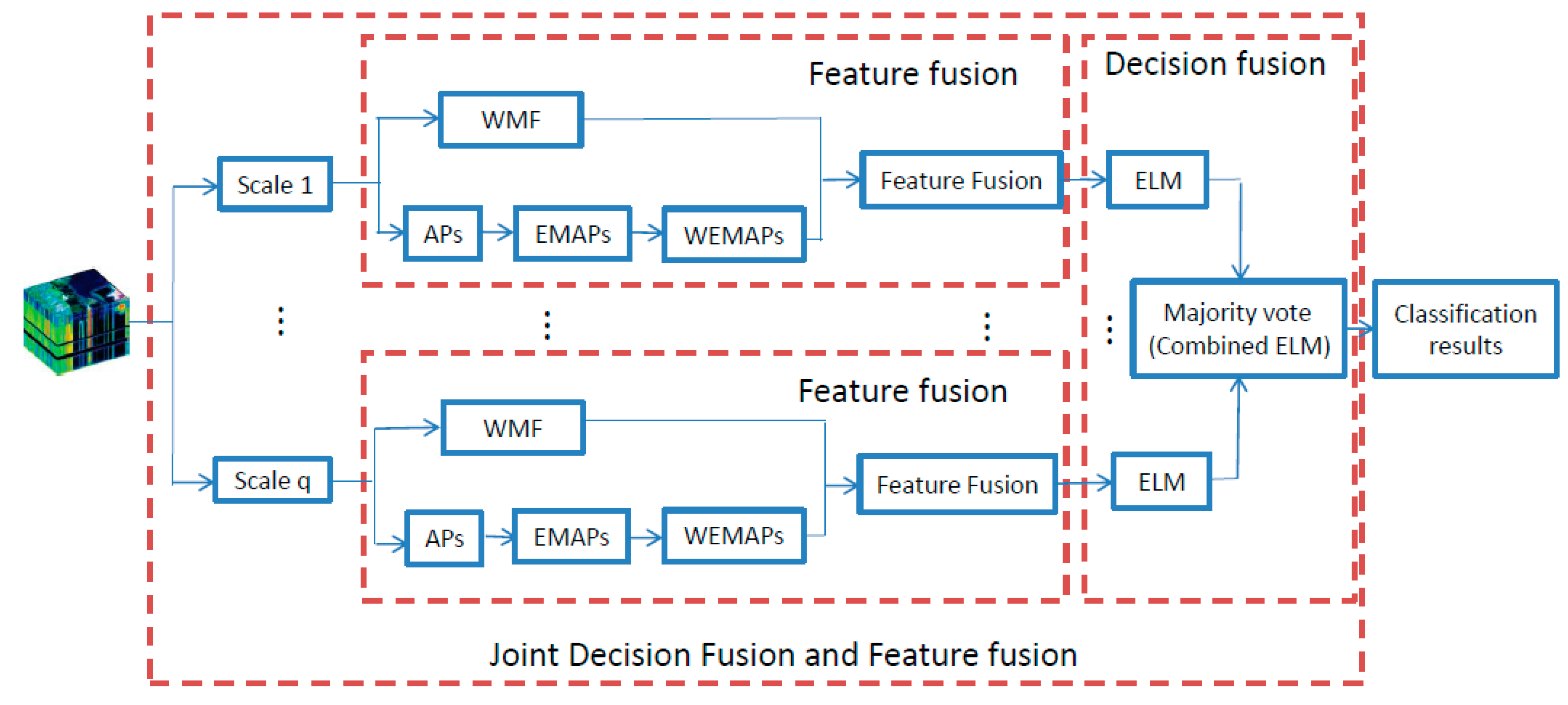
3. The Proposed Joint Decision Fusion and Feature Fusion (JDFFF) Framework

3.1. Weighted Mean Filters (WMFs)

For n training samples $\mathrm{X}=\left[{\mathrm{x}}_1,{\mathrm{x}}_2,\dots ,{\mathrm{x}}_{\mathrm{n}}\right]\in {\mathrm{R}}^{\mathrm{d}\times \mathrm{n}}$ and the corresponding class labels $\mathrm{Y}=\left[{\mathrm{y}}_1,{ \mathrm{y}}_2,\dots ,{ \mathrm{y}}_{\mathrm{n}}\right]\in {\mathrm{R}}^{\mathrm{m}\times \mathrm{n}}$, let $\left({\mathrm{p}}_{\mathrm{i}},{\mathrm{q}}_{\mathrm{i}}\right)$ be the spatial coordinate of the i-th training sample, ${\mathrm{x}}_{\mathrm{i}}$. The local pixel neighborhood centered at ${\mathrm{x}}_{\mathrm{i}}$ can be expressed by [3]:

$$\mathrm{N}\left({\mathrm{x}}_{\mathrm{i}}\right)=\{\mathrm{x}=\left(\mathrm{p},\mathrm{q}\right)|\mathrm{p}\in \left[{\mathrm{p}}_{\mathrm{i}}-\mathrm{c},{\mathrm{p}}_{\mathrm{i}}+\mathrm{c}\right],\mathrm{q}\in \left[{\mathrm{q}}_{\mathrm{i}}-\mathrm{c},{\mathrm{q}}_{\mathrm{i}}+\mathrm{c}\right]\},$$

(15)

where $\mathrm{c}=\frac{{\mathrm{w}}_0-1}{2}$, and $w_0$ is the odd width (scale) of the neighborhood window.

Let $\mathrm{s}=w_0{}^2-1$ denote the total number of the neighboring pixels of ${\mathrm{x}}_{\mathrm{i}}$, and also denote the pixels in its spatial neighborhood $\mathrm{N}\left({\mathrm{x}}_{\mathrm{i}}\right)$ by ${\mathrm{x}}_{\mathrm{i}}$, ${\mathrm{x}}_{\mathrm{i}1}$, ${\mathrm{x}}_{\mathrm{i}2}$, …, ${\mathrm{x}}_{\mathrm{is}}$. The spatial WMF of a labeled pixel ${\mathrm{x}}_{\mathrm{i}}$ can be represented by:

$${\mathrm{x}}_{\mathrm{i}}^{\mathrm{WMF}}=\frac{{\sum }_{{\mathrm{x}}_{\mathrm{j}}\in \mathrm{N}\left({\mathrm{x}}_{\mathrm{i}}\right)}{\mathrm{v}}_{\mathrm{j}}{\mathrm{x}}_{\mathrm{j}}}{{\sum }_{{\mathrm{x}}_{\mathrm{j}}\in \mathrm{N}\left({\mathrm{x}}_{\mathrm{i}}\right)}{\mathrm{v}}_{\mathrm{j}}}=\frac{{\mathrm{x}}_{\mathrm{i}}+{\sum }_{\mathrm{k}=1}^{\mathrm{s}}{\mathrm{v}}_{\mathrm{k}}{\mathrm{x}}_{\mathrm{ik}}}{1+{\sum }_{\mathrm{k}=1}^{\mathrm{s}}{\mathrm{v}}_{\mathrm{k}}},$$

(16)

where the weight ${\mathrm{v}}_{\mathrm{k}}=\exp (-\mathsf{\gamma }\parallel {\mathrm{x}}_{\mathrm{i}}-{\mathrm{x}}_{\mathrm{ik}}{\parallel }^2)$ measures the spectral distance between the center pixel and all of its neighboring pixels. According to [3], the degree of filtering $\mathsf{\gamma }$ is set to be 0.2 in this paper.

3.2. The Proposed Weighted Extended Multi-Attribute Profiles (WEMAPs)

The MPs [21] and the APs [10,11] have been successfully applied for combining both the spectral and spatial information for HSI classification [24]. The APs are acquired by applying a sequence of the attribute filters to a gray level image [10]. Since the original APs were employed to process only one spectral band, the dimensionalities of the APs will be very large if the full spectral bands of the HSIs are utilized to extract all the APs [22]. To address this problem, the first several principal components of the HSIs were used for extracting the APs to reduce the dimensionalities [11,22].

The EAPs with the first p principal components of the HSIs can be expressed as follows:

$$\mathrm{EAPs}\left(\mathrm{f}\right)=\left\{\mathrm{AP}\left(\mathrm{PC}1\right), \mathrm{AP}\left(\mathrm{PC}2\right),\dots ,\mathrm{AP}\left(\mathrm{PCp}\right)\right\}.$$

(17)

The EMAPs are composed of v EAPs with different attributes {1,2, …, v} as:

$$\mathrm{EMAPs}=\left\{{\mathrm{EAP}}_1,{\mathrm{EAP}}_2,\dots ,{\mathrm{EAP}}_{\mathrm{v}}\right\}.$$

(18)

Although the EMAPs lead to an increase in the feature dimensionalities, it also increases the capability of extracting the spatial information compared to a single EAP [10]. However, there exists a key drawback in the EMAPs, i.e., it combines multiple attribute features without considering the nature of pixel-based HSI classification. This will introduce noise in the HSIs and lead to non-smoothness of homogeneous regions. To tackle these problems, the WEMAPs are proposed in this paper for the HSI classification, which will be introduced in detail as follows.

Let ${\mathrm{X}}^{\mathrm{EMAPs}}=\left[{\mathrm{x}}_1^{\mathrm{EMAPs}},{ \mathrm{x}}_2^{\mathrm{EMAPs}}, \dots ,{\mathrm{x}}_{\mathrm{N}}^{\mathrm{EMAPs}}\right]$ be the features of the HSIs extracted by the EMAPs and $\left({\mathrm{p}}_{\mathrm{i}},{\mathrm{q}}_{\mathrm{i}}\right)$ be the pixel coordinate of the sample ${\mathrm{x}}_{\mathrm{i}}^{\mathrm{EMAPs}}$. The local pixel neighborhood centered at ${\mathrm{x}}_{\mathrm{i}}^{\mathrm{EMAPs}}$ can be defined as:

$$\mathrm{N}\left({\mathrm{x}}_{\mathrm{i}}^{\mathrm{EMAPs}}\right)=\{{\mathrm{x}}^{\mathrm{EMAPs}}=\left(\mathrm{p},\mathrm{q}\right)|\mathrm{p}\in \left[{\mathrm{p}}_{\mathrm{i}}-\mathrm{c},{\mathrm{p}}_{\mathrm{i}}+\mathrm{c}\right],\mathrm{q}\in \left[{\mathrm{q}}_{\mathrm{i}}-\mathrm{c},{\mathrm{q}}_{\mathrm{i}}+\mathrm{c}\right]\}.$$

(19)

The proposed WEMAPs can be represented by:

$${\mathrm{x}}_{\mathrm{i}}^{\mathrm{WEMAPs}}=\frac{{\sum }_{{\mathrm{x}}_{\mathrm{j}}^{\mathrm{EMAPs}}\in \mathrm{N}\left({\mathrm{x}}_{\mathrm{i}}^{\mathrm{EMAPs}}\right)}{\mathrm{v}}_{\mathrm{j}}^{\mathrm{WEMAPs}}{\mathrm{x}}_{\mathrm{j}}^{\mathrm{EMAPs}}}{{\sum }_{{\mathrm{x}}_{\mathrm{j}}^{\mathrm{EMAPs}}\in \mathrm{N}\left({\mathrm{x}}_{\mathrm{i}}^{\mathrm{EMAPs}}\right)}{\mathrm{v}}_{\mathrm{j}}^{\mathrm{WEMAPs}}}=\frac{{\hat{\mathrm{x}}}_{\mathrm{i}}+{\sum }_{\mathrm{k}=1}^{\mathrm{s}}{\hat{\mathrm{v}}}_{\mathrm{k}}{\hat{\mathrm{x}}}_{\mathrm{k}}}{1+{\sum }_{\mathrm{k}=1}^{\mathrm{s}}{\hat{\mathrm{v}}}_{\mathrm{k}}},$$

(20)

where ${\hat{\mathrm{x}}}_{\mathrm{k}}={\mathrm{x}}_{\mathrm{k}}^{\mathrm{EMAPs}}$, ${\hat{\mathrm{v}}}_{\mathrm{k}}={\mathrm{v}}_{\mathrm{k}}^{\mathrm{WEMAPs}}=\exp \left(-\mathsf{\gamma }\parallel {\mathrm{x}}_{\mathrm{i}}^{\mathrm{EMAPs}}-{\mathrm{x}}_{\mathrm{ik}}^{\mathrm{EMAPs}}{\parallel }^2\right)$. From Equations (18) and (20), it can be seen that the proposed WEMAPs consider the ensemble situation. The multiple attribute features used here can not only reduce the noise but also smoothen the homogeneous regions of the HSIs.

3.3. Feature Fusion (FF)

Since different features such as WMF and WEMAPs may represent certain characteristics and reflect various properties [26], their combination becomes a natural choice [40]. Then, it is straightforward to stack different features into a composite one. In the proposed FF, the WMFs and the proposed WEMAPs are combined as follows:

$${\mathrm{x}}_{\mathrm{i}}^{\mathrm{FF}}={({\mathrm{x}}_{\mathrm{i}}^{\mathrm{WMF}}{}^{\mathrm{T}},{ \mathrm{x}}_{\mathrm{i}}^{\mathrm{WEMAPs}}{}^{\mathrm{T}})}^{\mathrm{T}} \mathrm{for} \mathrm{i}=1, \dots , \mathrm{N}.$$

(21)

3.4. Joint Decision and Feature Fusion (JDFFF)

Different from the FFs, the objective of the DFs [27] is to reach a joint decision based on the classification results by multiple classification results [26]. Based on both the FF and the DF, a JDFFF framework is proposed for performing the HSI classification. The main steps of the proposed JDFFF framework can be summarized as follows. First, the discriminant features extracted by the WMFs and the proposed WEMAPs are combined to form the multiscale features. Second, the classification results of corresponding scale using the ELMs (GELM or the KELM) are combined into the final one based on using the MV within the proposed JDFFF.

For multiscale features, the widths (scales) of the neighborhood windows ${\mathrm{w}}_0$ can be set to be 3, 5, 7, etc. Figure 1 illustrates the flowchart of the proposed JDFFF framework.

4. Experimental Results and Discussion

In this section, the proposed JDFFF framework will be evaluated on two well-known hyperspectral datasets which are detailed below.

Indian Pines dataset: This dataset [18] was acquired by the National Aeronautics and Space Visible/Infrared Imaging Spectrometer (AVIRIS) sensor in June 1992. It has 145 × 145 pixels with 220 bands between 400 nm and 2450 nm covering visible and infrared spectrum regions. The spatial resolution of this dataset is 20 m. After removing 20 water absorption bands, there are 200 bands in this image. There are in total 10,366 pixels labeled in 16 classes for classification.

Pavia University dataset: This dataset [18] was collected by the Reflective Optics System Imaging Spectrometer (ROSIS) sensor in 2002. The image contains 610 × 340 pixels with 103 valid bands after removing 12 noisy and water absorption bands. The dataset has 42,776 sample pixels labeled in 9 classes.

Kennedy Space Center (KSC): This dataset [41] was obtained by NASA AVIRIS (Airborne Visible/Infrared Imaging Spectrometer) instrument at Kennedy Space Center in Florida. AVIRIS collected data in 224 bands with a width of 10 nm, and a center wavelength between 400 nm and 2500 nm. It has 512 × 614 pixels and 224 bands, and the spatial resolution of KSC data acquired from a height of approximately 20 km is 18 m. After removing the water absorption and low SNR frequency bands, 176 frequency bands were used for analysis. In order to classify, 13 categories are defined for the site, representing the various types of land cover that occur in this environment.

Relevant results are summarized and discussed as follows. In addition, all the abbreviations in this article have been listed in

Table 1. Abbreviations list in this paper. (Sort by first letter).

Abbreviations List
AA	average accuracies	K	kappa coefficient
APs	attribute profiles	KELM	kernel extreme learning machine
CKs	composite kernels	KELM-CKs	kernel extreme learning machine-composite kernels
DF	decision fusion	KSVM	kernel support vector machine
ELM	extreme learning machine	LDA	the linear discriminate analysis
EMAPs	extended multi-attribute profiles	MWEMAPs	multiscale weighted extended multi-attribute profiles
FF	feature-level fusion	MV	majority voting
FF-KSVM	feature-level fusion-kernel support vector machine	MPs	morphological profiles
FF-GELM	feature-level fusion-generalized extreme learning machine	OA	overall accuracies
FF-KELM	feature-level fusion-kernel extreme learning machine	PCA	principal component analysis
GELM	generalized extreme learning machine	SVM	support vector machine
GELM-CKs	generalized extreme learning machine-composite kernels	SVM-CKs	support vector machine-composite kernels
HSI	hyperspectral image	SMLR	sparse multinomial logistic regression
JDFFF	joint decision fusion and feature fusion	SMLR-SPATV	sparse multinomial logistic regression-weighed Markov random fields
JDFFF-KSVM	joint decision fusion and feature fusion-kernel support vector machine	SSA	singular spectrum analysis
JDFFF-GELM	joint decision fusion and feature fusion-generalized extreme learning machine	WEMAPs	weighted extended multi-attribute profiles
JDFFF-KELM	joint decision fusion and feature fusion-kernel extreme learning machine	WMFs	weighted mean filters

.

4.1. Evaluation Criteria and Parameter Settings

The parameter settings and evaluation criteria used in our experiments are discussed as follows. For both the EMAPs and the proposed WEAMPs, although many attributes can be utilized for extracting the discriminant features, according to [42], here only four attributes including the area, the moment of inertia, the standard deviation and the length of the diagonal of the bounding box are considered. The thresholds of the areas, moments of inertias, the standard deviations, and the lengths of the diagonals of the bounding boxes are selected respectively in the sets of {100, 200, 500, 1000}, {20, 30, 40, 50}, {0.2, 0.3, 0.4, 0.5}, and {10, 25, 50, 100}. For the number of hidden neurons of GELM, we set to be 1000 according to [43]. For all the kernel based algorithms, the radial basis function (RBF) is used, where the kernel parameter $\mathsf{\sigma }$ and the penalty parameter C are fine-tuned in the training stage. The parameters C in the GELM with the composite kernels (CKs) are also fine-tuned. The parameter $\mathsf{\sigma }$ varies in the range $\left\{2^{-4}, 2^{-3},\dots ,2^3,2^4\right\}$ and the penalty parameter C varies in the range {$2^1, 2^2, \dots , 2^{19}, 2^{20}\}$. All the above parameters are automatically optimized by using three fold cross validations. Other parameters in the KSVM, KSVM-CK, GELM, GELM-CK, KELM and KELM-CK are referred to [43]. The LIBSVM toolbox in the MATLAB is used for implementing the SVM algorithms [44]. The parameters for the SMLR-SPATV (the SMLR with the weighed Markov random fields) are referred to [45]. All the experiments are conducted in MATLAB R2015a on a computer with the 2.9 GHz CPU and the 32 GB RAM. All the classification results are randomly run ten times and an average of the ten groups of results is computed for performance assessment.

4.2. Investigation on the Effect of Different Strategies

In this subsection, the performance of different methods and the denoising performance of the proposed model by introducing various levels of noise in the initial raw dataset are investigated. In each class, 15 samples are randomly selected for training and the remaining ones are used for testing. The scales of the WMFs, WEMAPs and FF are set to be 3, i.e., the parameter c in Equation (19) is set to be 1. For the proposed JDFFF, the scales are set in the range from 3 to 9. We add Gaussian noise to initial raw dataset and set σ = 0.02, 0.04, 0.06 (i.i.d: zero mean with σ² variance).

Table 2. The classification overall accuracies (in percentages) on these two datasets with 15 labeled samples per class for training.

Datasets	Strategies	GELM	GELM (Noise 0.02)	GELM (Noise 0.04)	GELM (Noise 0.06)	KELM	KELM (Noise 0.02)	KELM (Noise 0.04)	KELM (Noise 0.06)
Indian Pines	raw data	61.02 ± 1.52	55.45 ± 1.64	50.21 ± 1.36	44.85 ± 1.89	66.93 ± 2.45	60.07 ± 2.37	54.37 ± 2.11	47.98 ± 2.33
	WMFs	75.35 ± 2.07	72.26 ± 2.78	69.42 ± 2.15	66.32 ± 2.45	78.35 ± 3.09	75.12 ± 1.61	72.31 ± 2.51	69.21 ± 2.63
	EMAPs	88.34 ± 2.02	88.25 ± 2.64	88.12 ± 2.51	88.09 ± 2.74	88.93 ± 1.73	88.54 ± 2.24	88.29 ± 2.66	88.17 ± 2.62
	WEMAPs	90.51 ± 1.77	90.42 ± 1.91	90.32 ± 2.12	90.31 ± 2.35	91.25 ± 1.95	91.14 ± 1.62	91.12 ± 2.24	91.15 ± 2.33
	FF	91.86 ± 2.02	91.77 ± 1.46	91.68 ± 1.72	91.71 ± 1.42	92.22 ± 1.37	92.18 ± 1.65	92.15 ± 2.14	92.08 ± 2.26
	JDFFF	92.74 ± 1.23	92.68 ± 1.61	92.57 ± 1.87	92.61 ± 1.54	93.09 ± 0.86	92.97 ± 1.18	92.92 ± 1.64	92.87 ± 1.67
Pavia University	raw data	74.48 ± 3.67	63.58 ± 3.45	58.45 ± 3.12	54.26 ± 3.58	74.20 ± 5.12	63.72 ± 3.41	58.63 ± 3.09	54.62 ± 4.35
	WMFs	85.07 ± 3.69	76.02 ± 3.56	68.91 ± 3.68	66.12 ± 3.46	84.21 ± 5.20	75.55 ± 5.51	68.31 ± 3.36	65.58 ± 2.04
	EMAPs	95.90 ± 1.85	95.85 ± 2.23	95.88 ± 2.31	95.78 ± 2.18	95.41 ± 3.21	95.34 ± 1.75	95.36 ± 1.28	95.31 ± 1.68
	WEMAPs	96.97 ± 1.15	96.88 ± 1.45	96.85 ± 1.96	96.79 ± 1.84	97.11 ± 1.06	97.05 ± 1.32	97.02 ± 2.62	96.95 ± 1.86
	FF	97.31 ± 1.15	97.26 ± 1.78	97.28 ± 1.79	97.18 ± 2.03	97.15 ± 0.74	97.11 ± 1.58	97.08 ± 1.05	97.04 ± 1.63
	JDFFF	97.98 ± 1.10	97.96 ± 1.21	97.93 ± 1.36	97.95 ± 1.58	98.16 ± 0.98	98.15 ± 0.85	98.08 ± 0.83	98.06 ± 1.15

summarizes the classification results obtained from different strategies, from which some observations can be made as follows: (1) Adding WMFs can help to achieve better results than corresponding approaches without WMFs, and the proposed WEMAPs have produced better classification results than both the EMAPs and the WMFs. By combining both the WMFs and our WEMPAS, the proposed FF has achieved better results than only using the proposed WEMAPs. Additionally, the proposed JDFFF further improves the classification results. (2) We found that only using raw data or WMFs, the noise will greatly affect their performance, and the greater the noise, the greater the impact. The performance of EMAPs, WEMAPs, FF and JDFFF are almost immune to the amount of noise in the initial raw dataset.

4.3. Investigation on the Suitability of Different Datasets

In this subsection, we study the applicability of the proposed method on different datasets. In each class, 15 samples are randomly selected for training and the remaining samples are used for testing. The scales of the WEMAPs and FF are set to be 3, i.e., the parameter c in Equation (19) is set to be 1. For the proposed JDFFF, the scales are set in the range from 3 to 9.

Table 3. The classification overall accuracies (in percentages) on these three datasets with 15 labeled samples per class for training.

Datasets	Strategies	GELM	Time(s)	KELM	Time(s)
Indian Pines	raw data	61.02 ± 1.52	0.43	66.93 ± 2.45	0.41
	WEMAPs	90.51 ± 1.77	0.56	91.25 ± 1.95	0.52
	FF	91.86 ± 2.02	1.25	92.22 ± 1.37	2.08
	JDFFF	92.74 ± 1.23	17.15	93.09 ± 0.86	21.32
Pavia University	raw data	74.48 ± 3.67	0.69	74.20 ± 5.12	0.57
	WEMAPs	96.97 ± 1.15	0.76	97.11 ± 1.06	0.62
	FF	97.31 ± 1.15	5.35	97.15 ± 0.74	5.16
	JDFFF	97.98 ± 1.10	74.05	98.16 ± 0.98	72.67
Kennedy Space Center	raw data	87.43 ± 1.23	0.85	87.76 ± 0.98	0.74
	WEMAPs	88.32 ± 0.95	0.91	88.65 ± 0.75	0.83
	FF	93.75 ± 1.12	7.54	93.93 ± 1.06	7.02
	JDFFF	93.86 ± 1.09	87.52	93.94 ± 0.83	84.26

summarizes the classification results obtained from different datasets and strategies, from which some observations can be made as follows: Our proposed method can be applied to datasets of various sizes and spatial resolutions, and it takes more time when testing larger dataset.

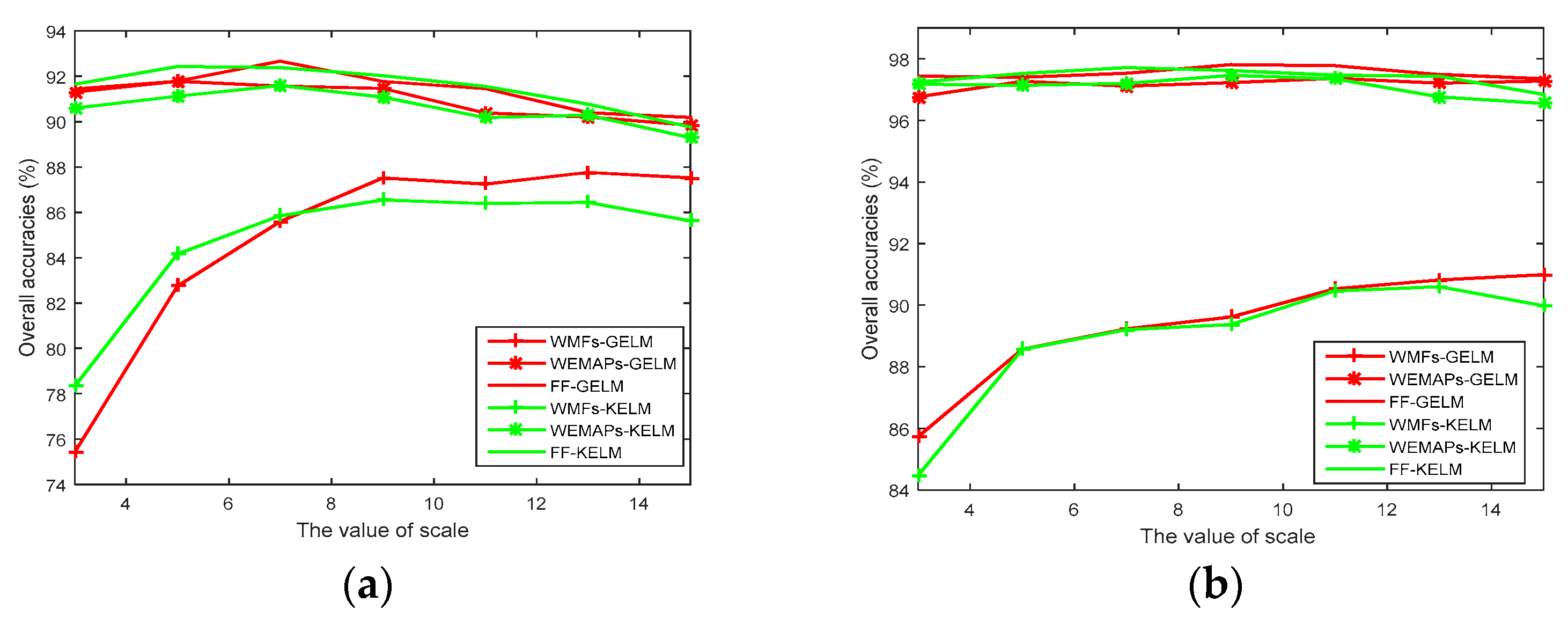
4.4. Investigation on the Effect of Scales

In this subsection, the impacts of the scales of the WMFs, proposed WEMAPs and FF on the GELM and KELM are investigated. Again, 15 training samples in each class are randomly selected for training and the remaining samples are used for testing. Figure 2 shows the classification results, where the following observations can be made: The proposed WEMAPs have better classification accuracies than WMFs and FF develop the classification accuracies of WEMAPs.

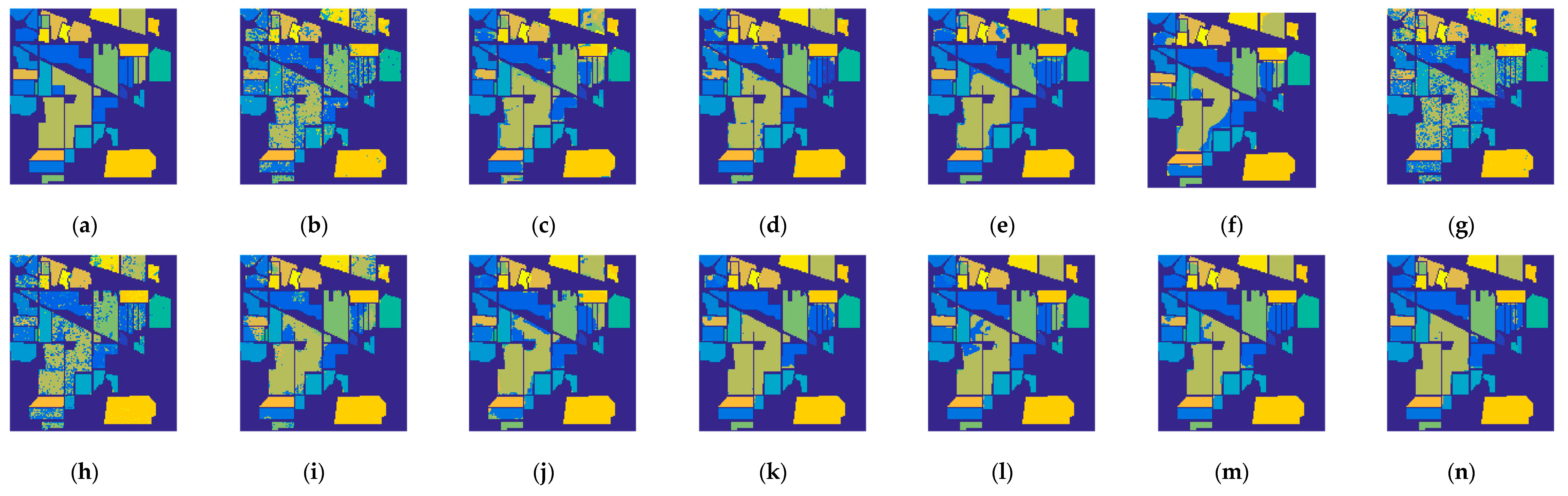
4.5. Classification Results and Comparisons on the Two Datasets

In this subsection, the performance of the proposed JDFFF is further evaluated by comparing with some well-known state-of-the-art approaches, where different numbers of samples are randomly chosen from each class for training, here Q = 5, 10, 15, 20, 25, 30. Note that the number of training samples in each class is capped to 50% if Q becomes more than half of the samples in that class. We also apply the proposed FF and JDFF to KSVM in order to show the good performance of proposed frameworks. For the JDFFF and FF, the scale is set to range from 3 to 9 and 3, respectively. For performance evaluation, four metrics are used including overall accuracies (OA), average accuracies (AA), kappa statistic (k) and standard deviation (S) [43].

Table 4. Classification accuracy (%) with different numbers of labeled samples for the Indian Pines dataset (the best result of each row is marked in bold).

Q	Index	KSVM	SVM-CKs	FF-KSVM	JDFFF-KSVM	SMLR-SPATV	GELM	KELM	GELM-CKs	KELM-CKs	FF-GELM	FF-KELM	JDFFF-GELM	JDFFF-KELM
5	OA	54.1 ± 4.1	59.18 ± 5.13	71.6 ± 2.9	74.5 ± 1.9	69.8 ± 5.7	50.8 ± 4.4	55.2 ± 3.8	62.3 ± 1.6	73.1 ± 2.8	80.3 ± 2.1	81.3 ± 2.1	82.3 ± 2.3	82.5 ± 2.7
	AA	66.1 ± 2.2	71.1 ± 2.8	80.9 ± 3.1	83.1 ± 1.4	80.8 ± 0.6	64.8 ± 3.5	68.3 ± 1.5	75.9 ± 1.6	83.1 ± 2.2	86.6 ± 1.8	87.4 ± 1.4	88.2 ± 1.3	88.3 ± 1.8
	k	48.8 ± 4.4	54.4 ± 5.5	68.2 ± 3.2	71.4 ± 2.1	66.3 ± 6.1	45.7 ± 0.2	50.3 ± 3.8	58.1 ± 1.8	69.8 ± 3.1	77.8 ± 2.4	78.9 ± 2.3	80.1 ± 2.6	80.3 ± 3.1
10	OA	64.3 ± 2.8	71.1 ± 4.1	79.3 ± 2.5	81.5 ± 2.8	77.8 ± 5.3	57.6 ± 2.9	63.3 ± 3.1	70.5 ± 1.7	80.9 ± 2.3	86.8 ± 1.9	88.2 ± 1.4	88.3 ± 2.1	88.8 ± 1.9
	AA	74.8 ± 2.1	81.5 ± 2.6	87.5 ± 0.9	89.4 ± 1.2	88.1 ± 1.9	70.8 ± 2.2	74.5 ± 2.2	82.8 ± 1.1	89.2 ± 1.5	92.1 ± 1.2	92.8 ± 0.9	93.1 ± 1.3	93.3 ± 1.1
	k	59.9 ± 3.1	67.7 ± 4.6	76.6 ± 2.8	79.2 ± 3.1	75.1 ± 5.7	52.6 ± 3.1	58.8 ± 3.2	67.1 ± 1.9	78.5 ± 2.5	85.1 ± 2.2	86.6 ± 1.6	86.7 ± 2.2	87.3 ± 2.1
15	OA	67.1 ± 2.4	78.7 ± 3.5	86.1 ± 1.9	86.9 ± 1.9	83.1 ± 2.4	61.1 ± 1.3	65.7 ± 3.3	77.7 ± 2.1	85.3 ± 2.1	91.8 ± 1.5	91.6 ± 2.2	92.5 ± 1.5	93.1 ± 1.1
	AA	77.6 ± 1.8	86.7 ± 1.9	91.5 ± 1.3	92.2 ± 1.2	91.6 ± 0.7	75.1 ± 0.9	77.9 ± 2.5	87.4 ± 0.8	92.1 ± 1.6	95.2 ± 0.9	95.1 ± 1.4	95.6 ± 0.8	96.1 ± 0.7
	k	63.2 ± 2.6	76.1 ± 3.9	84.3 ± 2.1	85.1 ± 2.1	81.1 ± 2.6	56.6 ± 1.3	61.7 ± 3.6	75.1 ± 2.2	83.4 ± 2.4	90.7 ± 1.7	90.5 ± 2.5	91.4 ± 1.7	92.1 ± 1.1
20	OA	71.1 ± 2.2	83.0 ± 2.4	88.1 ± 2.1	89.5 ± 1.2	85.9 ± 2.4	63.5 ± 1.4	70.8 ± 2.6	82.7 ± 1.7	89.6 ± 1.1	92.8 ± 1.2	93.5 ± 0.9	94.2 ± 0.9	94.1 ± 1.4
	AA	80.9 ± 1.3	89.6 ± 1.2	92.8 ± 1.2	93.8 ± 0.7	92.5 ± 1.0	77.2 ± 0.9	81.9 ± 1.0	91.1 ± 1.1	94.6 ± 0.7	95.7 ± 0.9	96.2 ± 0.6	96.6 ± 0.6	96.6 ± 0.9
	k	67.4 ± 2.5	80.8 ± 2.6	86.5 ± 2.2	88.1 ± 1.4	84.1 ± 2.6	59.3 ± 1.4	67.2 ± 2.8	80.5 ± 1.8	88.2 ± 1.1	91.8 ± 1.4	92.6 ± 1.1	93.4 ± 1.1	93.3 ± 1.6
25	OA	72.6 ± 1.8	85.5 ± 1.5	90.1 ± 1.1	90.5 ± 1.1	87.8 ± 2.1	66.5 ± 1.7	73.1 ± 2.3	85.9 ± 1.3	90.8 ± 1.1	93.1 ± 1.4	93.8 ± 1.1	93.8 ± 0.9	94.5 ± 1.1
	AA	82.5 ± 1.6	91.8 ± 1.1	94.1 ± 0.7	94.6 ± 0.8	93.8 ± 0.9	79.5 ± 0.8	83.8 ± 0.9	92.6 ± 0.9	95.5 ± 0.5	96.1 ± 1.1	96.5 ± 0.6	96.8 ± 0.6	97.1 ± 0.6
	k	69.1 ± 1.9	83.6 ± 1.7	88.7 ± 1.1	89.2 ± 1.2	86.2 ± 2.2	62.5 ± 1.7	69.7 ± 2.5	84.1 ± 1.5	89.6 ± 1.2	92.1 ± 1.6	92.9 ± 1.3	92.9 ± 1.1	93.8 ± 1.3
30	OA	74.4 ± 1.8	85.9 ± 1.8	90.6 ± 1.4	91.5 ± 1.1	89.1 ± 1.5	66.8 ± 0.6	74.3 ± 1.4	88.8 ± 1.6	91.9 ± 0.9	94.2 ± 1.1	94.9 ± 1.1	94.9 ± 1.1	95.1 ± 1.1
	AA	83.8 ± 1.2	92.1 ± 0.9	94.5 ± 0.6	95.2 ± 0.8	94.9 ± 5.6	79.7 ± 0.9	85.3 ± 1.1	94.3 ± 1.1	96.1 ± 0.7	96.8 ± 0.6	97.2 ± 0.5	97.3 ± 0.6	97.4 ± 0.6
	k	71.1 ± 1.9	84.1 ± 2.1	89.3 ± 1.6	90.3 ± 1.3	87.6 ± 1.6	63.1 ± 0.6	71.2 ± 1.5	87.3 ± 1.8	90.8 ± 1.1	93.4 ± 1.3	94.2 ± 1.1	94.2 ± 1.2	94.4 ± 1.3
	Time (s)	23.98	41.80	37.51	152.47	30.3	0.45	1.05	1.86	9.59	1.83	2.69	19.58	23.77

and

Table 5. Accuracy (%) with different numbers of labeled samples for the Pavia University dataset (the best result of each row is marked in bold).

Q	Index	KSVM	SVM-CKs	FF-KSVM	JDFFF-KSVM	SMLR-SPATV	GELM	KELM	GELM-CKs	KELM-CKs	FF-GELM	FF-KELM	JDFFF-GELM	JDFFF-KELM
5	OA	61.7 ± 10.7	63.3 ± 4.5	81.2 ± 2.6	84.76 ± 3.87	67.46 ± 6.94	60.9 ± 8.1	59.9 ± 6.7	63.2 ± 3.7	63.7 ± 8.1	88.8 ± 4.5	89.3 ± 5.4	91.61 ± 4.03	90.1 ± 3.1
	AA	73.1 ± 4.9	73.4 ± 3.3	86.4 ± 0.9	87.7 ± 2.1	76.1 ± 5.5	70.6 ± 4.6	71.9 ± 3.4	71.5 ± 2.2	72.5 ± 2.8	91.2 ± 2.2	91.5 ± 2.5	92.7 ± 1.8	91.9 ± 1.5
	k	53.1 ± 10.8	54.7 ± 4.7	76.1 ± 2.9	80.3 ± 4.6	59.3 ± 7.2	52.1 ± 8.3	51.1 ± 6.7	54.4 ± 3.5	55.2 ± 8.7	85.6 ± 5.5	86.27 ± 6.7	89.1 ± 5.1	87.2 ± 3.7
10	OA	71.2 ± 4.4	74.2 ± 6.7	87.7 ± 4.8	89.8 ± 4.2	77.4 ± 4.5	69.8 ± 4.3	67.6 ± 3.3	71.6 ± 3.5	75.7 ± 6.5	92.1 ± 3.3	92.00 ± 3.1	93.3 ± 3.7	93.7 ± 3.1
	AA	79.1 ± 1.9	79.9 ± 2.8	92.3 ± 2.4	93.5 ± 1.9	85.1 ± 2.4	77.9 ± 1.4	78.3 ± 1.9	77.2 ± 1.6	80.9 ± 3.2	95.4 ± 1.6	95.48 ± 1.9	95.9 ± 3.1	95.9 ± 3.1
	k	63.8 ± 4.8	67.3 ± 7.8	84.3 ± 5.9	86.9 ± 5.2	71.5 ± 4.8	62.2 ± 4.5	59.8 ± 3.5	63.9 ± 4.2	69.2 ± 7.9	89.7 ± 4.1	89.6 ± 3.8	91.3 ± 4.6	91.8 ± 3.7
15	OA	74.1 ± 6.4	85.7 ± 2.6	96.2 ± 1.1	97.1 ± 0.8	79.3 ± 3.1	74.7 ± 3.8	72.8 ± 4.3	76.1 ± 3.2	86.2 ± 3.4	97.4 ± 1.1	97.4 ± 0.8	97.9 ± 1.1	98.3 ± 0.9
	AA	81.1 ± 3.1	87.3 ± 1.3	96.7 ± 0.7	97.2 ± 0.6	86.1 ± 1.6	79.7 ± 1.2	81.2 ± 1.8	79.8 ± 1.8	87.2 ± 0.9	98.1 ± 0.8	97.9 ± 0.6	98.4 ± 0.5	98.5 ± 0.7
	k	67.2 ± 7.4	81.4 ± 3.3	95.1 ± 1.4	96.2 ± 1.2	73.8 ± 3.6	67.6 ± 4.2	65.7 ± 4.9	69.2 ± 3.7	82.1 ± 4.1	96.60 ± 1.5	96.6 ± 1.1	97.3 ± 1.4	97.7 ± 1.2
20	OA	75.9 ± 3.6	86.1 ± 2.9	96.1 ± 1.7	97.1 ± 2.1	85.3 ± 2.9	74.4 ± 3.1	75.3 ± 3.8	78.3 ± 1.1	86.1 ± 2.9	97.5 ± 1.6	97.5 ± 1.5	98.4 ± 1.5	98.3 ± 1.8
	AA	82.6 ± 1.1	88.2 ± 1.5	97.5 ± 0.5	97.9 ± 0.7	87.9 ± 2.6	80.4 ± 1.6	82.6 ± 1.6	82.4 ± 1.1	87.5 ± 2.1	98.3 ± 0.8	98.4 ± 0.5	98.9 ± 0.6	98.9 ± 0.6
	k	69.5 ± 4.1	81.9 ± 3.5	94.8 ± 2.2	96.2 ± 2.6	81.1 ± 3.6	67.6 ± 3.6	68.8 ± 4.3	72.1 ± 1.3	81.8 ± 3.7	96.7 ± 2.1	96.7 ± 2.1	97.9 ± 1.9	97.7 ± 2.3
25	OA	80.6 ± 2.3	87.2 ± 2.1	97.1 ± 1.0	98.1 ± 1.1	86.3 ± 5.3	77.3 ± 2.5	78.4 ± 3.2	79.5 ± 4.9	88.8 ± 1.8	98.6 ± 0.6	98.6 ± 0.7	99.2 ± 0.2	99.1 ± 0.4
	AA	85.5 ± 1.2	89.1 ± 1.3	97.9 ± 0.5	98.2 ± 0.8	90.2 ± 2.2	82.7 ± 1.4	84.9 ± 1.1	83.4 ± 1.6	89.9 ± 1.3	98.9 ± 0.4	99.1 ± 0.3	99.3 ± 0.2	99.3 ± 0.2
	k	75.1 ± 2.7	83.3 ± 2.6	96.2 ± 1.3	97.4 ± 1.4	82.5 ± 6.4	71.1 ± 2.8	72.6 ± 3.7	73.8 ± 5.7	85.3 ± 2.3	98.2 ± 0.8	98.1 ± 0.9	99.1 ± 0.3	98.9 ± 0.5
30	OA	81.8 ± 1.3	89.4 ± 1.8	97.7 ± 1.1	98.5 ± 0.6	90.1 ± 2.5	79.1 ± 1.7	80.9 ± 2.4	83.9 ± 1.9	90.9 ± 1.8	99.1 ± 0.5	98.7 ± 1.7	99.4 ± 0.3	99.3 ± 0.4
	AA	86.1 ± 0.8	90.6 ± 0.8	98.3 ± 0.6	98.6 ± 0.3	92.1 ± 1.9	83.6 ± 0.5	85.8 ± 0.8	85.6 ± 0.6	91.4 ± 1.2	99.3 ± 0.2	99.1 ± 0.8	99.4 ± 0.3	99.4 ± 0.1
	k	76.6 ± 1.5	86.1 ± 2.3	97.1 ± 1.3	98.1 ± 0.8	87.1 ± 3.1	73.1 ± 2.1	75.5 ± 2.9	79.1 ± 2.3	88.1 ± 2.4	98.8 ± 0.6	98.3 ± 2.2	99.2 ± 0.4	99.1 ± 0.5
	Time (s)	4.98	16.48	14.62	109.95	106.6	0.84	0.62	6.15	7.86	6.41	6.25	78.63	76.31

show the classification results for the Indian Pines dataset and the Pavia University dataset, respectively. Without loss of the generality, the average computational times of all the methods with 30 training samples are also listed in the tables for comparison. From these two tables, we can have the following observations:

(1) The proposed FF achieved better classification results compared with the CK and the MRF methods, which was further improved by the proposed JDFFF. Furthermore, we can also see that proposed FF-GELM and FF-KELM have produced better classification accuracies than FF-SVM. The same situations are happened to JDFFF methods, i.e., JDFFF-GELM, JDFFF-KELM and JDFFF-SVM.

(2) The proposed FF based on the ELM algorithms (the GELM and the KELM) have less computational times than other spectral spatial based SVM algorithms. This is because the proposed FF based on the ELM algorithms inherits the fast speed of the ELM. Additionally, the proposed JDFFF with the ELM algorithms (the GELM and the KELM) have the advantages of less computational time compared with other spectral spatial based SVM methods.

In addition, Figure 3 and Figure 4 show the results for the Indian Pines dataset and the Pavia University dataset with about 30 training samples per class.

5. Conclusions

In this paper, we propose a novel framework for HSI classification. First, an improved EMAPs, called the WEMAPs, is found to be able to better model the discriminant information and reduce the noise in the HSIs. Second, the features extracted by the WEMAPs and the WMFs are combined to obtain the better FF. Third, the proposed multiscale FF, namely the JDFFF, has further improved this HSI classification results. Finally, the GELM and KELM are applied to the proposed JDFFF for performing this HSI classification. Experimental results show a good performance of proposed framework.

In the future work, the dimension reduction [46] will be applied to further reduce the computational time of the proposed JDFFF. Additionally, the hyperspectral unmixing [47] will be explored to further improve the classification results.

References

1. Deng, C.; Liu, X. Active multi-kernel domain adaptation for hyperspectral image classification. Pattern Recognit. 2018, 77, 306–315. [Google Scholar] [CrossRef] [Green Version]
2. Torti, E.; Leon, R.; La, M. Parallel classification pipelines for skin cancer detection exploiting hyperspectral imaging on hybrid systems. Electronics 2020, 9, 1053. [Google Scholar] [CrossRef]
3. Zhou, Y.; Peng, J.; Chen, C.L.P. Dimension reduction using spatial and spectral regularized local discriminant embedding for hyperspectral image classification. IEEE Trans. Geosci. Remote Sens. 2015, 53, 1082–1095. [Google Scholar] [CrossRef]
4. Plaza, A.; Benediktsson, J.A.; Boardman, J.W. Recent advances in techniques for hyperspectral image processing. Remote Sens. Environ. 2019, 113, S110–S122. [Google Scholar] [CrossRef]
5. Hughes, G.F. On the mean accuracy of statistical pattern recognizers. IEEE Trans. Inform. Theory. 1968, 14, 55–63. [Google Scholar] [CrossRef] [Green Version]
6. Song, X.; Wu, L.; Hao, H. Hyperspectral image denoising based on spectral dictionary learning and sparse coding. Electronics 2019, 8, 86. [Google Scholar] [CrossRef] [Green Version]
7. Lin, L.; Chen, C.; Yang, J. Deep transfer HSI classification method based on information measure and optimal neighborhood noise reduction. Electronics 2019, 8, 1112. [Google Scholar] [CrossRef] [Green Version]
8. Kang, X.; Xiang, X.; Li, S.; Benediktsson, J.A. PCA-based edge-preserving features for hyperspectral image classification. IEEE Trans. Geosci. Remote Sens. 2017, 55, 7140–7151. [Google Scholar] [CrossRef]
9. Zabalza, J.; Ren, J.; Yang, M. Novel folded-PCA for improved feature extraction and data reduction with hyperspectral imaging and SAR in remote sensing. ISPRS J. Photogramm. Remote Sens. 2014, 93, 112–122. [Google Scholar] [CrossRef] [Green Version]
10. Mura, M.D.; Benediktsson, J.A.; Waske, B. Morphological attribute profiles for the analysis of very high resolution images. IEEE Trans. Geosci. Remote Sens. 2010, 48, 3747–3762. [Google Scholar] [CrossRef]
11. Mura, M.D.; Benediktsson, J.A.; Waske, B. Extended profiles with morphological attribute filters for the analysis of hyperspectral data. Int. J. Remote Sens. 2010, 31, 5975–5991. [Google Scholar] [CrossRef]
12. Jerome, H.F. Regularized discriminant analysis. J. Am. Stat. Assoc. 1989, 84, 165–175. [Google Scholar]
13. Kuo, B.C.; Landgrebe, D.A. Nonparametric weighted feature extraction for classification. IEEE Trans. Geosci. Remote Sens. 2004, 42, 1096–1105. [Google Scholar]
14. Zabalza, J.; Ren, J.; Zheng, J.; Zhao, H. Novel segmented stacked autoencoder for effective dimensionality reduction and feature extraction in hyperspectral imaging. Neurocomputing 2016, 185, 1–10. [Google Scholar] [CrossRef] [Green Version]
15. Yu, H.; Gao, L.; Li, J. Spectral-spatial hyperspectral image classification using subspace based support vector machines and adaptive markov random fields. Remote Sens. 2016, 8, 355. [Google Scholar] [CrossRef] [Green Version]
16. Samat, A.; Du, P.; Liu, S. Ensemble extreme learning machines for hyperspectral image classification. IEEE J. Sel. Top. Appl. Earth Obs. Remote Sens. 2014, 7, 1060–1069. [Google Scholar] [CrossRef]
17. Li, J.; Huang, X.; Gamba, P. Multiple feature learning for hyperspectral image classification. IEEE Trans. Geosci. Remote Sens. 2015, 53, 1592–1606. [Google Scholar] [CrossRef] [Green Version]
18. Cao, F.; Yang, Z.; Ren, J.; Ling, W.K. Extreme Sparse Multinomial Logistic Regression: A Fast and Robust Framework for Hyperspectral Image Classification. Remote Sens. 2017, 9, 1255. [Google Scholar] [CrossRef] [Green Version]
19. Torti, E.; Fontanella, A.; Plaza, A. Hyperspectral Image Classification Using Parallel Autoencoding Diabolo Networks on Multi-Core and Many-Core Architectures. Electronics 2018, 7, 411. [Google Scholar] [CrossRef] [Green Version]
20. Pesaresi, M.; Benediktsson, J.A. A new approach for the morphological segmentation of high-resolution satellite imagery. IEEE Trans. Geosci. Remote Sens. 2001, 39, 309–320. [Google Scholar] [CrossRef] [Green Version]
21. Benediktsson, J.A.; Palmason, J.A.; Sveinsson, J.R. Classification of hyperspectral data from urban areas based on extended morphological profiles. IEEE Trans. Geosci. Remote Sens. 2005, 43, 480–491. [Google Scholar] [CrossRef]
22. Xia, J.; Mura, M.D.; Chanussot, J. Random subspace ensembles for hyperspectral image classification with extended morphological attribute profiles. IEEE Trans. Geosci. Remote Sens. 2015, 53, 4768–4786. [Google Scholar] [CrossRef]
23. Mura, M.D.; Villa, A.; Benediktsson, J.A. Classification of hyperspectral images by using extended morphological attribute profiles and independent component analysis. IEEE Geosci. Remote Sens. Lett. 2011, 8, 542–546. [Google Scholar] [CrossRef] [Green Version]
24. Li, J.; Marpu, P.R.; Plaza, A. Generalized composite kernel framework for hyperspectral image classification. IEEE Trans. Geosci. Remote Sens. 2013, 51, 4816–4829. [Google Scholar] [CrossRef]
25. Li, W.; Prasad, S.; Fowler, J.E. Decision fusion in kernel-induced spaces for hyperspectral image classification. IEEE Trans. Geosci. Remote Sens. 2014, 52, 3399–3411. [Google Scholar] [CrossRef] [Green Version]
26. Li, W.; Chen, C.; Su, H. Local binary patterns and extreme learning machine for hyperspectral imagery classification. IEEE Trans. Geosci. Remote Sens. 2015, 53, 3681–3693. [Google Scholar] [CrossRef]
27. Prasad, S.; Bruce, L.M. Decision fusion with confidence-based weight assignment for hyperspectral target recognition. IEEE Trans. Geosci. Remote Sens. 2008, 46, 1448–1456. [Google Scholar] [CrossRef]
28. Lee, K.H. Combining Feature Fusion and Decision Fusion in Multimodal Biometric Authentication. J. Korea Inst. Inf Secur. Cryptol. 2010, 20, 133–138. [Google Scholar]
29. Sun, B.; Li, L.; Wu, X. Combining feature-level and decision-level fusion in a hierarchical classifier for emotion recognition in the wild. J. Multimodal User In. 2015, 10, 125–137. [Google Scholar] [CrossRef]
30. Liao, W.; Bellens, R.; Pizurica, A. Combining feature fusion and decision fusion for classification of hyperspectral and LiDAR data. In Proceedings of the 2014 IEEE Geoscience and Remote Sensing Symposium, Quebec City, QC, Canada, 13–18 July 2014; pp. 1241–1244. [Google Scholar]
31. Zhou, Y.; Peng, J.; Chen, C.L.P. Region-kernel-based support vector machines for hyperspectral image classification. IEEE Trans. Geosci. Remote Sens. 2015, 53, 4810–4824. [Google Scholar]
32. Soille, P. Morphological image analysis: Principles and applications. Sensor Rev. 1999, 28, 800–801. [Google Scholar]
33. Marpu, P.R.; Pedergnana, M.; Mura, M.D. Automatic generation of standard deviation attribute profiles for spectral–spatial classification of remote sensing data. IEEE Geosci. Remote Sens. Lett. 2013, 10, 293–297. [Google Scholar] [CrossRef]
34. Huang, G.B.; Zhu, Q.Y.; Siew, C.K. Extreme learning machine: Theory and applications. Neurocomputing 2006, 70, 489–501. [Google Scholar] [CrossRef]
35. Cao, F.; Yang, Z.; Ren, J.; Ling, W.K. Sparse Representation-Based Augmented Multinomial Logistic Extreme Learning Machine with Weighted Composite Features for Spectral-Spatial Classification of Hyperspectral Images. IEEE Trans. Geosci. Remote Sens. 2018, 56, 6263–6279. [Google Scholar] [CrossRef] [Green Version]
36. Huang, G.B.; Zhou, H.; Ding, X. Extreme learning machine for regression and multiclass classification. IEEE Trans. Syst. Man Cybern. B Cybern. 2012, 42, 513–529. [Google Scholar] [CrossRef] [Green Version]
37. Banerjee, K.S. Generalized Inverse of Matrices and its Applications; Wiley: Hoboken, HJ, USA, 1971. [Google Scholar]
38. Camps-Valls, G.; Gomez-Chova, L.; Muñoz-Marí, J. Composite kernels for hyperspectral image classification. IEEE Geosci. Remote Sens. Lett. 2006, 3, 93–97. [Google Scholar] [CrossRef]
39. Fletcher, R. Practical Methods of Optimization; Wiley: Hoboken, HJ, USA, 1980. [Google Scholar]
40. Huang, X.; Zhang, L. An SVM ensemble approach combining spectral, structural, and semantic features for the classification of high-resolution remotely sensed imagery. IEEE Trans. Geosci. Remote Sens. 2013, 51, 257–272. [Google Scholar] [CrossRef]
41. Ham, J.; Chen, Y.C.; Ghosh, J. Investigation of the random forest framework for classification of hyperspectral data. IEEE Geosci. Remote Sens. 2015, 43, 492–501. [Google Scholar] [CrossRef] [Green Version]
42. Bao, R.; Xia, J.; Du, P. Combining morphological attribute profiles via an ensemble method for hyperspectral image classification. IEEE Geosci. Remote Sens. Lett. 2016, 13, 359–363. [Google Scholar] [CrossRef]
43. Zhou, Y.; Peng, J.; Chen, C.L.P. Extreme learning machine with composite kernels for hyperspectral image classification. IEEE J. Sel. Topics Appl. Earth Observ. Remote Sens. 2015, 8, 2351–2360. [Google Scholar] [CrossRef]
44. Chang, C.C.; Lin, C.J. LIBSVM: A library for support vector machines. ACM 2011, 2, 1–39. [Google Scholar] [CrossRef]
45. Sun, L.; Wu, Z.; Liu, J. Supervised spectral–spatial hyperspectral image classification with weighted Markov random fields. IEEE Trans. Geosci. Remote Sens. 2015, 53, 1490–1503. [Google Scholar] [CrossRef]
46. Chen, W.; Yang, Z. Dimensionality Reduction Based on Determinantal Point Process and Singular Spectrum Analysis for Hyperspectral Images. IET Image Process. 2018, 13, 299–306. [Google Scholar] [CrossRef] [Green Version]
47. Li, J.; Bioucas-Dias, J.M.; Plaza, A. Robust collaborative nonnegative matrix factorization for hyperspectral unmixing. IEEE Trans. Geosci. Remote Sens. 2016, 54, 6076–6090. [Google Scholar] [CrossRef] [Green Version]
Figure 1. The flowchart of the proposed JDFFF framework for HSI classification.
Electronics 09 02137 g001
Figure 2. The impacts of the window scales of the WMFs, the proposed WEMAPs, the FF on the GELM and the KELM. (a) The classification results on Indian Pines dataset. (b) The classification results on the Pavia University dataset.
Electronics 09 02137 g002
Figure 3. Results for the Indian Pines dataset with about 30 training samples per class: (a) Ground truth. (b) KSVM (OA = 74.42). (c) SVM-CK (OA = 85.93). (d) FF-SVM (OA = 90.63). (e) JDFFF-SVM (OA = 91.54). (f) SMLR-SPATV (OA = 89.10). (g) GELM (OA = 66.85). (h) KELM (OA = 74.37). (i) GELM-CK (OA = 88.86). (j) KELM-CK (OA = 91.96). (k) GELM-FF (OA = 94.23). (l) KELM-FF (OA = 94.93). (m) GELM-JDFF (OA = 94.93). (n) KELM-JDFF (OA = 95.13).
Electronics 09 02137 g003
Figure 4. Results for the Pavia University dataset with about 30 training samples per class. (a) Ground truth. (b) KSVM (OA = 81.89). (c) SVM-CK (OA = 89.42). (d) FF-SVM (OA = 97.77). (e) JDFFF-SVM (OA = 98.50). (f) SMLR-SPATV (OA = 90.14). (g) GELM (OA = 79.16). (h) KELM (OA = 80.93). (i) GELM-CK (OA = 83.95). (j) KELM-CK (OA = 90.99). (k) GELM-FF (OA = 99.12). (l) KELM-FF (OA = 98.71). (m) GELM-JDFF (OA = 99.43). (n) KELM-JDFF (OA = 99.39).
Electronics 09 02137 g004