Some Algorithms for Computing Short-Length Linear Convolution

Abstract

In this article, we propose a set of efficient algorithmic solutions for computing short linear convolutions focused on hardware implementation in VLSI. We consider convolutions for sequences of length $N=$ 2, 3, 4, 5, 6, 7, and 8. Hardwired units that implement these algorithms can be used as building blocks when designing VLSI -based accelerators for more complex data processing systems. The proposed algorithms are focused on fully parallel hardware implementation, but compared to the naive approach to fully parallel hardware implementation, they require from 25% to about 60% less, depending on the length N and hardware multipliers. Since the multiplier takes up a much larger area on the chip than the adder and consumes more power, the proposed algorithms are resource-efficient and energy-efficient in terms of their hardware implementation.

1. Introduction

Discrete convolution is found in many applications in science and engineering. Above all, it plays a key role in modern digital signal and image processing. In digital signal processing, it is the basis of filtering, multiresolution decomposition, and optimization of the calculation of orthogonal transform [1,2,3,4,5,6,7,8,9,10]. In digital image processing, convolution is a basic operation of denoising, smoothing, edge detection, blurring, focusing, etc. [11,12,13]. There are two types of discrete convolutions: the cyclic convolution and the linear convolution. General principles for the synthesis of convolution algorithms were described in [1,2,3]. The main emphasis in these works was made primarily on the calculation of cyclic convolution, while in many digital signal and image processing applications, the calculation of linear convolutions is required.

In recent years, convolution has found unusually wide application in neural networks and deep learning. Among the various kinds of deep neural networks, convolutional neural networks (CNNs) are most widely used [14,15,16,17]. In CNNs, linear convolutions are the most computationally intensive operations, since in a typical implementation, their multiple computations occupy more than 90% of the CNN execution time [14]. Only one convolutional level in a typical CNN requires more than two thousand multiplications and additions. Usually, there are several such levels in the CNN. That is why developers of such type of networks seek and design efficient ways of implementing linear convolution using the smallest possible number of arithmetic operations.

To speed up linear convolution computation, various algorithmic methods have been proposed. The most common approach to effective calculating linear convolution is dipping it in the space of a double-size cyclic convolution with the subsequent application of a fast Fourier transform (FFT) algorithm [15,16,17]. The FFT-based linear convolution method is traditionally used for large length finite impulse response (FIR) filters; however, modern CNNs use predominantly small length FIR filters. In this situation, the most effective algorithms used in the computation of a small-length linear convolution are the Winograd-like minimal filtering algorithms [18,19,20], which are the most used currently. The algorithms compute linear convolution over small tiles with minimal complexity, which makes them more effective with small filters and small batch sizes; however, these algorithms do not calculate the whole convolution. They calculate only two inner products of neighboring vectors formed from the current data stream by a moving time window of length N; therefore, these algorithms do not compute the true linear convolution.

At the same time, there are a number of CNNs in which it is necessary to calculate full-size small-length linear convolutions. In addition, in many applications of digital signal processing, there is the problem of calculating a one-dimensional convolution using its conversion into a multidimensional convolution. The algorithm thus obtained has a modular structure, and each module calculates a short-length one-dimensional convolution [21].

The most popular sizes of sequences being convoluted are sequences of length 2, 3, 4, 5, 6, 7, and 8. However, in the papers known to the authors, there is no description of resource-efficient algorithms for calculation of linear convolutions for lengths greater than four [1,4,6,21,22]. In turn, the solutions given in the literature for N = 2, N = 3, and N = 4 do not give a complete imagination about the organization of the linear convolution calculation process, since their corresponding signal flow graphs are not presented anywhere. In this paper, we describe a complete set of solutions for linear convolution of small length N sequences from 2 to 8.

2. Preliminaries

Let $\left\{h_m\right\}$ and, $\left\{x_n\right\}$, $m=0,1,\dots ,M-1$, $n=0,1,\dots ,N-1$ be two finite sequences of length M and N, respectively. Their linear convolution is the sequence $\left\{y_1\right\}$, $i=0,1,\dots ,M+N-2$ defined by [1]:

$$y_i={\displaystyle \sum }_{n=0}^{N-1}{h}_{i-n}{x}_n,$$

(1)

where we take $h_{i-n}=0$, if $i-n<0$.

As a rule, the elements of one of the sequences to be convolved are constant numbers. For definiteness, we assume that it will be a sequence $\left\{h_m\right\}$.

Because sequences $\left\{x_n\right\}$ and $\left\{h_m\right\}$ are finite length, then their linear convolution (1) can also be implemented as matrix-vector multiplication:

$${\mathbf{Y}}_{(N+M-1)\times 1}={\mathbf{H}}_{(N+M-1)\times N}{\mathbf{X}}_{N\times 1}$$

(2)

where

$${\mathbf{H}}_{(N+M-1)\times N}=\left[\begin{array}{cccc}{h}_0& \hspace{1em}& & \\ h_1& h_0& \hspace{1em}& \\ ⋮& h_1& \ddots & \\ h_{M-1}& ⋮& \cdots & h_0\\ & h_{M-1}& \cdots & h_1\\ & \hspace{1em}& \ddots & ⋮\\ & \hspace{1em}& & h_{M-1}\end{array}\right],$$

(3)

$${\mathbf{X}}_{N\times 1}={[x_0,x_1,\dots x_{N-1}]}^{\mathrm{T}},$$

$${\mathbf{Y}}_{(N+M-1)\times 1}={[y_0,y_1,\dots ,y_{N+M-2}]}^{\mathrm{T}},$$

$${\mathbf{H}}_{M\times 1}={[h_0,h_1,\dots ,h_{M-1}]}^{\mathrm{T}}.$$

In the future, we assume that ${\mathbf{X}}_{N\times 1}$ is a vector of input data, ${\mathbf{Y}}_{(N+M-1)\times 1}$ is a vector of output data, and ${\mathbf{H}}_{M\times 1}$ is a vector containing constants.

Direct computation of (3) takes MN multiplications and (M − 1)(N − 1) addition. This means that the fully parallel hardware implementation of the linear convolution operation requires MN multipliers and N + M − 3 multi-input adders with a different number of inputs, which depends on the length of the sequences being convolved. Traditionally, the convolution for which M = N is assumed as a basic linear convolution operation. Resource-effective cyclic convolution algorithms for benchmark lengths (N = 2, 3,...,16) have long been published [1,2,3,4,5,6,7,8,9]. For linear convolution, optimized algorithms are described only for the cases N = 2, 3, 4 [4,6,21,22]. Below we show how to reduce the implementation complexity of some benchmark-lengths linear convolutions for the case of completely parallel hardware their implementation. For completeness, we also consider algorithms for the sequences of lengths M = N = 2, 3, and 4.

So, considering the above, the goal of this article is to develop and describe fully parallel resource-efficient algorithms for N = 2, 3, 4, 5, 6, 7, 8.

3. Algorithms for Short-Length Linear Convolution

The main idea of presented algorithm is to transform the linear convolution matrix into circular matrix and two Toeplitz matrices. Then we can rewrite (3) in following form:

$${\mathbf{Y}}_{(2N-1)\times 1}={\mathbf{H}}_{(2N-1)\times N}{\mathbf{X}}_{N\times 1}=\left[\left[\begin{array}{c}{\mathbf{H}}_{K\times N}\\ {\breve{\mathbf{H}}}_N\\ {\mathbf{H}}_{L\times N}\end{array}\right]-\left[\begin{array}{c}{\mathbf{0}}_{K\times N}\\ {\mathbf{H}}_{L\times N}\\ {\mathbf{0}}_{1\times N}\\ {\mathbf{H}}_{K\times N}\\ {\mathbf{0}}_{L\times N}\end{array}\right]\right]{\mathbf{X}}_{N\times 1}$$

(4)

where ${\mathbf{H}}_{K\times N}=\left[\begin{array}{cc}{\mathbf{T}}_K^{\left(l\right)}& {\mathbf{0}}_{K\times (N-K)}\end{array}\right]$ and ${\mathbf{H}}_{L\times N}=\left[\begin{array}{cc}{\mathbf{0}}_{L\times (N-L)}& {\mathbf{T}}_L^{\left(r\right)}\end{array}\right]$ are matrices that are horizontal concatenations of null matrices and left-triangular or right-triangular Toeplitz matrices, respectively:

$${\mathbf{T}}_{K\times N}^{\left(l\right)}=\left[\begin{array}{cccc}{h}_0& 0& \cdots & 0\\ h_1& h_0& \cdots & 0\\ ⋮& ⋮& \ddots & ⋮\\ h_{K-1}& h_{K-2}& \cdots & h_0\end{array}\right], {\mathbf{T}}_L^{\left(r\right)}=\left[\begin{array}{cccc}{h}_{N-1}& h_{N-2}& \cdots & h_{N-L-2}\\ 0& h_{N-1}& \cdots & h_{N-L-1}\\ ⋮& ⋮& \ddots & ⋮\\ 0& 0& \cdots & h_{N-1}\end{array}\right],$$

which gives

$${\mathbf{H}}_{K\times N}=\left[\begin{array}{cccccccc}{h}_0& 0& \cdots & 0& 0& 0& \cdots & 0\\ h_1& h_0& \cdots & 0& 0& 0& ⋮& 0\\ ⋮& ⋮& \ddots & ⋮& ⋮& ⋮& \ddots & ⋮\\ h_{K-1}& h_{K-2}& \cdots & h_0& 0& 0& \cdots & 0\end{array}\right],$$

$${\mathbf{H}}_{L\times N}=\left[\begin{array}{cc}\begin{array}{cccc}0& 0& \cdots & 0\\ 0& 0& \cdots & 0\\ ⋮& ⋮& \ddots & ⋮\\ 0& 0& \cdots & 0\end{array}& \begin{array}{cccc}{h}_{N-1}& h_{N-2}& \cdots & h_{N-L-2}\\ 0& h_{N-1}& \cdots & h_{N-L-1}\\ ⋮& ⋮& \ddots & ⋮\\ 0& 0& \cdots & h_{N-1}\end{array}\end{array}\right].$$

A circulant matrix ${\breve{\mathbf{H}}}_N$ is a matrix of cyclic convolution H_N with rows cyclically shifted by n positions down:

$${\breve{\mathbf{H}}}_N={\mathbf{I}}_N^{\left(\leftarrow n\right)}{\mathbf{H}}_N=\left[\begin{array}{cccc}{h}_K& h_{K-1}& \cdots & h_{K+1}\\ h_{K+1}& h_K& \cdots & h_{K+2}\\ ⋮& ⋮& \ddots & ⋮\\ h_{N-1}& h_{N-2}& \cdots & h_0\\ h_0& h_{N-1}& \cdots & h_1\\ ⋮& ⋮& \ddots & ⋮\\ h_{K-1}& h_{K-2}& \cdots & h_K\end{array}\right],$$

where ${\mathbf{I}}_N^{(\leftarrow n)}$- is permutation matrix obtained from the identity matrix by cyclic shift of its columns by n positions to the left and:

$${\mathbf{H}}_N=\left[\begin{array}{cccc}{h}_0& h_{N-1}& \cdots & h_1\\ h_1& h_0& \cdots & h_2\\ ⋮& ⋮& ⋮& ⋮\\ h_{N-1}& h_{N-2}& \cdots & h_0\end{array}\right].$$

The coefficients K and L are natural numbers arbitrary taken and fulfilling the dependence K + L = N − 1. These values are selected heuristically for each N separately.

The product ${\breve{\mathbf{H}}}_N{\mathbf{X}}_{N\times 1}$ is calculated using the well-known fast convolution algorithm. The products of ${\mathbf{H}}_{K\times N}{\mathbf{X}}_{N\times 1}$ and ${\mathbf{H}}_{L\times N}{\mathbf{X}}_{N\times 1}$ are also calculated using fast algorithms for matrix-vector multiplication with Toeplitz matrices. We use all of the above techniques to synthesize the final short-length linear convolution algorithms with reduced multiplicative complexity.

3.1. Algorithm for N = 2

Let ${\mathbf{X}}_{2\times 1}={[x_0,x_1]}^{\mathrm{T}}$ and ${\mathbf{H}}_{2\times 1}={[h_0,h_1]}^{\mathrm{T}}$ be 2-dimensional data vectors being convolved and ${\mathbf{Y}}_{3\times 1}={[y_0,y_1,y_2]}^{\mathrm{T}}$ be an input vector representing a linear convolution. The problem is to calculate the product

$${\mathbf{Y}}_{3\times 1}={\mathbf{H}}_{3\times 2}{\mathbf{X}}_{2\times 1},$$

(5)

where

$${\mathbf{H}}_{3\times 2}=\left[\begin{array}{cc}{h}_0& \\ h_1& h_0\\ & h_1\end{array}\right].$$

Direct computation of (5) takes four multiplications and one addition. It is easy to see that the matrix ${\mathbf{H}}_{3\times 2}$ possesses an uncommon structure. By the Toom–Cook algorithmic trick, the number of multiplications in the calculation of the 2-point linear convolution can be reduced [1,21].

With this in mind, the rationalized computational procedure for computing 2-point linear convolution has the following form:

$${\mathbf{Y}}_{3\times 1}={\mathbf{A}}_3^{\left(2\right)}{\mathbf{D}}_3{\mathbf{A}}_{3\times 2}^{\left(2\right)}{\mathbf{X}}_{2\times 1}$$

(6)

where

$${\mathbf{A}}_{3\times 2}^{\left(2\right)}=\left[\begin{array}{cc}1& \\ 1& -1\\ & 1\end{array}\right], {\mathbf{A}}_3^{\left(2\right)}=\left[\begin{array}{ccc}1& & \\ 1& -1& 1\\ & & 1\end{array}\right], {\mathbf{D}}_3=diag(h_0,h_0-h_1,h_1),$$

(7)

$$s_0^{\left(2\right)}=h_0, s_1^{\left(2\right)}=h_0-h_1, s_2^{\left(2\right)}=h_1.$$

(8)

Figure 1 shows a signal flow graph for the proposed algorithm, which also provides a simplified schematic view of a fully parallel processing unit for resource-effective implementing of 2-point linear convolution. In this paper, the all data flow graphs are oriented from left to right. Straight lines in the figures denote the data transfer (data path) operations. The circles in these figures show the operation of multiplication (multipliers in the case of hardware implementation) by a number inscribed inside a circle. Points where lines converge denote summation (adders in the case of hardware implementation) and dotted lines indicate the sign-change data paths (data paths with multiplication by −1). We use the usual lines without arrows on purpose, so as not to clutter the picture [23].

As it can be seen, the calculation of 2-point linear convolution requires only three multiplications and three additions. In terms of arithmetic units, a fully parallel hardware implementation of the processor unit for calculating a 2-point convolution will require three multipliers, one two-input adder, and one three-input adder. In terms of arithmetic units, a fully parallel hardware implementation of the processor unit for calculating a 2-point convolution will require three multipliers, one two-input adder, and one three-input adder instead of four multipliers and one two-input adder in the case of completely parallel implementation of (6). So, we exchanged one multiplier for one three-input adder.

3.2. Algorithm for N = 3

Let ${\mathbf{X}}_{3\times 1}={[x_0,x_1,x_2]}^{\mathrm{T}}$ and ${\mathbf{H}}_{3\times 1}={[h_0,h_1,h_2]}^{\mathrm{T}}$ be 3-dimensional data vectors being convolved and ${\mathbf{Y}}_{5\times 1}={[y_0,y_1,y_2,y_3,y_4]}^{\mathrm{T}}$ be an input vector represented linear convolution for N = 3. The problem is to calculate the product

$${\mathbf{Y}}_{5\times 1}={\mathbf{H}}_{5\times 3}{\mathbf{X}}_{3\times 1},$$

(9)

where

$${\mathbf{H}}_{5\times 3}=\left[\begin{array}{ccc}{h}_0& & \\ h_1& h_0& \\ h_2& h_1& h_0\\ & h_2& h_1\\ & & h_2\end{array}\right].$$

(10)

Direct computation of (9) takes nine multiplications and five addition. Because the matrix ${\mathbf{H}}_{5\times 3}$ also possesses uncommon structure, the number of multiplications in the calculation of the 3-point linear convolution can be reduced too [1,4,21].

An algorithm for computation 3-point linear convolution with reduced multiplicative complexity can be written with the help of following matrix-vector calculating procedure:

$${\mathbf{Y}}_{5\times 1}^{\left(3\right)}={\mathbf{A}}_{5\times 6}^{\left(3\right)}{\mathbf{D}}_6^{\left(3\right)}{\mathbf{A}}_{6\times 3}^{\left(3\right)}{\mathbf{X}}_{3\times 1},$$

(11)

where

$${\mathbf{A}}_{6\times 3}^{\left(3\right)}=\left[\begin{array}{ccc}1& & \\ & 1& \\ & & 1\\ 1& 1& \\ 1& & 1\\ & 1& 1\end{array}\right], {\mathbf{A}}_{5\times 6}^{\left(3\right)}=\left[\begin{array}{cccccc}1& & & & & \\ -1& -1& & 1& & \\ -1& 1& -1& & 1& \\ & -1& -1& & & 1\\ & & 1& & & \end{array}\right],$$

(12)

$${\mathbf{D}}_6^{\left(3\right)}=diag(h_0,h_1,h_2,h_0+h_1,h_0+h_2,h_1+h_2).$$

(13)

Figure 2 shows a signal flow graph of the proposed algorithm for the implementation of 3-point linear convolution. As it can be seen, the calculation of 3-point linear convolution requires only 6 multiplications and 10 additions. Thus, the proposed algorithm saves six multiplications at the cost of six extra additions compared to the ordinary matrix-vector multiplication method.

In terms of arithmetic units, a fully parallel hardware implementation of the processor unit for calculating a 3-point linear convolution (11) will require only six multipliers, four two-input adders, one three-input adder, and one four-input adder instead of 12 multipliers, 2 two-input adders, and 1 two-input adder in the case of fully parallel implementation of (9).

3.3. Algorithm for N = 4

Let ${\mathbf{X}}_{4\times 1}={[x_0,x_1,x_2,x_3]}^{\mathrm{T}}$ and ${\mathbf{H}}_{4\times 1}={[h_0,h_1,h_2,h_3]}^{\mathrm{T}}$ be 4-dimensional data vectors being convolved and ${\mathbf{Y}}_{7\times 1}={[y_0,y_1,y_2,y_3,y_4,y_5,y_6]}^{\mathrm{T}}$ be an input vector represented linear convolution for N = 4.

The problem is to calculate the product:

$${\mathbf{Y}}_{7\times 1}={\mathbf{H}}_{7\times 4}{\mathbf{X}}_{4\times 1},$$

(14)

where

$${\mathbf{H}}_{7\times 4}=\left[\begin{array}{cccc}{h}_0& & & \\ h_1& h_0& & \\ h_2& h_1& h_0& \\ h_3& h_2& h_1& h_0\\ & h_3& h_2& h_1\\ & & h_3& h_2\\ & & & h_3\end{array}\right].$$

Direct computation of (14) takes 16 multiplications and 9 addition. Due to the specific structure of matrix ${\mathbf{H}}_{7\times 4}$, the number of multiplication operations in the calculation of (14) can be significantly reduced.

An algorithm for computation 4-point linear convolution with reduced multiplicative complexity can be written using the following matrix-vector calculating procedure:

$${\mathbf{Y}}_{7\times 1}={\mathbf{A}}_{7\times 8}^{\left(4\right)}{\mathbf{A}}_{8\times 9}^{\left(4\right)}{\mathbf{D}}_9^{\left(4\right)}{\mathbf{A}}_{9\times 8}^{\left(4\right)}{\mathbf{A}}_{8\times 4}^{\left(4\right)}{\mathbf{X}}_{4\times 1},$$

(15)

where

$${\mathbf{A}}_{8\times 4}^{\left(4\right)}=\left[\begin{array}{cccc}1& & & \\ 1& & 1& \\ & 1& & 1\\ 1& & -1& \\ & 1& & -1\\ & & 1& \\ & & & 1\\ & & & 1\end{array}\right], {\mathbf{A}}_{9\times 8}^{\left(4\right)}=1\oplus {\mathbf{H}}_2\oplus \left[\begin{array}{cc}1& \\ & 1\\ 1& 1\end{array}\right]\oplus {\mathbf{I}}_3,$$

where ${\mathbf{I}}_N$ is anidentity $N\times N$ matrix, ${\mathbf{H}}_2$ is the $(2 \times 2)$ Hadamard matrix, and sign,”⊕” denotes direct sum of two matrices [23,24,25].

$${\mathbf{D}}_9^{\left(4\right)}=diag(s_0^{\left(4\right)}{s}_1^{\left(4\right)},\dots ,s_8^{\left(4\right)}),$$

$$s_0^{\left(4\right)}=h_0,s_1^{\left(4\right)}=(h_0+h_1+h_2+h_3)/4,s_2^{\left(4\right)}=(h_0-h_1+h_2-h_3)/4,$$

$$s_3^{\left(4\right)}=(h_0-h_1-h_2+h_3)/2,s_4^{\left(4\right)}=(h_0+h_1-h_2-h_3)/2,s_5^{\left(4\right)}=(h_0-h_2)/2,s_6^{\left(4\right)}=h_3,$$

$$s_7^{\left(4\right)}=h_2,s_8^{\left(4\right)}=h_3,$$

$${\mathbf{A}}_{8\times 9}^{\left(4\right)}=1\oplus {\mathbf{H}}_2\oplus \left[\begin{array}{ccc}& -1& 1\\ -1& & 1\end{array}\right]\oplus {\mathbf{I}}_3, {\mathbf{A}}_{7\times 8}^{\left(4\right)}=\left[\begin{array}{cccccccc}1& & & & & & & \\ & & 1& & 1& -1& -1& \\ & 1& & -1& & & & -1\\ & & 1& & -1& & & \\ -1& 1& & 1& & & & \\ & & & & & 1& 1& \\ & & & & & & & 1\end{array}\right].$$

Figure 3 shows a signal flow graph of the proposed algorithm for the implementation of 4-point linear convolution. So, the proposed algorithm saves 7 multiplications at the cost of 11 extra additions compared to the ordinary matrix-vector multiplication method.

In terms of arithmetic units, a fully parallel hardware implementation of the processor unit for calculating a 4-point linear convolution will require only 9 multipliers, 13 two-input adders, 2 three-input adders, and 1 four-input adder instead of 16 multipliers, 2 two-input adders, 2 three-input adders, and 1 four-input adder in the case of fully parallel implementation of (14).

3.4. Algorithm for N = 5

Let ${\mathbf{X}}_{5\times 1}={[x_0,x_1,x_2,x_3,x_4]}^{\mathrm{T}}$ and ${\mathbf{H}}_{5\times 1}={[h_0,h_1,h_2,h_3,h_4]}^{\mathrm{T}}$ be 5-dimensional data vectors being convolved and ${\mathbf{Y}}_{9\times 1}={[y_0,y_1,y_2,y_3,y_4,y_5,y_6,y_7,y_8]}^{\mathrm{T}}$ be an input vector representing a linear convolution for N = 5.

The problem is to calculate the product:

$${\mathbf{Y}}_{9\times 1}={\mathbf{H}}_{9\times 5}{\mathbf{X}}_{5\times 1},$$

(16)

where

$${\mathbf{H}}_{9\times 5}=\left[\begin{array}{cccc}{h}_0& & & \\ h_1& h_0& & \\ ⋮& h_1& \ddots & \\ h_4& ⋮& \ddots & h_0\\ & h_4& \ddots & h_1\\ & & \ddots & ⋮\\ & & & h_4\end{array}\right].$$

Direct computation of (16) takes 25 multiplications and 16 addition. Due to the specific structure of matrix ${\mathbf{H}}_{9\times 5}$, the number of multiplication operations in the calculation of (16) can be significantly reduced.

Thus, an algorithm for computation 5-point linear convolution with reduced multiplicative complexity can be written using the following matrix-vector calculating procedure:

$${\mathbf{Y}}_{9\times 1}={\mathbf{A}}_{9\times 11}^{\left(5\right)}{\mathbf{A}}_{11\times 13}^{\left(5\right)}{\mathbf{A}}_{13\times 16}^{\left(5\right)}{\mathbf{D}}_{16}^{\left(5\right)}{\mathbf{A}}_{16\times 15}^{\left(5\right)}{\mathbf{A}}_{15\times 11}^{\left(5\right)}{\mathbf{A}}_{11\times 5}^{\left(5\right)}{\mathbf{X}}_{5\times 1},$$

(17)

where

$${\mathbf{A}}_{11\times 5}^{\left(5\right)}=\left[\begin{array}{c}\begin{array}{ccccc}1& & & & \\ 1& & & {\mathbf{0}}_3& \\ & 1& & & \end{array}\\ \begin{array}{ccccc}1& & & & -1\\ & 1& & & -1\\ & & 1& & -1\\ & & & 1& -1\\ 1& 1& 1& 1& 1\end{array}\\ \begin{array}{ccccc}& & & 1& \\ & {\mathbf{0}}_3& & & 1\\ & & & & 1\end{array}\end{array}\right],{\mathbf{A}}_{15\times 11}^{\left(5\right)}=\left[\begin{array}{cc}\begin{array}{ccccccc}1& & & & & & \\ & 1& & & & & \\ & & 1& & & & \\ & & & 1& & & \\ & & & & 1& & \\ & & & 1& 1& & \\ & & & & & 1& \\ & & & & & & 1\\ & & & & & 1& 1\\ & & & 1& & -1& \\ & & & & 1& & -1\end{array}& {\mathbf{0}}_{11\times 4}\\ {\mathbf{0}}_{4\times 7}& {\mathbf{I}}_4\end{array}\right]$$

and ${\mathbf{0}}_{M\times N}$ is a null matrix of order $M\times N$ [23,24,25],

$${\mathbf{D}}_{16}^{\left(5\right)}=diag(s_0^{\left(5\right)}{s}_1^{\left(5\right)},\dots , s_{15}^{\left(5\right)}),$$

$$s_0^{\left(5\right)}=h_0,s_1^{\left(5\right)}=h_1,s_2^{\left(5\right)}=h_0,s_3^{\left(5\right)}=(h_0-h_2+h_3-h_4)/4,s_4^{\left(5\right)}=(h_1-h_2+h{}_3-h_4)/4,$$

$$s_5^{\left(5\right)}=(3h_2-2h_1+2h{}_0-2h_3+3h_4)/5,s_6^{\left(5\right)}=(-h_0+h_1-h{}_2+h_3),s_7^{\left(5\right)}=(-h_0+h_1-h{}_2+h_3),$$

$$s_8^{\left(5\right)}=(3h_0-2h_1+3h{}_2-2h_3-2h_4)/5,s_9^{\left(5\right)}=-h_2+h_3,s_{10}^{\left(5\right)}=h_1-h_2,$$

$$s_{11}^{\left(5\right)}=(-h_0-h_1+4h{}_2-h_3-h_4)/5,s_{12}^{\left(5\right)}=(h_0+h_1+h{}_2+h_3+h_4)/5,s_{13}^{\left(5\right)}=h_4,s_{14}^{\left(5\right)}=h_3,$$

$$s_{15}^{\left(5\right)}=h_4,$$

$${\mathbf{A}}_{16\times 15}^{\left(5\right)}=\left[\begin{array}{cc}\begin{array}{ccccccccccc}1& & & & & & & & & & \\ & 1& & & & & & & & & \\ & & 1& & & & & & & & \\ & & & 1& & & & & & & \\ & & & & 1& & & & & & \\ & & & & & 1& & & & & \\ & & & & & & 1& & & & \\ & & & & & & & 1& & & \\ & & & & & & & & 1& & \\ & & & & & & & & & 1& \\ & & & & & & & & & & 1\\ & & & & & 1& & & -1& & \end{array}& {\mathbf{0}}_{12\times 4}\\ {\mathbf{0}}_{4\times 11}& {\mathbf{I}}_4\end{array}\right],$$

$${\mathbf{A}}_{13\times 16}^{\left(5\right)}={\mathbf{I}}_3\oplus \left[\begin{array}{ccccccccc}1& & 1& & & & & & \\ & 1& 1& & & & & {\mathbf{0}}_3& \\ & & & 1& & 1& & & \\ & & & & 1& 1& & & \\ & {\mathbf{0}}_3& & & & & 1& & 1\\ & & & & & & & 1& 1\end{array}\right]\oplus {\mathbf{I}}_4,$$

$${\mathbf{A}}_{11\times 13}^{\left(5\right)}={\mathbf{I}}_3\oplus \left[\begin{array}{ccccccc}1& & & & -1& & 1\\ -1& -1& -1& -1& & & 1\\ & & & 1& & 1& 1\\ & & 1& & 1& & 1\\ & 1& & & & -1& 1\end{array}\right]\oplus {\mathbf{I}}_3,$$

$${\mathbf{A}}_{9\times 11}^{\left(5\right)}=\left[\begin{array}{ccccccccccc}1& & & & & & & & {\mathbf{0}}_{2\times 6}& & \\ & 1& 1& & & & & & & & \\ & & & & & 1& & & -1& -1& \\ & & {\mathbf{0}}_{3\times 5}& & & & 1& & & & -1\\ & & & & & & & 1& & & \\ -1& & & 1& & & & & \begin{array}{c}\hfill \\ {\mathbf{0}}_{2\times 6}\hfill \end{array}& & \\ & -1& -1& & 1& & & & & & \\ & & \begin{array}{c}\hfill \\ {\mathbf{0}}_{2\times 5}\hfill \end{array}& & & & & & 1& 1& \\ & & & & & & & & & & 1\end{array}\right].$$

Figure 4 shows a data flow diagram of the proposed algorithm for the implementation of 5-point linear convolution. The algorithm saves 9 multiplications at the cost of 22 extra additions compared to the ordinary matrix-vector multiplication method.

In terms of arithmetic units, a fully parallel hardware implementation of the processor unit for calculating a 5-point linear convolution will require 16 multipliers, 20 two-input adders, 2 three-input adders, 1 four-input adder, and 1 five-input adder instead of 25 multipliers, 2 two-input adders, 2 three-input adders, 2 four-input adders, and 1 five-input adder in the case of fully parallel implementation of expression (16).

3.5. Algorithm for N = 6

Let ${\mathbf{X}}_{6\times 1}={[x_0,x_1,x_2,x_3,x_4,x_5]}^{\mathrm{T}}$ and ${\mathbf{H}}_{6\times 1}={[h_0,h_1,h_2,h_3,h_4,h_5]}^{\mathrm{T}}$ be 6-dimensional data vectors being convolved and ${\mathbf{Y}}_{11\times 1}={[y_0,y_1,y_2,y_3,y_4,y_5,y_6,y_7,y_8,y_9,y_{10}]}^{\mathrm{T}}$ be an input vector representing a linear convolution for N = 6.

The problem is to calculate the product:

$${\mathbf{Y}}_{11\times 1}={\mathbf{H}}_{11\times 6}{\mathbf{X}}_{6\times 1},$$

(18)

where

$${\mathbf{H}}_{11\times 6}=\left[\begin{array}{cccc}{h}_0& & & \\ h_1& h_0& & \\ ⋮& h_1& \ddots & \\ h_5& ⋮& \ddots & h_0\\ & h_5& \ddots & h_1\\ & & \ddots & ⋮\\ & & & h_5\end{array}\right].$$

Direct computation of (18) takes 36 multiplications and 25 addition. We proposed an algorithm that takes only 16 multiplications and 44 additions. It saves 20 multiplications at the cost of 19 extra additions compared to the ordinary matrix-vector multiplication method.

Proposed algorithm for computation 6-point linear convolution can be written with the help of following matrix-vector calculating procedure:

$$Y{}_{11}^{\left(6\right)}={\mathbf{A}}_{11}^{\left(6\right)}{\breve{\mathbf{A}}}_{11}^{\left(6\right)}{\mathbf{A}}_{11\times 14}^{\left(6\right)}{\widehat{\mathbf{A}}}_{14}^{\left(6\right)}{\breve{\mathbf{A}}}_{14}^{\left(6\right)}{\mathbf{A}}_{14\times 16}^{\left(6\right)}{\mathbf{D}}_{16}^{\left(6\right)}{\mathbf{A}}_{16\times 14}^{\left(6\right)}{\breve{\mathbf{A}}}_{14}^{\left(6\right)}{\mathbf{A}}_{14}^{\left(6\right)}{\mathbf{A}}_{14\times 6}^{\left(6\right)}{\mathbf{X}}_{6\times 1},$$

(19)

where

$${\mathbf{A}}_{14\times 6}^{\left(6\right)}=\left[\begin{array}{cc}\begin{array}{ccc}1& & \\ 1& & \\ & 1& \\ 1& & \\ & & 1\end{array}& {\mathbf{0}}_{5\times 3}\\ {\mathbf{0}}_3& \begin{array}{ccc}& 1& \\ 1& & \\ & & 1\end{array}\\ \begin{array}{ccc}& 1& \end{array}& \begin{array}{ccc}& & \end{array}\\ {\mathbf{0}}_3& \begin{array}{ccc}1& & \\ & 1& \\ & & 1\end{array}\\ {\mathbf{0}}_{2\times 3}& \begin{array}{ccc}& 1& 1\\ & & 1\end{array}\end{array}\right],{\mathbf{A}}_{14}^{\left(6\right)}={\mathbf{I}}_3\oplus ({\mathbf{H}}_2\otimes {\mathbf{I}}_3)\oplus {\mathbf{I}}_5,$$

$${\breve{\mathbf{A}}}_{14}^{\left(6\right)}={\mathbf{I}}_3\oplus \left({\mathbf{I}}_2\otimes \left[\begin{array}{ccc}1& 1& 1\\ 1& -1& \\ 1& & -1\end{array}\right]\right)\oplus {\mathbf{I}}_5, {\mathbf{A}}_{16\times 14}^{\left(6\right)}={\mathbf{I}}_3\oplus \left({\mathbf{I}}_2\otimes \left[\begin{array}{ccc}1& & \\ & & 1\\ & 1& \\ & 1& 1\end{array}\right]\right)\oplus {\mathbf{I}}_5,$$

$${\mathbf{D}}_{16}=diag(s_0^{\left(6\right)},s_1^{\left(6\right)},\dots ,s_{15}^{\left(6\right)}),$$

$$\begin{array}{c}{s}_0^{\left(6\right)}=6h_0,s_1^{\left(6\right)}=6h_1,s_2^{\left(6\right)}=6h_0,s_3^{\left(6\right)}=h_0+h_3+h_4+h_1+h_2+h_5,\\ s_4^{\left(6\right)}=3(h_4+h_1-h_0-h_3),s_5^{\left(6\right)}=3(h_2+h_5-h_0-h_3),\\ s_6^{\left(6\right)}=3(h_0+h_3)-(h_0+h_3+h_4+h_1+h_2+h_5),s_7^{\left(6\right)}=h_0-h_3+h_4-h_1+h_2-h_5),\\ s_8^{\left(6\right)}=3(h_4-h_1-h_0+h_3),s_9^{\left(6\right)}=3(h_2-h_5-h_0+h_3),\\ s_{10}^{\left(6\right)}=3(h_0+h_3)-(h_0-h_3+h_4-h_1+h_2-h_5),s_{11}^{\left(6\right)}=6h_5,s_{12}^{\left(6\right)}=6(-h_4+h_5),\\ s_{13}^{\left(6\right)}=6(h_3-h_4),s_{14}^{\left(6\right)}=6h_4,s_{15}^{\left(6\right)}=6h_5,\end{array}$$

$${\mathbf{A}}_{14\times 16}^{\left(6\right)}={\mathbf{I}}_4\oplus \left[\begin{array}{ccc}\begin{array}{ccc}1& & 1\\ & 1& 1\end{array}& & {\mathbf{0}}_{2\times 4}\\ {\mathbf{0}}_{1\times 3}& 1& {\mathbf{0}}_{1\times 3}\\ {\mathbf{0}}_{2\times 4}& & \begin{array}{ccc}1& & 1\\ & 1& 1\end{array}\end{array}\right]\oplus {\mathbf{I}}_5,{\widehat{\mathbf{A}}}_{14}^{\left(6\right)}={\mathbf{I}}_4\oplus \left[\begin{array}{ccccc}& 1& & & \\ 1& & & & \\ & & 1& & \\ & & & & 1\\ & & & 1& \end{array}\right]\oplus {\mathbf{I}}_5,$$

$$\begin{array}{c}{\mathbf{A}}_{11\times 14}^{\left(6\right)}=\left[\begin{array}{ccc}1& & \\ & 1& 1\end{array}\right]\oplus ({\mathbf{H}}_2\otimes {\mathbf{I}}_3)\oplus \left[\begin{array}{ccccc}1& & 1& 1& \\ & 1& & 1& \\ & & & & 1\end{array}\right], {\breve{\mathbf{A}}}_{11}^{\left(6\right)}=\left[\begin{array}{ccc}{\mathbf{I}}_3& {\mathbf{0}}_{3\times 4}& {\mathbf{0}}_3\\ {\mathbf{0}}_{4\times 3}& \begin{array}{cccc}& & & 1\\ & 1& & \\ & & 1& \\ 1& & & \end{array}& {\mathbf{0}}_{4\times 3}\\ {\mathbf{0}}_{4\times 3}& {\mathbf{0}}_{4\times 3}& {\mathbf{I}}_4\end{array}\right],\end{array}$$

and sign “⊗” denotes tensor or Kronecker product of two matrices [23,24,25].

Figure 5 shows a data flow diagram of the proposed algorithm for the implementation of 6-point linear convolution.

In terms of arithmetic units, a fully parallel hardware implementation of the processor unit for calculating a 6-point linear convolution will require 16 multipliers, 32 two-input adders, and 5 three-input adders, instead of 36 multipliers, 2 two-input adders, 2 three-input adders, 2 four-input adders, 2 five-input adders, and 1 six-input adder in the case of completely parallel implementation of expression (18).

3.6. Algorithm for N = 7

Let ${\mathbf{X}}_{7\times 1}={[x_0,x_1,x_2,x_3,x_4.x_5,x_6]}^{\mathrm{T}}$ and ${\mathbf{H}}_{7\times 1}={[h_0,h_1,h_2,h_3,h_4,h_5,h_6]}^{\mathrm{T}}$ be 7-dimensional data vectors being convolved and ${\mathbf{Y}}_{13\times 1}={[y_0,y_1,y_2,y_3,y_4,y_5,y_6,y_7,y_8,y_9,y_{10},y_{11},y_{12}]}^{\mathrm{T}}$ be an input vector representing a linear convolution for N = 7.

The problem is to calculate the product:

$${\mathbf{Y}}_{13\times 1}={\mathbf{H}}_{13\times 7}{\mathbf{X}}_{7\times 1},$$

(20)

where

$${\mathbf{H}}_{13\times 7}=\left[\begin{array}{cccc}{h}_0& & & \\ h_1& h_0& & \\ ⋮& h_1& \ddots & \\ h_6& ⋮& \ddots & h_0\\ & h_6& \ddots & h_1\\ & & \ddots & ⋮\\ & & & h_6\end{array}\right].$$

Direct computation of (20) takes 49 multiplications and 36 addition. We developed an algorithm that contains only 26 multiplications and 79 additions. It saves 23 multiplications at the cost of 43 extra additions compared to the ordinary matrix-vector multiplication method.

The proposed algorithm for computation 7-point linear convolution with reduced multiplicative complexity can be written using the following matrix-vector calculating procedure:

$${\mathbf{Y}}_{13\times 1}^{\left(7\right)}={\mathbf{A}}_{13\times 26}^{\left(7\right)}{\mathbf{D}}_{26}^{\left(7\right)}{\mathbf{A}}_{26\times 7}^{\left(7\right)}{\mathbf{X}}_{7\times 1},$$

(21)

where

$${\mathbf{A}}_{13\times 26}^{\left(7\right)}={\mathbf{A}}_{13\times 15}^{\left(7\right)}{\mathbf{A}}_{15\times 20}^{\left(7\right)}{\mathbf{A}}_{20\times 21}^{\left(7\right)}{\mathbf{A}}_{21\times 22}^{\left(7\right)}{\mathbf{A}}_{22\times 25}^{\left(7\right)}{\mathbf{A}}_{25\times 21}^{\left(7\right)}{\mathbf{A}}_{21}^{\left(7\right)}{\mathbf{A}}_{21\times 26}^{\left(7\right)},$$

$${\mathbf{A}}_{26\times 7}^{\left(7\right)}={\mathbf{A}}_{26}^{\left(7\right)}{\mathbf{A}}_{26\times 28}^{\left(7\right)}{\mathbf{A}}_{28\times 21}^{\left(7\right)}{\mathbf{A}}_{21\times 18}^{\left(7\right)}{\mathbf{A}}_{18\times 7}^{\left(7\right)}$$

and

$$\begin{array}{c}{\mathbf{A}}_{18\times 7}^{\left(7\right)}=\left[\begin{array}{cc}\begin{array}{cccc}1& & & \\ 1& & & \\ & 1& & \\ 1& 1& & \\ & & 1& \\ 1& 1& 1& \end{array}& {\mathbf{0}}_{6\times 3}\\ {\mathbf{I}}_4& \begin{array}{cc}{\mathbf{0}}_{4\times 2}& -{\mathbf{1}}_{4\times 1}\end{array}\\ {\mathbf{0}}_{2\times 4}& \begin{array}{ccc}1& & -1\\ & 1& -1\end{array}\\ {\mathbf{0}}_{6\times 4}& \begin{array}{ccc}& & 1\\ & & 1\\ & & 1\\ & 1& \\ & 1& 1\\ 1& & \end{array}\end{array}\right],{\mathbf{A}}_{21\times 18}^{\left(7\right)}={\mathbf{I}}_5\oplus \left[\begin{array}{cccccccc}1& & & & & & & \\ 1& & & & & & & 1\\ & 1& & & & & & \\ & -1& & & 1& & & \\ & & & & 1& & & \\ & & 1& 1& & & & \\ & & -1& 1& & & & \\ & & & & & 1& 1& \\ & & & & & -1& 1& \\ & & & 1& & & & \\ & & & & & & 1& \end{array}\right]\oplus {\mathbf{I}}_5,\end{array}$$

$$-1_{4\times 1}={[-1,-1,-1,-1]}^{\mathrm{T}},$$

$${\mathbf{A}}_{28\times 21}^{\left(7\right)}={\mathbf{I}}_7\oplus \left[\begin{array}{cccccccccc}1& & & & & & & & & \\ & 1& & & & {\mathbf{0}}_{3\times 4}& & & {\mathbf{0}}_3& \\ & & 1& & & & & & & \\ 1& & & 1& & & & & & \\ 1& & & & 1& & & & {\mathbf{0}}_{4\times 3}& \\ & & 1& & & 1& & & & \\ & & 1& & & & 1& & & \\ & & & 1& & & & & & \\ & & & 1& & & & & & \\ & {\mathbf{0}}_{6\times 3}& & & 1& & & & {\mathbf{0}}_{6\times 3}& \\ & & & & & 1& & & & \\ & & & & & 1& & & & \\ & & & & & & 1& & & \\ & & & & & & & 1& & \\ & & & & & & & -1& 1& \\ & {\mathbf{0}}_{4\times 3}& & & & {\mathbf{0}}_4& & & 1& \\ & & & & & & & & & 1\end{array}\right]\oplus {\mathbf{I}}_4,$$

$${\mathbf{A}}_{26\times 28}^{\left(7\right)}={\mathbf{I}}_{10}\oplus \left[\begin{array}{cc}\begin{array}{cccc}1& & & \\ -1& & 1& \\ & 1& & \\ & & 1& \\ & -1& & 1\\ & & & 1\end{array}& {\mathbf{0}}_6\\ \begin{array}{cccc}1& \begin{array}{cc}& \end{array}& & \\ & & 1& \end{array}& \begin{array}{cccccc}1& 1& 1& & & \\ & & & 1& 1& 1\end{array}\end{array}\right]\oplus {\mathbf{I}}_8$$

$${\mathbf{A}}_{26}^{\left(7\right)}={\mathbf{I}}_5\oplus \left[\begin{array}{cc}\begin{array}{ccccccc}1& 1& & & & & 1\\ & & 1& & & & \\ & & & 1& & & \\ & & & & 1& & \\ & & & & & 1& \\ & & & & & & 1\end{array}& {\mathbf{0}}_6\\ {\mathbf{0}}_7& \begin{array}{cccccc}1& & & & & \\ & 1& & & & \\ & & 1& & & \\ & & & 1& & \\ & & & & 1& \\ & & & & -1& 1\\ & & & & & 1\end{array}\end{array}\right]\oplus {\mathbf{I}}_8,$$

$${\mathbf{D}}_{26}^{\left(7\right)}=diag(s_0^{\left(7\right)},s_1^{\left(7\right)},\dots ,s_{25}^{\left(7\right)}),$$

$$\begin{array}{c}{s}_0^{\left(7\right)}=h_0, s_1^{\left(7\right)}=h_2-h_1,s_2^{\left(7\right)}=h_0-h_1,s_3^{\left(7\right)}=h_1,s_4^{\left(7\right)}=h_0,\\ s_5^{\left(7\right)}=(h_6+h_5+h_4+h_3+2h_2+h_1+h_0)/7,s_6^{\left(7\right)}=(-h_6-2h_5+3h_4-h_3-2h_2+h_1+2h_0)/2,\\ s_7^{\left(7\right)}=(2h_4-h_3-2h_2+h_1)/2,s_8^{\left(7\right)}=(-h_6+h_5+2h_4-h_3-2h_2+3h_1-h_0)/2,\\ s_9^{\left(7\right)}=(10h_6+3h_5-11h_4+10h_3+3h_2-11h_1-4h_0)/14,\\ s_{10}^{\left(7\right)}=(-2h_6-2h_5-2h_4+12h_3+5h_2-9h_1-2h_0)/14,s_{11}^{\left(7\right)}=(2h_6+3h_5-h_4-2h_3+3h_2-h_1)/6,\\ s_{12}^{\left(7\right)}=(3h_6-11h_5-4h_4+10h_3+3h_2-11h_1+10h_0)/14,s_{13}^{\left(7\right)}=(-2h_3+3h_2-h_1)/6,\\ s_{14}^{\left(7\right)}=(3h_6-h_5-2h_3+3h_2-h_1-2h_0)/6,s_{15}^{\left(7\right)}=(-h_6+h_4-h_3+h_1)/6,s_{16}^{\left(7\right)}=(-h_3+h_1)/6,\\ s_{17}^{\left(7\right)}=(h_5-h_3+h_1-h_0)/6,s_{18}^{\left(7\right)}=2h_6-h_5-2h_4+3h_3-2h_2-2h_1+h_0,\\ s_{19}^{\left(7\right)}=2h_3-h_2-2h_1+h_0,s_{20}^{\left(7\right)}=-h_6-2h_5+h_4+2h_3-h_2-2h_1+3h_0,s_{21}^{\left(7\right)}=h_6,\\ s_{22}^{\left(7\right)}=h_4-h_5,s_{23}^{\left(7\right)}=h_6-h_5,s_{24}^{\left(7\right)}=h_5,s_{25}^{\left(7\right)}=h_6,\end{array}$$

$${\mathbf{A}}_{21\times 26}^{\left(7\right)}={\mathbf{I}}_6\oplus \left[\begin{array}{cc}\begin{array}{ccccccccc}1& 1& & & & & & & \\ & & & 1& 1& & & & \\ & & & & & 1& & 1& \end{array}& {\mathbf{0}}_{3\times 6}\\ {\mathbf{0}}_{2\times 9}& \begin{array}{cccccc}1& 1& & & & \\ & & & 1& 1& \end{array}\\ \begin{array}{ccccccccc}& -1& 1& & & & & & \\ & & & & -1& & 1& & \\ & & & & & & & -1& 1\end{array}& {\mathbf{0}}_{3\times 6}\\ {\mathbf{0}}_{2\times 9}& \begin{array}{cccccc}& -1& 1& & & \\ & & & & -1& 1\end{array}\end{array}\right]\oplus {\mathbf{I}}_5,$$

$$\begin{array}{c}{\mathbf{A}}_{21}^{\left(7\right)}={\mathbf{I}}_7\oplus \left[\begin{array}{cc}\begin{array}{cccc}1& & 1& \\ & 1& & \\ & & 1& \\ & & & 1\end{array}& {\mathbf{0}}_4\\ {\mathbf{0}}_4& \begin{array}{cccc}1& & & \\ & 1& & 1\\ & & 1& \\ & & & 1\end{array}\end{array}\right]\oplus {\mathbf{I}}_6, {\mathbf{A}}_{25\times 21}^{\left(7\right)}={\mathbf{I}}_7\oplus \left[\begin{array}{cc}\begin{array}{cccc}1& 1& & \\ 1& & 1& \\ & 1& & \\ & & 1& \\ & & 1& \\ & & & 1\end{array}& {\mathbf{0}}_{6\times 4}\\ {\mathbf{0}}_{6\times 4}& \begin{array}{cccc}1& & & \\ & 1& & \\ & 1& & 1\\ & & 1& \\ & & & 1\\ & & & 1\end{array}\end{array}\right]\oplus {\mathbf{I}}_6,\end{array}$$

$${\mathbf{A}}_{22\times 25}^{\left(7\right)}={\mathbf{I}}_6\oplus \left[\begin{array}{cc}\begin{array}{ccccccc}1& 1& & & & & \\ & & 1& & & {\mathbf{0}}_3& \\ & & 1& -1& & & \\ & & 1& & 1& 1& 1\\ & & & 1& & & \end{array}& {\mathbf{0}}_{5\times 7}\\ {\mathbf{0}}_{6\times 7}& \begin{array}{ccccccc}1& & & & & & \\ & 1& & & & {\mathbf{0}}_3& \\ & & 1& & & & \\ & & 1& -1& & & \\ & & 1& & 1& 1& 1\\ & & & 1& & & \end{array}\end{array}\right]\oplus {\mathbf{I}}_5,$$

$$\begin{array}{c}{\mathbf{A}}_{21\times 22}^{\left(7\right)}={\mathbf{I}}_6\oplus \left[\begin{array}{cc}\begin{array}{cccccc}1& & & & & \\ -1& -1& & -1& & \\ & & 1& & & \\ & & & 1& 1& \\ & & & & & 1\end{array}& {\mathbf{0}}_5\\ {\mathbf{0}}_{5\times 6}& \begin{array}{ccccc}& 1& & & \\ & & 1& & \\ & & & 1& 1\\ & & & & 1\\ & & & 1& \end{array}\end{array}\right]\oplus {\mathbf{I}}_5, {\mathbf{A}}_{20\times 21}^{\left(7\right)}={\mathbf{I}}_{10}\oplus \left[\begin{array}{ccccc}1& & & & 1\\ & 1& & & \\ & & 1& & \\ & & & 1& \end{array}\right]\oplus {\mathbf{I}}_6,\end{array}$$

$${\mathbf{A}}_{15\times 20}^{\left(7\right)}=\left[\begin{array}{ccccc}1& & & & \\ & & 1& 1& \\ & 1& & 1& 1\end{array}\right]\oplus {\mathbf{I}}_5\oplus \left[\begin{array}{cc}\begin{array}{ccccc}1& & & & \\ -1& -1& & & -1\\ & & 1& & \\ & & & 1& \end{array}& {\mathbf{0}}_{4\times 5}\\ {\mathbf{0}}_{3\times 5}& \begin{array}{ccccc}1& & & 1& 1\\ & & 1& 1& \\ 1& & & & \end{array}\end{array}\right],$$

$${\mathbf{A}}_{13\times 15}^{\left(7\right)}=\left[\begin{array}{cccc}{\mathbf{I}}_3& {\mathbf{0}}_{3\times 4}& {\mathbf{0}}_{3\times 5}& {\mathbf{0}}_3\\ {\mathbf{0}}_{4\times 3}& \begin{array}{cccc}1& & & \\ 1& & & \\ 1& & & \\ 1& & & 1\end{array}& \begin{array}{cccc}& & & 1\\ & 1& & \\ 1& & & \\ & & & \end{array}& \begin{array}{ccc}-1& & \\ & -1& \\ & & -1\\ & & \end{array}\\ \begin{array}{cccc}-1& & & 1\\ & -1& & 1\\ & & -1& 1\end{array}& \begin{array}{ccc}1& & \\ & 1& \begin{array}{cc}& \end{array}\\ & & \end{array}& \begin{array}{ccccc}& & & & \\ & & 1& & \\ & & & & 1\end{array}& {\mathbf{0}}_3\\ {\mathbf{0}}_{3\times 4}& {\mathbf{0}}_3& {\mathbf{0}}_{3\times 5}& {\mathbf{I}}_3\end{array}\right],$$

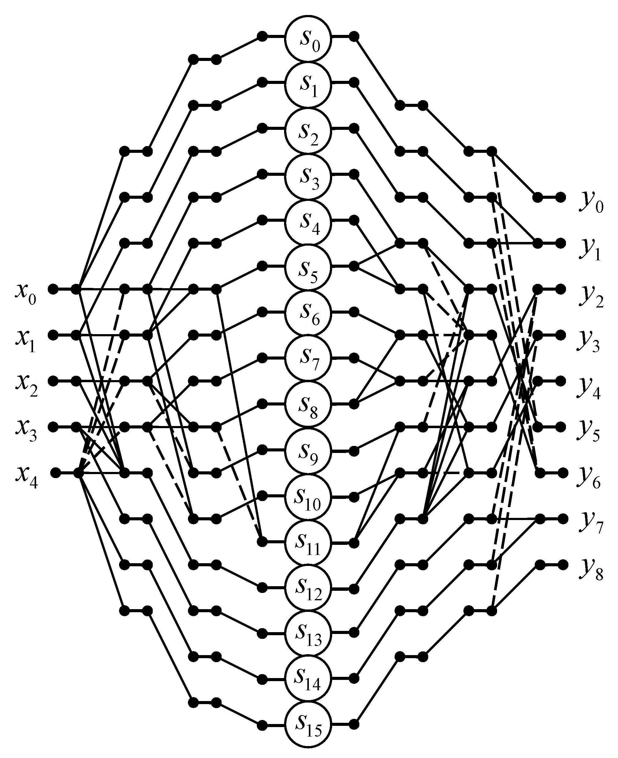
Figure 6 shows a data flow diagram of the proposed algorithm for the implementation of 7-point linear convolution.

In terms of arithmetic units, a fully parallel hardware implementation of the processor unit for calculating a 7-point linear convolution will require 27 multipliers, 49 two-input adders, 7 three-input adders, and 5 four-input adders, instead of 49 multipliers, 2 two-input adders, 2 three-input adders, 2 four-input adders, 2 five-input adders, 2 six-input adders, and 1 seven-input adder in the case of completely parallel implementation of expression (20).

3.7. Algorithm for N = 8

Let ${\mathbf{X}}_{8\times 1}={[x_0,x_1,x_2,x_3,x_4.x_5,x_6,x_7]}^{\mathrm{T}}$ and ${\mathbf{H}}_{8\times 1}={[h_0,h_1,h_2,h_3,h_4,h_5,h_6,h_7]}^T$ be 8-dimensional data vectors being convolved and ${\mathbf{Y}}_{15\times 1}={[y_0,y_1,y_2,y_3,y_4,y_5,y_6,y_7,y_8,y_9,y_{10},y_{11},y_{12},y_{13},y_{14}]}^T$ be an input vector representing a linear convolution for N = 8.

The problem is to calculate the product:

$${\mathbf{Y}}_{15\times 1}={\mathbf{H}}_{15\times 8}{\mathbf{X}}_{8\times 1},$$

(22)

where

$${\mathbf{H}}_{15\times 8}=\left[\begin{array}{cccc}{h}_0& & & \\ h_1& h_0& & \\ ⋮& h_1& \ddots & \\ h_7& ⋮& \ddots & h_0\\ & h_7& \ddots & h_1\\ & & \ddots & ⋮\\ & & & h_7\end{array}\right].$$

Direct computation of (22) takes 64 multiplications and 49 addition. We developed an algorithm that contains only 27 multiplications and 67 additions. Thus, the proposed algorithm saves 22 multiplications at the cost of 18 extra additions compared to the ordinary matrix-vector multiplication method.

Proposed algorithm for computation 8-point linear convolution with reduced multiplicative complexity can be written using the following matrix-vector calculating procedure:

$${\mathbf{Y}}_{15\times 1}={\mathbf{A}}_{15}^{\left(8\right)}{\widehat{\mathbf{A}}}_{15}^{\left(8\right)}{\breve{\mathbf{A}}}_{15}^{\left(8\right)}{\mathbf{A}}_{15\times 17}^{\left(8\right)}{\mathbf{A}}_{17\times 27}^{\left(8\right)}{\mathbf{D}}_{27}^{\left(8\right)}{\mathbf{A}}_{27\times 17}^{\left(8\right)}{\mathbf{A}}_{17\times 15}^{\left(8\right)}{\mathbf{A}}_{15\times 8}^{\left(8\right)}{\mathbf{X}}_{8\times 1}$$

(23)

where

$${\mathbf{A}}_{15\times 8}^{\left(8\right)}=\left[\begin{array}{cc}{\mathbf{I}}_3& {\mathbf{0}}_{3\times 5}\\ {\mathbf{I}}_4& {\mathbf{I}}_4\\ {\mathbf{I}}_4& -{\mathbf{I}}_4\\ {\mathbf{0}}_4& {\mathbf{I}}_4\end{array}\right], {\mathbf{A}}_{17\times 15}^{\left(8\right)}={\mathbf{I}}_3\oplus ({\mathbf{H}}_2\otimes {\mathbf{I}}_2)\oplus \left[\begin{array}{cc}{\mathbf{I}}_2& {\mathbf{0}}_2\\ {\mathbf{0}}_2& {\mathbf{I}}_2\\ {\mathbf{I}}_2& {\mathbf{I}}_2\end{array}\right]\oplus {\mathbf{I}}_4,$$

$${\mathbf{A}}_{27\times 17}^{\left(8\right)}=\left[\begin{array}{ccc}1& & \\ 1& & \\ & 1& \\ 1& 1& \\ & & 1\end{array}\right]\oplus {\mathbf{H}}_2\oplus \left({\mathbf{I}}_4\otimes \left[\begin{array}{cc}1& \\ & 1\\ 1& 1\end{array}\right]\right)\oplus \left[\begin{array}{cccc}& & & 1\\ & 1& 1& 1\\ & 1& -1& 1\\ & 1& & \\ 1& & & \\ & & & 1\\ & & & 1\\ & & 1& \end{array}\right],$$

$${\mathbf{D}}_{27}^{\left(8\right)}=diag(s_0^{\left(8\right)},s_1^{\left(8\right)},...,s_{27}^{\left(8\right)}),$$

$$\begin{array}{c}{s}_0^{\left(8\right)}=h_0,s_1^{\left(8\right)}=h_2-h_1,s_2^{\left(8\right)}=h_0-h_1,s_3^{\left(8\right)}=h_1,s_4^{\left(8\right)}=h_0,\\ s_5^{\left(8\right)}=\frac{1}{8}(h_0+h_1+h_2+h_3+h_4+h_5+h_6+h_7),s_6^{\left(8\right)}=\frac{1}{8}(h_0-h_1+h_2-h_3+h_4-h_5+h_6-h_7),\\ s_7^{\left(8\right)}=\frac{1}{4}(-h_0+h_1+h_2-h_3-h_4+h_5+h_6-h_7),s_8^{\left(8\right)}=\frac{1}{4}(-h_0-h_1+h_2+h_3-h_4-h_5+h_6+h_7),\\ s_9^{\left(8\right)}=\frac{1}{4}(h_0-h_2+h_4-h_6),s_{10}^{\left(8\right)}=\frac{1}{2}(h_0-h_1-h_2+h_3-h_4+h_5+h_6-h_7),\\ s_{11}^{\left(8\right)}=\frac{1}{2}(h_0+h_1-h_2+h_3-h_4-h_5+h_6-h_7),s_{12}^{\left(8\right)}=\frac{1}{2}(-h_0+h_2+h_4-h_6),\\ s_{13}^{\left(8\right)}=\frac{1}{2}(h_0-h_1+h_2-h_3-h_4+h_5-h_6+h_7),s_{14}^{\left(8\right)}=\frac{1}{2}(h_0-h_1+h_2+h_3-h_4+h_5-h_6-h_7),\\ s_{15}^{\left(8\right)}=\frac{1}{2}(-h_0-h_2+h_4+h_6),s_{16}^{\left(8\right)}=\frac{1}{2}(-h_0+h_1+h_4-h_5),s_{17}^{\left(8\right)}=\frac{1}{2}(-h_0-h_3+h_4+h_7),\\ s_{18}^{\left(8\right)}=\frac{1}{2}(h_0-h_4),s_{19}^{\left(8\right)}=h_4-h_6,s_{20}^{\left(8\right)}=\frac{1}{2}(h_5+h_6),s_{21}^{\left(8\right)}=\frac{1}{2}(h_6-h_5),s_{22}^{\left(8\right)}=h_5-h_7,\\ s_{23}^{\left(8\right)}=h_7,s_{24}^{\left(8\right)}=h_6,s_{25}^{\left(8\right)}=h_7,s_{26}^{\left(8\right)}=h_7,\end{array}$$

$$\begin{array}{c}{\mathbf{A}}_{17\times 27}^{\left(8\right)}=\left[\begin{array}{ccccc}1& & & & \\ & & 1& 1& \\ & 1& & 1& 1\end{array}\right]\oplus {\mathbf{H}}_2\oplus \left({\mathbf{I}}_4\otimes \left[\begin{array}{ccc}& 1& 1\\ 1& & 1\end{array}\right]\right)\oplus \left[\begin{array}{ccccc}1& 1& 1& & 1\\ & 1& -1& -1& \end{array}\right]\oplus \left[\begin{array}{ccc}1& & 1\\ & 1& \end{array}\right],\end{array}$$

$${\mathbf{A}}_{15\times 17}^{\left(8\right)}={\mathbf{I}}_3\oplus ({\mathbf{H}}_2\otimes {\mathbf{I}}_2)\oplus \left[\begin{array}{ccc}{\mathbf{0}}_2& {\mathbf{I}}_2& {\mathbf{I}}_2\\ {\mathbf{I}}_2& {\mathbf{0}}_2& {\mathbf{I}}_2\end{array}\right]\oplus {\mathbf{I}}_4, {\breve{\mathbf{A}}}_{15}^{\left(8\right)}={\mathbf{I}}_3\oplus ({\mathbf{H}}_2\otimes {\mathbf{I}}_4)\oplus {\mathbf{I}}_4,$$

$${\widehat{\mathbf{A}}}_{15}^{\left(8\right)}={\mathbf{I}}_3\oplus \left[\begin{array}{cc}{\mathbf{0}}_{5\times 3}& {\mathbf{I}}_5\\ {\mathbf{I}}_3& {\mathbf{0}}_{3\times 5}\end{array}\right]\oplus {\mathbf{I}}_4, {\mathbf{A}}_{15}^{\left(8\right)}=\left[\begin{array}{cc}{\mathbf{I}}_7& {\mathbf{0}}_{3\times 4}\oplus (-{\mathbf{I}}_4)\\ \left[\begin{array}{ccc}& & \\ -1& & \\ & -1& \\ & & -1\end{array}\right]\oplus {\mathbf{I}}_4& {\mathbf{I}}_8\end{array}\right].$$

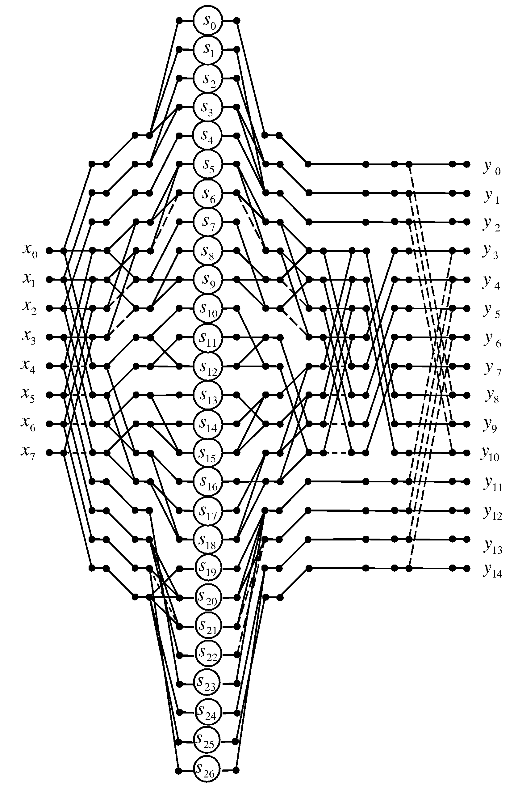
Figure 7 shows a data flow diagram of the proposed algorithm for the implementation of 8-point linear convolution.

In terms of arithmetic units, a fully parallel hardware implementation of the processor unit for calculating a 8-point linear convolution will require 27 multipliers, 57 two-input adders, 4 three-input adders and 1 four-input adder, instead of 64 multipliers, 2 two-input adders, 2 three-input adders, 2 four-input adders, 2 five-input adders, 2 six-input adders, 2 seven-point adders and 1 eight-input adder in the case of completely parallel implementation of expression (22).

4. Implementation Complexity

Since the lengths of the input sequences are relatively small, and the data flow graphs representing the organization of the computation process are fairly simple, it is easy to estimate the implementation complexity of the proposed solutions.

Table 1. Implementation complexities of naïve method and proposed solutions.

Length N	Number of Arithmetical Units (Multipliers — “×” and Adders — “+”)
	Naïve Method		Proposed Solutions		Percentage Stimate
	“×”	“+”	“×”	“+”	“×"	“+”
2	4	1	3	3	25%	66.7%
3	9	4	6	10	33.3%	60%
4	16	9	9	20	43.8%	55%
5	25	16	16	38	57.9%	66%
6	36	25	16	44	55.6%	43.2%
7	49	36	26	79	47%	54.4%
8	64	49	27	67	58%	26.9%

shows estimates of the number of arithmetic blocks for the fully parallel implementation of the short lengths linear convolution algorithms. Since a parallel N-input adder consists of N-1 two-input adders, we give integrated estimates of the implementing costs of the sets of adders for each proposed solution expressed as the sums of two-input adders. The penultimate column of the Table 1 shows the percentage reduction in the number of multipliers, while the last column shows the percentage increase in the number of adders. As you can see, the implementation of the proposed algorithms requires fewer multipliers than the implementation based on naive methods of performing the linear convolution operations.

It should be noted that our solutions are primarily focused on efficient implementation in application specific integrated circuits (ASICs). In low-power designing low-power digital circuits, optimization must be performed both at the algorithmic level and at the logic level. From the point of view of designing an ASIC-chip that implements fast linear convolution, you should pay attention to the fact that the hardwired multiplier is a very resource-intensive arithmetic unit. The multiplier is also the most energy-intensive arithmetic unit, occupying a large crystal area [26] and dissipating a lot of energy [27]. Reducing the number of multipliers is especially important in the design of specialized fully parallel ASIC-based processors because minimizing the number of necessary multipliers reduces power dissipation and lowers the cost implementation of the entire system being implemented. It is proved that the implementation complexity of a hardwired multiplier grows quadratically with operand size, while the hardware complexity of a binary adder increases linearly with operand size [28]. Therefore, a reduction in the number of multipliers, even at the cost of a small increase in the number of adders, has a significant role in the ASIC-based implementation of the algorithm. Thus, it can be argued categorically that algorithmic solutions that require fewer hardware multipliers in an ASIC-based implementation are better than those that require more embedded multipliers.

This statement is also true for field-programmable gate array (FPGA)-based implementations. Most modern high-performance FPGAs contain a number of built-in multipliers. This means that instead of implementing the multipliers with a help of a set of conventional logic gates, you can use the hardwired multipliers embedded in the FPGA. Thus, all multiplications contained in a fully parallel algorithm can be efficiently implemented using these embedded multipliers; however, their number may not be enough to meet the requirements of a fully parallel implementation of the algorithm. So, the developer uses the embedded multipliers to implement the multiplication operations until all of the multipliers built into the chip have been used. If the embedded multipliers available in the FPGA run out, the developer will be forced to use ordinary logic gates instead. This will lead to significant difficulties in the design and implementation of the computing unit. Therefore, the problem of reducing the number of multiplications in fully parallel hardware-oriented algorithms is critical. It is clear that you can go the other way—use a more complex FPGA chip from the same or another family, which contains a larger number of embedded multipliers; however, it should be remembered that the hardwired multiplier is a very resource-intensive unit. The multiplier is the most resource-intensive and energy-consuming arithmetic unit, occupying a large area of the chip and dissipating a lot of power; therefore, the use of complex and resource-intensive FPGAs containing a large number of multipliers without a special need is impractical.

Table 2. The possibility of implementation the naive method and proposed solution on the field-programmable gate array (FPGA) devices of the Spartan-3 family.

Length N	Features of the Implementation in Spartan-3 Family Devices
	Naïve Method	Proposed Solutions
	Type of Device	Type of Device
2	XC3S50	XC3S50AN
3	XC3S200	XC3S200
4	XC3S400	XC3S200
5	XC3S1400AN	XC3S200AN
6	XC3S2000	XC3S200
7	XC3S4000	XC3S1400AN

shows FPGA devices of the Spartan-3 family, in which the number of hardwired multipliers allows one to implement the linear convolution operation in a single chip. So, for example, a 4-point convolution implemented using our proposed algorithm can be implemented using a single Spartan XC3S200 device, while a 4-point convolution implemented using a naive method requires a more voluminous Spartan XC3S400 device. A 5-point convolution implemented using our proposed algorithm can be implemented using a single Spartan XC3S200A chip, while a 5-point convolution implemented using a naive method requires a more voluminous Spartan XC3S1500A chip, and so on.

Thus, the hardware implementation of our algorithms requires fewer hardware multipliers than the implementation of naive calculation methods, all other things being equal. Taking into account the previously listed arguments, this proves their effectiveness.

5. Conclusions

In this paper, we analyzed possibilities to reduce the multiplicative complexity of calculating the linear convolutions for small length input sequences. We also synthesized new algorithms for implementing these operations for N = 3, 4, 5, 6, 7, and 8. Using these algorithms reduces the computational complexity of linear convolution, thus reducing its hardware implementation complexity too. In addition, as can be seen from Figure 1, Figure 2, Figure 3, Figure 4, Figure 5, Figure 6 and Figure 7, the proposed algorithms have a pronounced parallel modular structure. This simplifies the mapping of the algorithms into an ASIC structure and unifies its implementation in FPGAs. Thus, the acceleration of computations during the implementation of these algorithms can also be achieved due to the parallelization of the computation processes.