Dimensionality Reduction for Smart IoT Sensors

Abstract

Smart IoT sensors are characterized by their ability to sense and process signals, producing high-level information that is usually sent wirelessly while minimising energy consumption and maximising communication efficiency. Systems are getting smarter, meaning that they are providing ever richer information from the same raw data. This increasing intelligence can occur at various levels, including in the sensor itself, at the edge, and in the cloud. As sending one byte of data is several orders of magnitude more energy-expensive than processing it, data must be handled as near as possible to its generation. Thus, the intelligence should be located in the sensor; nevertheless, it is not always possible to do so because real data is not always available for designing the algorithms or the hardware capacity is limited. Smart devices detecting data coming from inertial sensors are a good example of this. They generate hundreds of bytes per second (100 Hz, 12-bit sampling of a triaxial accelerometer) but useful information comes out in just a few bytes per minute (number of steps, type of activity, and so forth). We propose a lossy compression method to reduce the dimensionality of raw data from accelerometers, gyroscopes, and magnetometers, while maintaining a high quality of information in the reconstructed signal coming from an embedded device. The implemented method uses an adaptive vector-quantisation algorithm that represents the input data with a limited set of codewords. The adaptive process generates a codebook that evolves to become highly specific for the input data, while providing high compression rates. The codebook’s reconstruction quality is measured with a peak signal-to-noise ratio (PSNR) above 40 dB for a 12-bit representation.

1. Introduction

Nowadays, smart sensors are everywhere: in our mobile phones [1], wearables [2,3], embedded systems, home automation, industrial environments, and so forth. Most of the time these systems are not autonomous but rather are based on the cooperation of two or more entities. For example, a sensor gathers data that it pre-processes and sends to a mobile phone wirelessly, then the phone processes the data further and finally sends it to the cloud for deeper knowledge extraction.

Inertial sensors generate information about the movement of a person, process, or animal, thereby constituting a clear example of this data life cycle. For example, a 12-bit 3-axis accelerometer embedded in a smartwatch sampling at 20 Hz generates more than 2.5 Mb of data every hour. However, the amount of information actually sent to our smartphones is several orders of magnitude less than this amount: the number of steps, activities performed, minutes of sleep, and so on. All this information is added to the cloud to provide further insights into sleep patterns or the number of calories that should be burned. The impact on the energy consumption and communication quality of the device is evident.

During this transmission process, the system expends energy according to the amount of data sent. Furthermore, sensors are not always powered by a continuous energy supply source; instead, their energy often comes from batteries that must meet other constraints, such as size, operational temperature range, and means of recharging. In any case, if the amount of data being sent is reduced, these systems can remain autonomous for a longer period of time.

Furthermore, the selection of the communication protocol also relies on the amount of data sent. As in Figure 1, the required data rate may vary between the design and running of the smart sensor because, when designing a smart sensor, the processes or algorithms to be implemented are not known a priori, and raw data must be sampled at a high frequency to avoid missing relevant information. Hence, the first phase of intelligence design involves creating a raw database that merges several data sources. This database usually contains three data sources: raw sensor data sampled as quickly as possible, metadata associated with the activities or scenarios to be detected, and additional data from third parties. When all the information has been collected, the algorithms are designed offline to best fit the application requirements. The last design phase involves deploying specific hardware processes according to the capabilities of the hardware. This deployment considers questions such as which, when, and how often sensors are sampled, how raw data is processed, and, lastly, which algorithms should be run to produce the highest-level information possible to send out wirelessly over a constrained network. As a result, in the execution phase, the smart sensors will send out high-level information instead of raw data.

This abstraction process aims to reduce the memory space needed, reduce the energy costs associated with sending data, and allow a simpler representation to reach the end user. Typically, this process is carried out with techniques, such as machine learning [4], that have been designed to classify and group low-level abstractions.

Figure 2 illustrates a time line containing the common steps that should be followed to analyse any dataset correctly. In the pre-processing phase, time windows are used to contain the signal data, and different techniques are applied to the data vector [4,5,6,7,8,9,10]. Filtering removes noise and eliminates outliers. Statistical methods can be used to evaluate changes in the data produced by abrupt variations and involve the use of minimum, maximum, average, and median values or, in the case of motion sensors, correlations between axes. Variances and standard deviations can be used to improve representations. To explore the relationship between the variation in one axis and that in another, a cross-correlation is used.

The next step, as indicated in Figure 2, is to apply a dimensionality reduction model to the data in order to compress them. The usual solutions run offline models on a computer or in the cloud that process the raw data from the sensors directly. Typical techniques for inertial sensors are principal component analysis (PCA) [9,10,11,12], sequential forward selection (SFS) [13], random subset feature selection (RSFS) [13], independent component analysis (ICA) [12], and independent principal component analysis (I-PCA) [12].

On the other hand, it is necessary to know the techniques and metrics that are used in these applications, in this case, IoT lossy compression. There are multiple options of lossy compressors [14] such as traditional methods based on tensor decomposition like discrete cosine transform (DCT), discrete wavelet transform (DWT) or vector quantisation (VQ), artificial neural network (ANN), deep belief network (DBN) learning algorithms. As evaluation metrics we can find a large series of study variables [14], although the most representative in this field by far are the peak to signal noise ratio (PSNR), the compression ratio (CR), the bit rate (BR) and the mean squared error (MSE).

We can find examples of DCT and DWT techniques applied for environmental signals [15,16,17] such as temperature, humidity, and wind speed, with compression ratios of up to one hundred, with RMSE below unity. Compressed sensing [14,17] can also be used, usually based on the traditional models, while shifting the workload to the decoder side, thus encoding on the device side does not require too many resources. It is possible to find some hybrid models including a lossy compression model corrected with a lossless compression model in order to lower the error in the reconstructed signal [18], at the cost of achieving compression ratios in the order of tens.

The main objective is to reduce energy consumption in data transmission [15,16,17,18,19,20,21], since the cost of wireless communication is usually the highest; therefore, methods are adapted to reduce the amount of data transmitted, such as SZ compression [19] to reduce the sending of medical data such as ECG or hearth rate.

Vector quantization models [22,23,24,25,26], mentioned above, present higher compression ranges that exceed a hundred compression ratio [22] and are commonly used for image compression. Typical PSNR values in these models range from 25 to 60 dBs [22,23]. As with other models, there are variations of the traditional model that allow us to add a function to provide data with adaptability such as frequency sensitive competitive learning (FSCL) [25,26].

The last step applies the abstraction layer to the sensor data by processing the data with classification models, such as support vector machines (SVM) [5,8,10,11], random forest [27], and multilayer perceptron (MLP) [10].

Each of these tasks can be executed in the different entities comprising a system, depending on their computing capabilities, power, memory, and so on. As a rule of thumb, the closer to the source of the data each task is executed, the more efficient the system will be. Nevertheless, it is challenging to execute dimensionality reduction and abstraction algorithms in embedded systems that usually consist of a processor and limited memory.

The objective of this work is to carry out an adaptation of the traditional VQ model (Figure 3) as it belongs to those that present the highest compression ratio. The purpose is to execute the compression of data gathered by an inertial sensor inside an embedded device and to improve its energy efficiency by lowering the number of bytes transmitted; to improve security of communications as data encoded with VQ results in a closed information circuit; and to analyse the compression capacity of the proposed model with inertial data instead of images.

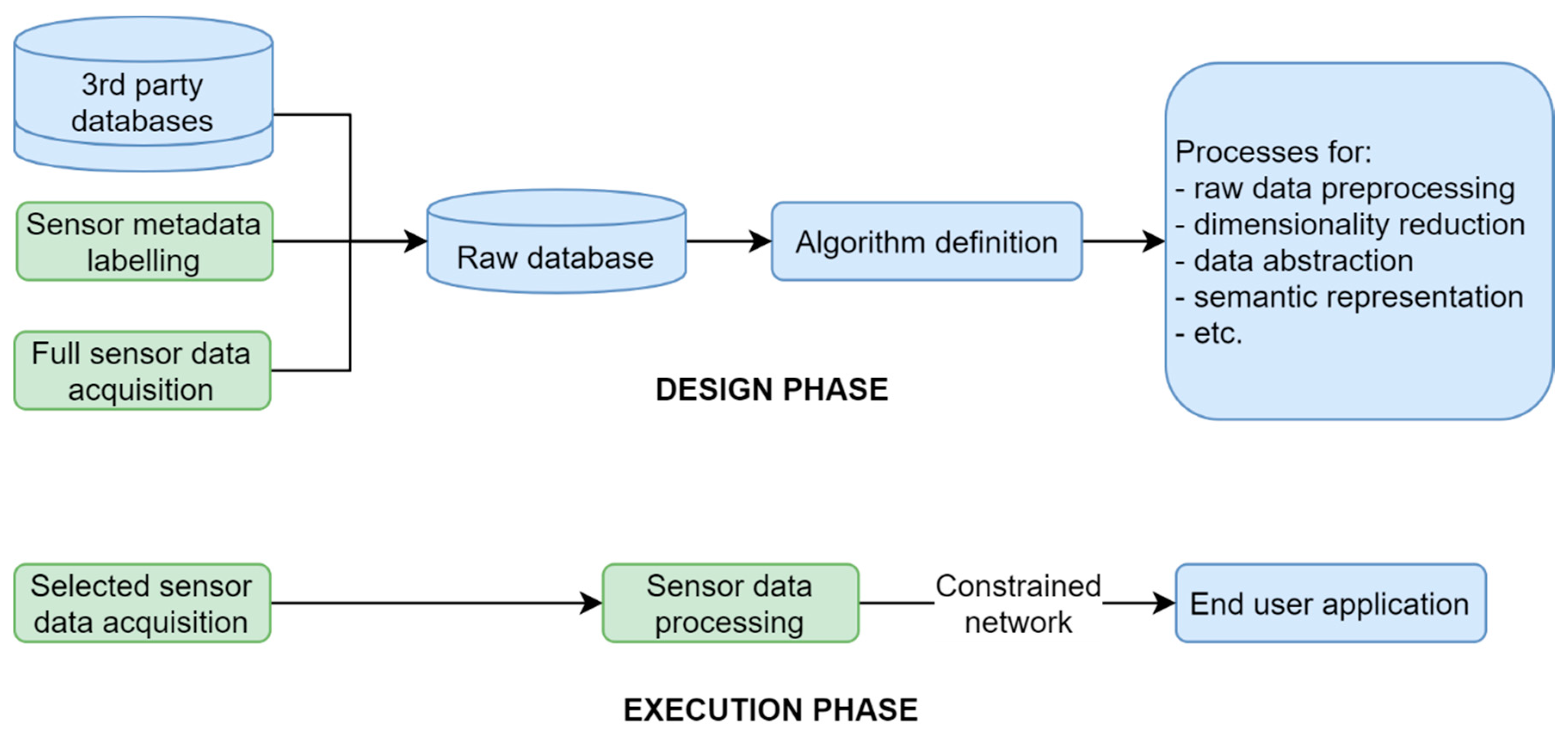
2. Materials and Methods

In this work, we analyse several VQ methods for reducing the dimensionality of raw data coming from inertial measuring unit (IMU) sensors while maintaining the highest quality of information. The aim of this study is to optimize the efficiency of a sensor equipped with an accelerometer, gyroscope, and magnetometer that monitors movement at 50 Hz so that it is capable of continuously sending this data to an external entity (e.g., the cloud) for analysis.

The smart sensor (Figure 4) consists of a Pycom’s Lopy4 module (Microprocessor ESP32 DualCore, 240 Mhz, RAM: 4 MB, ROM: 8 MB) and the inertial sensor BNO055 from Bosch. The device can communicate using different protocols depending on specific requirements: BLE/Wi-Fi/LoRa/Sigfox.

Considering a resolution of 16 bits at 50 Hz, sensor data are generated at about 300 bytes per second, which is a limitation in terms of the necessary energy and the data protocol used. According to Figure 1, wi-fi is used to send raw data in the design phase, and LoRa is used to send compressed data in the execution phase.

2.1. Data Processing Proposal

First, a public dataset must be chosen on which to apply the pre-processing and then the dimensionality-reduction or compression model. The objective is to validate the approach and quantify the errors produced for inertial sensors in different positions emitting different amounts of data. In addition, a labelled database is needed so that classifications can be made, if necessary. Then we will be able to evaluate the impact on the generalisation of the trained model with databases created by people outside the study and the chosen inertial sensors.

For this study, we analysed several public databases covering different human activities monitored using inertial sensors. Some databases involved a large number of activities [2,28], many test subjects [29], a large number of sensors [1], or a large amount of data [1,3,29]. In order to carry out an analysis of the compression model without involving a variety of activities [3] or the development of these activities [29], we chose the heterogeneity activity recognition dataset [1]. This database used inertial sensors in smartphones or smartwatches to record patterns in sitting, standing, walking, climbing stairs, descending stairs, and riding a bicycle. We analysed the repeatability and variability of the data from different devices in the database and finally chose the data from the Samsung S3 at a sampling frequency of 100 Hz. The Samsung S3 was positioned on the front of the torso with a belt.

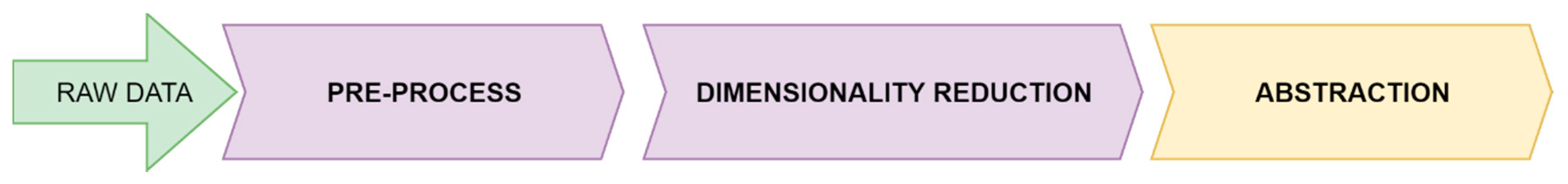
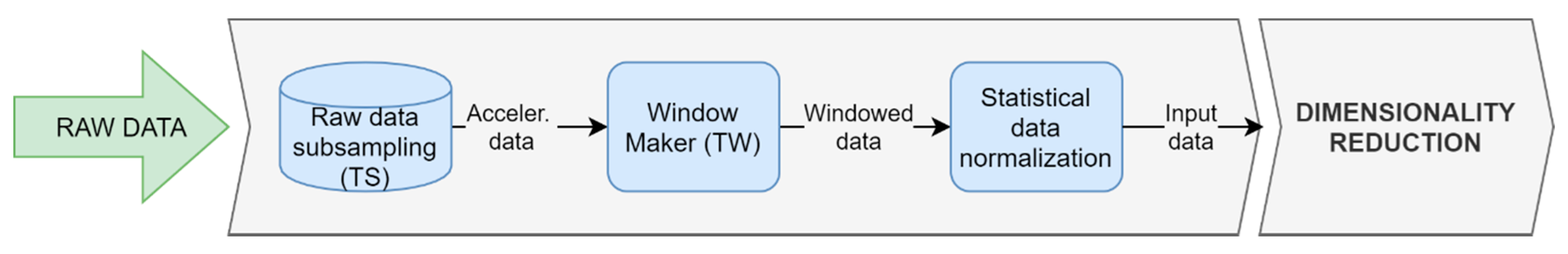
2.1.1. Data Pre-Processing

For the pre-processing of the data, we followed the steps indicated in Figure 5, which involved grouping sample sequences in data windows of variable sizes to evaluate their impact, as well as calculating statistical parameters to extract information from the dataset to provide to an abstraction layer.

• Raw data subsampling. In order to obtain more input data for training purposes, a subsampling option is included in the sensor sample rate (Tsoriginal) for the database. In this proposal, we considered three sampling frequencies: the original frequency, plus half-frequency subsampling, and quarter-frequency subsampling (Ts), producing two and four new signals, respectively, thus allowing us to increase the data collected.
• Window maker. There are two parameters that are used to define the window size (TW): the sensor sampling frequency (Ts) and the full sample time (Tf). To evaluate their impacts, different combinations have been tested, with the only restriction being that the window size must always be a natural number.
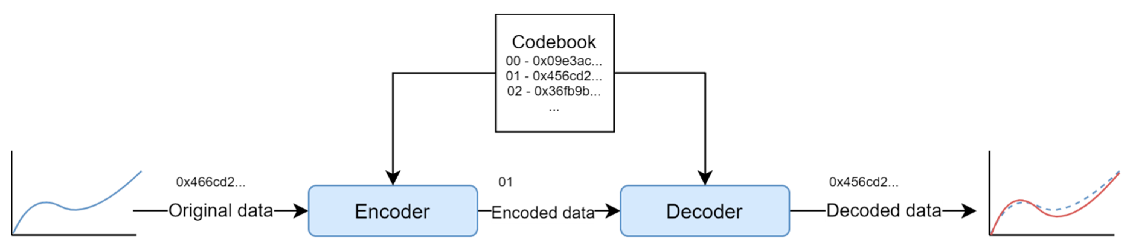
• Statistical data normalisation. Once the TW for the data window (x_i) is defined, it is standardized by subtracting its mean and dividing this quantity by its standard deviation, resulting in the standardized data window (x_i′) (see Equation (1)). The later data submission will include the mean value, the standard deviation, and the associated VQ index for (x_i′). Two additional VQs can be implemented to code the mean and standard deviation values, resulting in a data submission consisting of three fully encrypted indexes. However, for simplicity, in this work, only the standardized data vector is compressed.

$$x{’}_i=\frac{x_i-mean}{std}$$

(1)

Once all the tasks have been executed, the normalized data window, along with its average and standard deviation, will be available. The compressor model input will be the normalized window, which defines the expected input size. However, if the window calculation parameters are modified, it will be necessary to retrain the compressor model.

2.1.2. Dimensionality Reduction

The dimensionality reduction models analysed in this work are of the VQ type, a lossy compression technique that uses a competitive decision algorithm. To represent an input, the VQ selects a value from a list of indexes corresponding to the N-centroid table (codebook). Each input is a point in an n-dimensional space, where the set of N centroids is also located. The VQ divides this space by optimising the arrangement of the regions associated with each centroid, which are called Voronoi regions (Figure 6).

The usual VQ techniques, such as K-means, distribute the centroids by replicating the probability density of the occurrence of examples in that space. In this work, VQs based on MSCL (magnitude sensitive competitive learning) [26] will be applied, meaning that the arrangement of the centroids distributes equally among them a certain magnitude defined by a function local to the centroids.

In order to compare several compression objectives, three magnitude definitions will be analysed: fixed value, number of activations, and quantification error. When selecting a magnitude function with a constant value of one, the VQ generated is equivalent to a classical K-nearest neighbour (K-NN). When the magnitude counts the number of activations that a centroid has along its training cycles, the generated VQ is equivalent to the frequency sensitive competitive learning (FSCL) model [25], where the generated codebook optimizes the Shannon information entropy of the coding (in the optimal coding, the codes are used with uniform probability). For a magnitude that accounts for the mean quantification error (Qerror) of each centroid with the data it captures in its Voronoi region, this VQ, with error as magnitude, will be referred to as error sensitive competitive learning (ESCL).

The steps of the VQ training algorithm are shown in Algorithm 1. During training, the VQ recalculates the positions of the centroids by presenting the data set cyclically. Training stops when a certain error level for the obtained coding is met. In each cycle, each training example is assigned to one centroid based on a two-step competition. First, the BMU (best matching unit) and NMU (next matching unit) calculations are accomplished, obtaining the two centroids with the smallest Euclidean distances from the input data. Secondly, the LBMU (local best matching unit) calculation is performed to select the definitive winner among the two centroids, i.e., the centroid with the smallest product of its Euclidean distance with its local magnitude. Once all the training examples have been assigned to the centroids, we proceed to the update phase where new centroid positions are assigned. Next, if the local magnitude is not a fixed value, the algorithm selects the BMU for each training sample again using the updated codebook, and cumulates codebook-centroids wins and errors for updating their new magnitudes.

Algorithm 1. Adaptative VQ training

--- Perform initialization α0 = initial learning factor, αF = final learning factor, T = max training epoch, target_error = max error W = random(N, TW)--- Initial random codebook matrix W with N centroids of size TW Vmag = ones(N)--- Initial local magnitude vector Vmag for N centroids repeat--- training loop  Wupdate = zeros(N, TW) --- Init weight-updating matrix Wupdate  t = current training epoch  repeat --- codebook update loop  --- Compute quantification error Qerror for sample x:   Qerror[k] = (x − W[k, :])2  for k = 0, …, N – 1  --- Select Best Matching Unit:   BMU = argmin(Qerror)  --- Exclude BMU from Qerror list and select Next Matching Unit in the new list Qerror’:   Qerror’[k] = Qerror[k] for k = 0, …, N − 1  k ≠ BMU   NMU = argmin(Qerror’)  --- Select Local Best Matching Unit to the product of Qerror and Vmag among BMU and NMU:   LBMU = argmin(Vmag[BMU]*Qerror[BMU], Vmag[NMU]*Qerror[NMU])  --- Update weight-updating matrix for LBMU:   Wupdate[LBMU, :] += x − W[LBMU, :]  until end_of_data --- end of codebook update loop  --- Update learning factor α and codebook W:  α = α0 + (αF − α0) * sqrt(t/T)  W = W + α * Wupdate  --- Perform local magnitude update (only if local magnitude is ESCL or FSCL)  if magnitude is ESCL or magnitude is FSCL then   Vmag = zeros(N) --- Init centroids local magnitude vector   repeat --- local magnitude update loop   --- Compute sample error:    Qerror[k] = (x − W[k, :])2 k = 0, …, N − 1   --- Select Best Matching Unit:    BMU = argmin(Qerror)   --- Update local magnitude BMU:    if magnitude is ESCL then     Vmag[BMU] += Qerror[BMU] --- cumulate quantification error    else --- magnitude is FSCL     Vmag[BMU] += 1 --- cumulate centroid activation frequency    end if   until end_of_data --- end of local magnitude update loop  end if until error < target_error or t > T --- end of training loop

To choose the necessary function updating the local magnitude BMU, we must consider their different behaviours. The ESCL forces the VQ to form Voronoi regions with the same average error, so the centroids tend to present uniform quantification errors. The FSCL adjusts the Voronoi regions to obtain the same activation frequency, so the centroids are used with uniform probability. A unity magnitude adjusts the Voronoi regions to present the same data density, so the centroids tend to present uniform densities.

After training, the VQ will assign the winning centroid to an input (based on the Euclidean distance), so only the BMU calculation is applied. The output of the system will be the numerical index referring to that centroid.

2.2. Analysis of Method Performances

The performance evaluation of a compressor model is broken down into two phases; for each of them, a series of objectives and procedures is defined in order to verify the compression quality and the capacity of the running system.

Python 3 with the Pycharm IDE is used for the entire pre-processing and dimensionality reduction application. The smart sensor programming is done with MicroPython; thus, a large part of the generated code was reusable, except for the adaptation of certain libraries, including numpy.

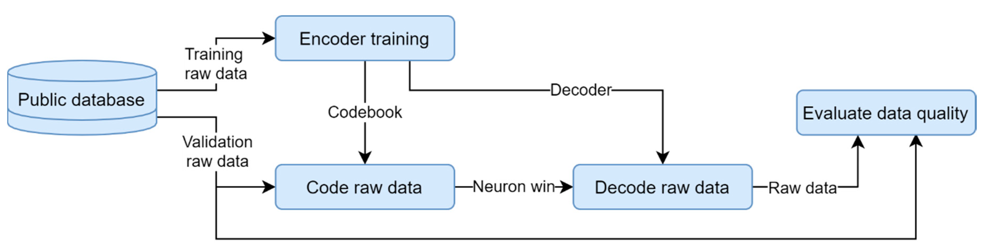
2.2.1. Offline Training and Run Validation

Once the codebook has been trained, the coding process calculates the Euclidean distance of each centroid from the data sample vector, and the closest centroid is determined. The winning centroid index will be transmitted as NeuronWin. Figure 7 shows the flow chart listing the steps taken in offline validation.

The decoding step consists of extracting the weights of the winning neuron from the centroid-weight lookup table as the data is reconstructed.

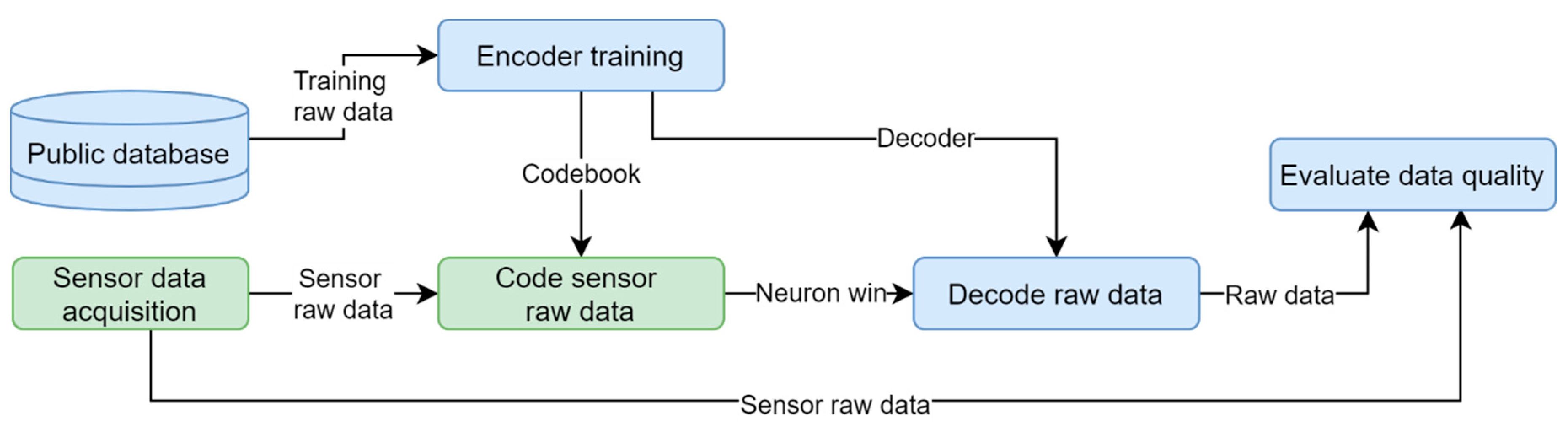
2.2.2. Offline Training and Online Run Validation

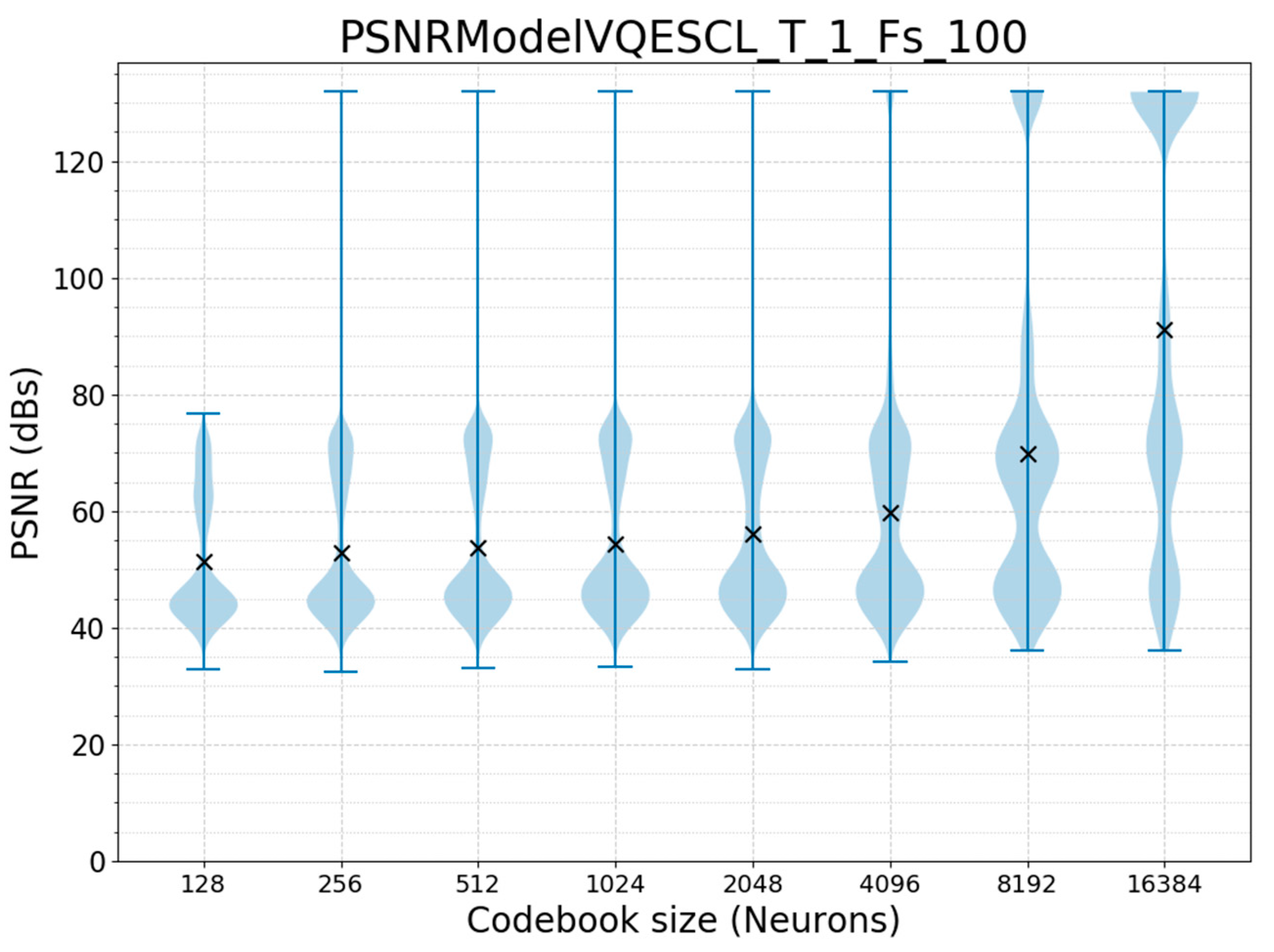
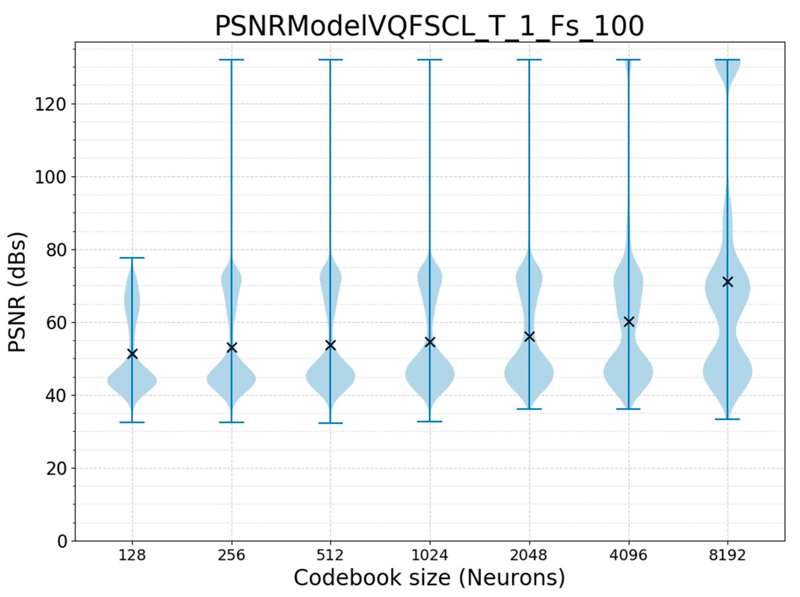
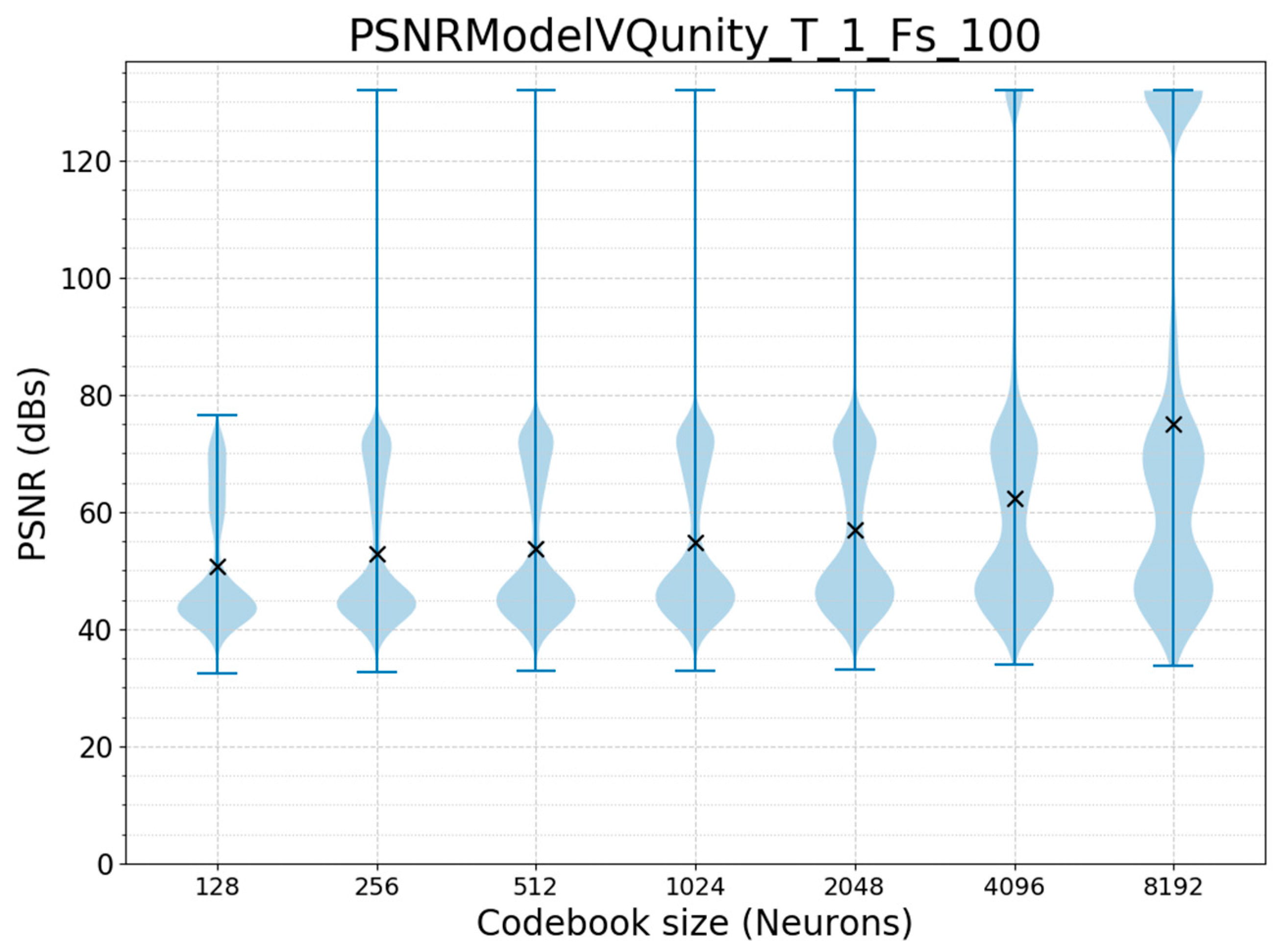
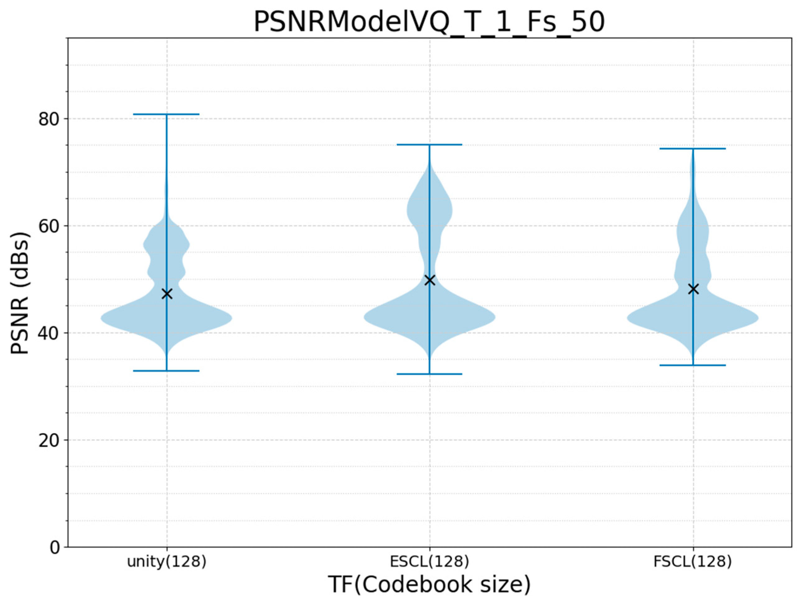
When verifying the model in the smart sensor itself, the aim is to: (i) evaluate the feasibility of implementing the compression system when the smart sensor is operating in real time, and (ii) measure the model generalisation of a compression designed offline with one set of data using different data.

The encoding process follows the same procedure as in the previous case with data from the sensor array Sensor raw data. Figure 8 describes the steps used to evaluate the adaptive model within the microcontroller and compare the error in the remote device.

The pre-processing and dimensionality-reduction models were incorporated into the microcontroller to encode the data from the inertial sensor. The size of the compressor model was designed with the microcontroller’s memory limitations in mind to allow for real-time implementation and operation. A wi-fi communication line was established between the device and the computer, allowing the computer to receive the raw data window, coded data, and statistical parameters. Once in the computer, we used the coded data to reconstruct the data (recovering the weights of the winning centroid used as a replacement for the original data) and evaluate the error committed in the compression.

3. Results

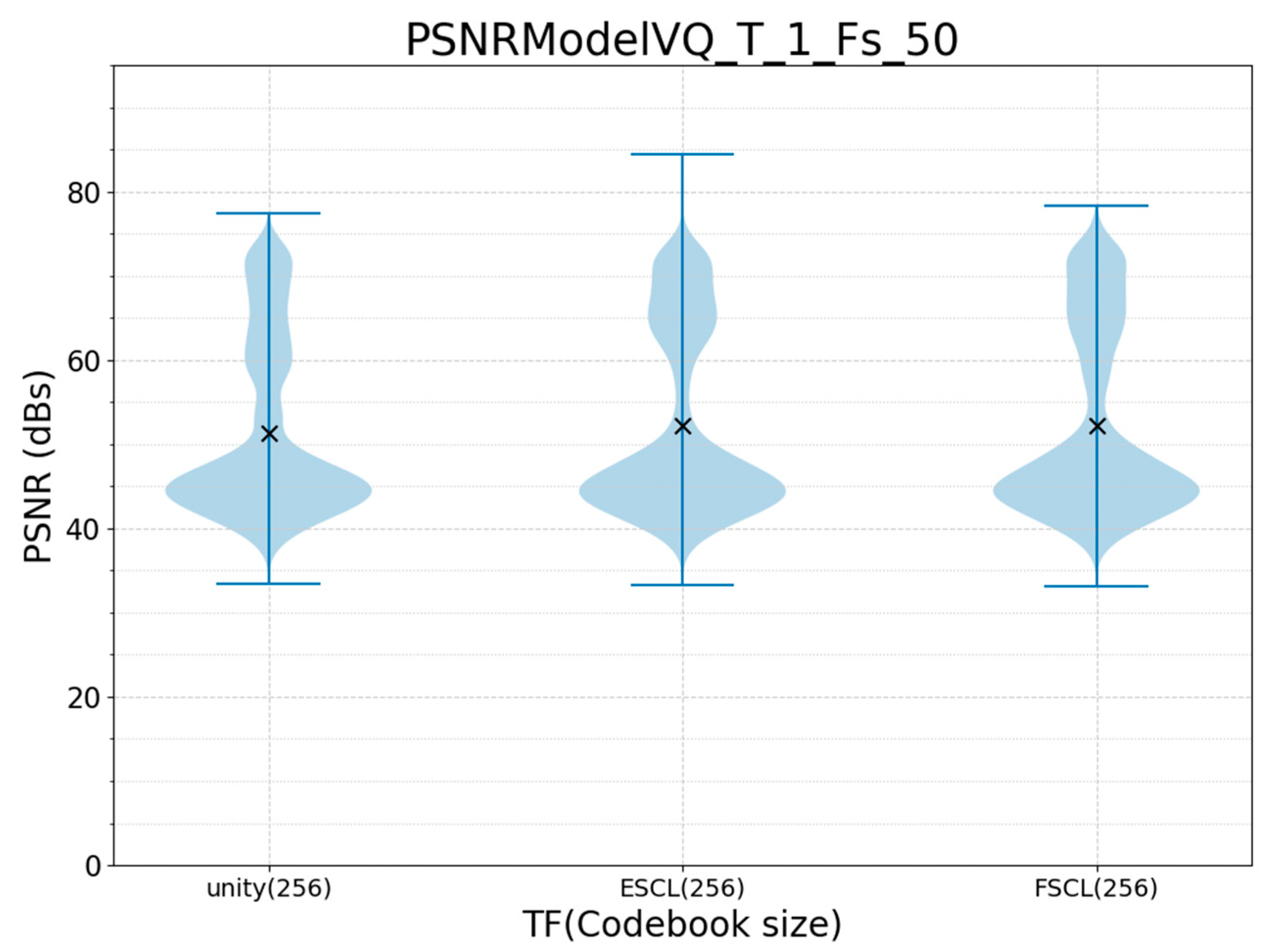
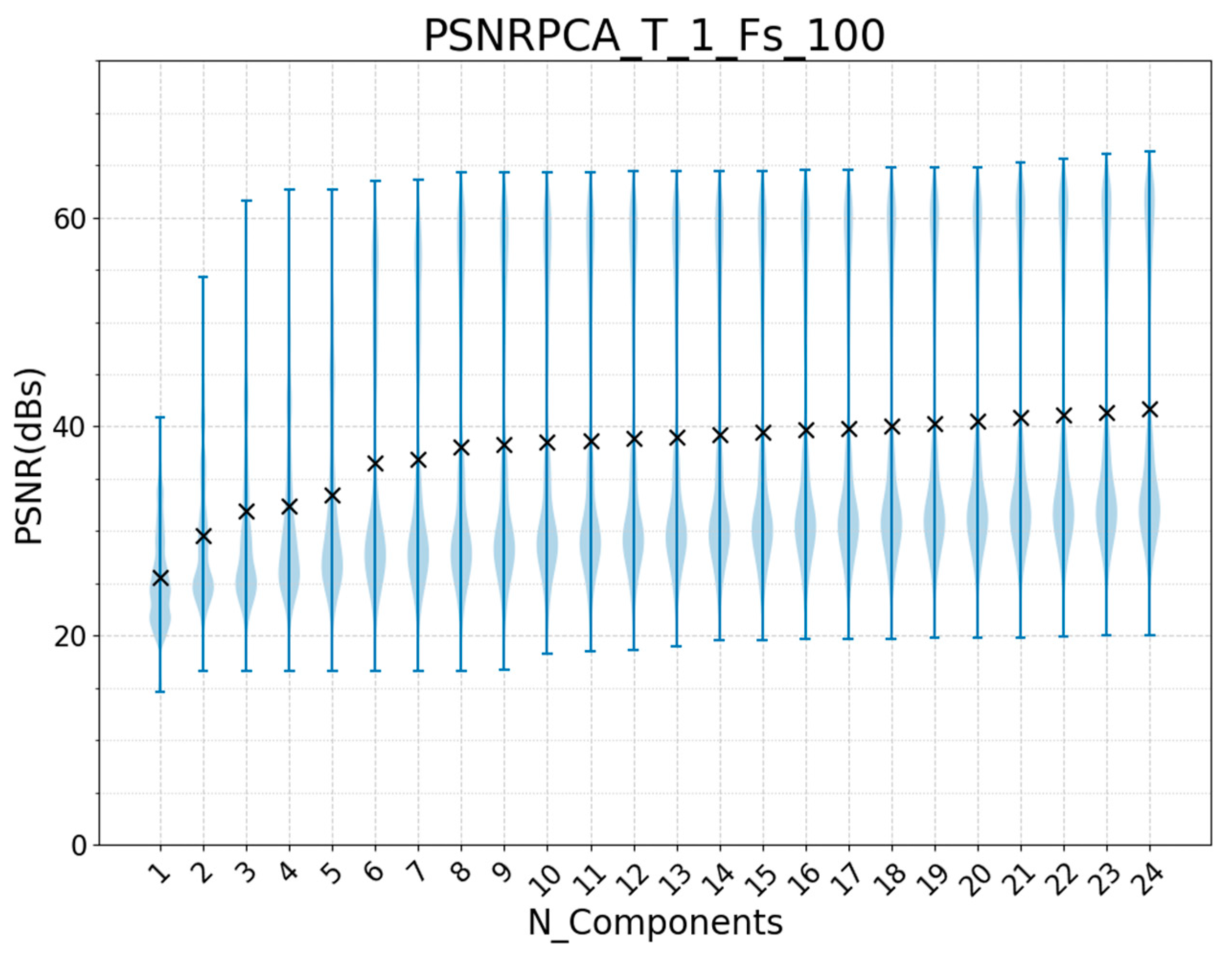
3.1. Offline Training and Run Validation

We evaluated different architectures by varying the sampling frequency (F), the size of the samples (T), and the number of centroids in the codebook (N). Of the raw data in the database, 1,961,400 samples were reserved for training, and 600,100 samples were used for testing. The model accuracy was measured with the mean squared error (MSE) when reconstructing the input signal. The peak signal-to-noise ratio (PSNR) measured the quality of that reconstruction. We also considered the size of the look-up table (LUT-Size) and the signal compression ratio (bits of the original signal vs. bits required for the codebook index, i.e., the compressed signal). Both parameters have a direct relationship with F, T, and N, and they must comply with the constraints imposed by the embedded system in terms of available memory and communication protocol.

Table 1. Evaluating temporal parameters F and T for the model (TF = FSCL, and N = 512).

Configuration				MSE_Train	Compression Rate	LUT-Size (kB)
F = 25 Hz	T = 0.6 s	N = 512	TF = FSCL	0.0320434	45	46.08
F = 50 Hz	T = 0.6 s	N = 512	TF = FSCL	0.0335083	90	92.16
F = 100 Hz	T = 0.6 s	N = 512	TF = FSCL	0.0351562	180	184.32
F = 25 Hz	T = 1 s	N = 512	TF = FSCL	0.0381469	75	76.8
F = 50 Hz	T = 1 s	N = 512	TF = FSCL	0.0406799	150	153.6
F = 100 Hz	T = 1 s	N = 512	TF = FSCL	0.0426330	300	307.2
F = 25 Hz	T = 1.6 s	N = 512	TF = FSCL	0.0445556	120	122.88
F = 50 Hz	T = 1.6 s	N = 512	TF = FSCL	0.0483703	140	245.76
F = 100 Hz	T = 1.6 s	N = 512	TF = FSCL	0.0509948	480	491.52

lists different combinations of the temporal parameters F and T for a fixed codebook size (N = 512), which allows us to visualize the compression level achieved and the required memory. In

Table 2. Evaluating the codebook size N for the model (TF = ESCL, F = 100 Hz and T = 1 s).

Configuration				MSE_Train	Compression Rate	LUT-Size (kB)
F = 100 Hz	T = 1 s	N = 128	TF = ESCL	0.049156436	600	76.8
F = 100 Hz	T = 1 s	N = 256	TF = ESCL	0.043934487	600	153.6
F = 100 Hz	T = 1 s	N = 512	TF = ESCL	0.039818928	300	307.2
F = 100 Hz	T = 1 s	N = 1024	TF = ESCL	0.036260296	300	614.4
F = 100 Hz	T = 1 s	N = 2048	TF = ESCL	0.03284163	300	1228.8
F = 100 Hz	T = 1 s	N = 4096	TF = ESCL	0.027240828	300	2457.6
F = 100 Hz	T = 1 s	N = 8192	TF = ESCL	0.019781198	300	4915.2

, the temporal parameters are set (F = 100 Hz, and T = 1 s) and different sizes for the codebook N are tested to show the effect on the MSE.

In Figure 9, Figure 10 and Figure 11, the PSNR distributions as well as the mean, minimum, and maximum values for the cases considered in Table 2. are shown while evaluating the three different target functions (ESCL, FSCL, and unity).

3.2. Offline Training and Online Run Validation

We have evaluated the suitability of the method using the models with N = 128 and N = 256 due to the memory constraints of the embedded system.

Table 3. Results for the embedded codification.

Configuration				PSNR_Mean	Compression Rate	LUT-Size (kB)
F = 50 Hz	T = 1 s	N = 128	TF = ESCL	49.83103058	300	38.4
F = 50 Hz	T = 1 s	N = 256	TF = ESCL	52.18381027	300	76.8
F = 100 Hz	T = 1 s	N = 128	TF = ESCL	51.46948697	600	76.8
F = 100 Hz	T = 1 s	N = 256	TF = ESCL	52.83481729	600	153.6

shows the PSNRs achieved by the embedded system for F = 50 Hz–100 Hz and N = 128–256. Figure 12 and Figure 13 show the PSNR distributions and mean, minimum, and maximum values obtained from evaluating the three different target functions (TF = ESCL, FSCL, unity).

Table 4. Results for generalising the embedded codification.

Configuration				PSNR_Mean	Compression Rate	LUT-Size (kB)
F = 50 Hz	T = 1 s	N = 128	TF = ESCL	41.10897725	300	38.4
F = 100 Hz	T = 1 s	N = 256	TF = ESCL	41.7319738	300	76.8

shows the PSNR achieved by the embedded system while using testing data instead of training data, which measures the generalisation of the model.

The PSNR for a PCA-based model up to 24 components has been calculated in order to compare it with the proposed VQ model (the number of components was set to reach 90% of the variance). It can be seen in Figure 14 how the average PSNR increases with the number of components, but it increases slowly when using more than 6 components, requiring at least 19 components to achieve the mean value of 40 dB, where each PCA component requires a 2-byte float16 data. This means that to obtain a value for an average PSNR between 40 and 50 dBs, we would have to use more than 19 components, which would be equivalent to 38 bytes, while VQ achieves similar or better PSNR figures, with only one byte being sent, leading to significative less data being transmitted.

4. Discussion

Compression rate is defined as the ratio between the size of the original signal and the compressed signal. In VQ compression methods it is established a priori when setting the model parameters F and T, which define the window size TW, and the number of bytes required to index a look-up table of size N. Thus, we can set the desired compression rate while considering the cost of the memory required to store the look-up table. We can see in Table 1 how the compression rate increases as the sampling frequency and sample size increase, i.e., as the LUT-Size does. Table 2 shows that the compression rate decreases when the number of neurons and the size of the look-up table increase, as we use two bytes to index codebooks with N > 256. Compression rate figures of 600 can be achieved in the smallest models with codebook sizes of 76.8 kB and 153.8 kB.

The MSE is related to the number of samples a single neuron in the codebook must represent. Table 1 shows that increasing the window size increases the MSE for a fixed number of neurons, while we can see in Table 2 how the MSE decreases as the number of neurons increases for a fixed window size. This same pattern can also be seen in Figure 9, Figure 10 and Figure 11, where the PSNR increases as the number of neurons N increases.

Looking at the PSNR distributions in Figure 9, Figure 10 and Figure 11, we can identify several regions of interest in these violin plots, namely, three regions between 80–40 dB, and a fourth region in the highest part of the chart above 120 dB, which appears only in models with the highest number of neurons. This region corresponds to a nearly perfect reconstruction where the centroid weights have hardly any noise, thus indicating an overfitting performance, where single centroids dedicated to code individual samples appear. To avoid this situation, codebook sizes must be at least 5–10 times smaller than the number of samples to learn in order to force the centroids to learn different patterns. Next, an area between 80–60 dB corresponds to small Voronoi regions where low noise for the reconstructed signal can be found and is more evident in models with higher numbers of neurons. Between 60–50 dB, we can observe a neck belonging to the intermediate-sized Voronoi regions, in which certain signals are close to the centroid, but other signals appear on the periphery of the Voronoi region, giving rise to lower PSNR values. Lastly, in the 50–40 dB area, the Voronoi regions are large and, as they comprise widely separated input data values, they produce situations with noisier reconstructions.

In Figure 9, an extra simulation with 16,384 neurons is added, in which we can see a greater growth in the neurons capable of nearly replicating the pattern exactly, as well as an increase in the average. This situation is due to the fact that the number of neurons is very large and the centroids have few examples to train, so they adjust to replicate the input values.

We can see a large increase in the mean from N = 4096 to N = 8192, as well as the appearance of overfitting in the 120 dB zone in the violin plot. As the objective is to achieve high compression, we will focus on the area from N = 128 to N = 1024, in which the evolution of the model is clear. We can see in the evolution of the 60–40 dB and 60–80 dB areas how, as we add more neurons, the data goes towards areas with higher PSNR values, increasing the density in the area by approximately 70 dB. With this model, we achieve a good balance by obtaining PSNR values greater than 50 dB while applying compression factors greater than 300.

In Figure 12 and Figure 13, two models are selected to analyse the impact of the target function used. If we look at Figure 12, the ESCL model gives the best response. The average in this model is higher than those in the other two, and the 50–70 dB zone is wider than it is in the other two, providing a better compression result. Figure 13 produces a similar result but with a less pronounced difference, as the number of centroids is duplicated. In both model parametrisations, the FSCL and unity magnitudes tend to be similar. This effect tends to occur when the distribution of data points is almost uniform, making the density and frequency of activation essentially equivalent.

The implementation of the microcontroller compression algorithm shows the importance of establishing an adequate map size to limit the embedded system when applying the models at N = 128 to get the system working properly.

In Table 3, we verify the correct implementation of the algorithm in the embedded device, allowing the signal to compress in the same way that it does in the offline process. For this implementation, models such as those that appear in Table 1 have been evaluated, achieving similar results. The generalisation of the model evaluation results in Table 4 shows how the PSNR has decreased compared to the values obtained in Table 3, as expected. However, the PSNR remains at values above 40 dB.

5. Conclusions

We are surrounded by sensors that collect data from the environment continuously and send them to the Internet. Reductions in their data rates are necessary in order to enhance their energy usage, improve data security, and minimize the sensor data traffic generated by billions of IoT devices.

In an implementation of VQ models, we define an adaptative codebook that evolves to become highly specific to the input data. It has been designed to look for a balance between complexity (allowing implementation in embedded devices) and error minimisation. We found that the ESCL model was the best VQ algorithm, as it was able to provide compression factors between 300 and 600 with PSNR values varying from 40 dB to 70 dB.

This work provides evidence that VQ methods are able to reduce the dimensionality of raw data within an embedded device, with the memory required for their adaptive look-up tables being their main limitation. The use of additional external flash memory could allow the use of larger look-up tables and improve performance. An additional benefit of VQ encoding is that data encryption is possible in situations where the data to be transmitted could be intercepted [30]. At very low energy costs, VQ encoding makes it nearly impossible to decode the data sent in the absence of a model.

References

1. Stisen, A.; Blunck, H.; Bhattacharya, S.; Prentow, T.S.; Kjaergaard, M.B.; Dey, A.; Sonne, T.; Jensen, M.M. Smart devices are different: Assessing and mitigatingmobile sensing heterogeneities for activity recognition. In Proceedings of the 13th ACM Conference on Embedded Networked Sensor Systems, Seoul, Korea, 1–4 November 2015; ACM: New York, NY, USA, 2015; pp. 127–140. [Google Scholar]
2. Banos, O.; Moral-Munoz, J.; Diaz-Reyes, I.; Arroyo-Morales, M.; Damas, M.; Herrera-Viedma, E.; Hong, C.S.; Lee, S.; Pomares, H.; Rojas, I.; et al. mDurance: A Novel Mobile Health System to Support Trunk Endurance Assessment. Sensors 2015, 15, 13159–13183. [Google Scholar] [PubMed] [Green Version]
3. Banos, O.; Villalonga, C.; Garcia, R.; Saez, A.; Damas, M.; Holgado, J.A.; Lee, S.; Pomares, H.; Rojas, I. Design, implementation and validation of a novel open framework for agile development of mobile health applications. Biomed. Eng. Online 2015, 14, 1–20. [Google Scholar] [CrossRef] [PubMed] [Green Version]
4. Ganz, F.; Puschmann, D.; Barnaghi, P.; Carrez, F. A Practical Evaluation of Information Processing and Abstraction Techniques for the Internet of Things. IEEE Internet Things J. 2015, 2, 340–354. [Google Scholar] [CrossRef] [Green Version]
5. Prasertsung, P.; Horanont, T. A classification of accelerometer data to differentiate pedestrian state. In Proceedings of the 2016 International Computer Science and Engineering Conference (ICSEC), Chiang Mai, Thailand, 14–17 December 2016; pp. 1–5. [Google Scholar]
6. Noor, M.; Salcic, Z.; Wang, K. Adaptive sliding window segmentation for physical activity recognition using a single tri-axial accelerometer. Pervasive Mob. Comput. 2017, 38, 41–59. [Google Scholar] [CrossRef]
7. Banos, O.; Galvez, J.; Damas, M.; Pomares, H.; Rojas, I. Window Size Impact in Human Activity Recognition. Sensors 2014, 14, 6474–6499. [Google Scholar] [CrossRef] [Green Version]
8. Krishnan, N.C.; Panchanathan, S. Analysis of low resolution accelerometer data for continuous human activity recognition. In Proceedings of the 2008 IEEE International Conference on Acoustics, Speech and Signal Processing, Las Vegas, NV, USA, 31 March–4 April 2008; pp. 3337–3340. [Google Scholar]
9. Marqués, G.; Basterretxea, K. Efficient algorithms for accelerometer-based wearable hand gesture recognition systems. In Proceedings of the 2015 IEEE 13th International Conference on Embedded and Ubiquitous Computing, Porto, Portugal, 21–23 October 2015; pp. 132–139. [Google Scholar]
10. Sukor, A.S.A.; Zakaria, A.; Rahim, N.A. Activity recognition using accelerometer sensor and machine learning classifiers. In Proceedings of the 2018 IEEE 14th International Colloquium on Signal Processing & Its Applications (CSPA), Batu Feringghi, Malaysia, 9–10 March 2018; pp. 233–238. [Google Scholar]
11. Jahanjoo, A.; Tahan, M.N.; Rashti, M.J. Accurate fall detection using 3-axis accelerometer sensor and MLF algorithm. In Proceedings of the 2017 3rd International Conference on Pattern Recognition and Image Analysis (IPRIA), Shahrekord, Iran, 19–20 April 2017; pp. 90–95. [Google Scholar]
12. Sancheti, P.; Shedge, R.; Pulgam, N. Word-IPCA: An improvement in dimension reduction techniques. In Proceedings of the 2018 International Conference on Control, Power, Communication and Computing Technologies (ICCPCCT), Kannur, India, 23–24 March 2018; pp. 575–578. [Google Scholar]
13. Padmaja, D.L.; Vishnuvardhan, B. Comparative study of feature subset selection methods for dimensionality reduction on scientific data. In Proceedings of the 2016 IEEE 6th International Conference on Advanced Computing (IACC), Bhimavaram, India, 27–28 February 2016; pp. 31–34. [Google Scholar]
14. Dua, Y.; Kumar, V.; Singh, R. Comprehensive review of hyperspectral image compression algorithms. Opt. Eng. 2020, 59. [Google Scholar] [CrossRef]
15. Sustika, R.; Sugiarto, B. Compressive Sensing Algorithm for Data Compression on Weather Monitoring System. TELKOMNIKA Telecommun. Comput. Electron. Control 2016, 14, 974. [Google Scholar] [CrossRef] [Green Version]
16. Moon, A.; Kim, J.; Zhang, J.; Son, S.W. Lossy compression on IoT big data by exploiting spatiotemporal correlation. In Proceedings of the 2017 IEEE High. Performance Extreme Computing Conference (HPEC), Waltham, MA, USA, 12–14 September 2017; pp. 1–7. [Google Scholar]
17. Fragkiadakis, A.; Charalampidis, P.; Tragos, E. Adaptive compressive sensing for energy efficient smart objects in IoT applications. In Proceedings of the 2014 4th International Conference on Wireless Communications, Vehicular Technology, Information Theory and Aerospace & Electronic Systems (VITAE), Aalborg, Denmark, 11–14 May 2014; pp. 1–5. [Google Scholar]
18. Deepu, C.; Heng, C.; Lian, Y. A Hybrid Data Compression Scheme for Power Reduction in Wireless Sensors for IoT. IEEE Trans. Biomed. Circuits Syst. 2017, 11, 245–254. [Google Scholar] [CrossRef] [PubMed]
19. Azar, J.; Makhoul, A.; Barhamgi, M.; Couturier, R. An energy efficient IoT data compression approach for edge machine learning. Future Gener. Comput. Syst. 2019, 96, 168–175. [Google Scholar] [CrossRef] [Green Version]
20. Razzaque, M.; Bleakley, C.; Dobson, S. Compression in wireless sensor networks. ACM Trans. Sens. Netw. 2013, 10, 1–44. [Google Scholar] [CrossRef]
21. Stojkoska, B.R.; Nikolovski, Z. Data compression for energy efficient IoT solutions. In Proceedings of the 2017 25th Telecommunication Forum (TELFOR), Belgrade, Serbia, 21–22 November 2017; pp. 1–4. [Google Scholar]
22. M, L.; Sarvagya, M. MICCS: A Novel Framework for Medical Image Compression Using Compressive Sensing. Int. J. Electr. Comput. Eng. 2018, 8, 2818. [Google Scholar] [CrossRef]
23. Ayoobkhan, M.; Chikkannan, E.; Ramakrishnan, K. Lossy image compression based on prediction error and vector quantisation. EURASIP J. Image Video Process. 2017, 2017, 35. [Google Scholar] [CrossRef] [Green Version]
24. Choudhury, S.; Bandyopadhyay, S.; Mukhopadhyay, S.; Mukherjee, S. Vector quantization and multi class support vector machines based fingerprint classification. In Proceedings of the 2016 International Conference on Inventive Computation Technologies (ICICT), Coimbatore, India, 26–27 August 2016; Volume 2, pp. 1–4. [Google Scholar]
25. Banerjee, A.; Ghosh, J. Frequency-sensitive competitive learning for scalable balanced clustering on high-dimensional hyperspheres. IEEE Trans. Neural Netw. 2004, 15, 702–719. [Google Scholar] [CrossRef] [PubMed]
26. Pelayo, E.; Buldain, D.; Orrite, C. Magnitude Sensitive Competitive Learning. Neurocomputing 2013, 112, 4–18. [Google Scholar] [CrossRef]
27. Lee, S.M.; Yoon, S.M.; Cho, H. Human activity recognition from accelerometer data using convolutional neural network. In Proceedings of the 2017 IEEE International Conference on Big Data and Smart Computing (BigComp), Jeju, Korea, 13–16 February 2017; pp. 131–134. [Google Scholar]
28. Altun, K.; Barshan, B. Human activity recognition using inertial/magnetic sensor units. In Human Behavior Understanding; Springer: Berlin/Heidelberg, Germany, 2010. [Google Scholar]
29. Casale, P.; Pujol, O.; Radeva, P. Personalization and user verification in wearable systems using biometric walking patterns. Per. Ubiquitous Comput. 2012, 16, 560–580. [Google Scholar] [CrossRef]
30. Healy, M.; Newe, T.; Lewis, E. Security for wireless sensor networks: A review. In Proceedings of the 2009 IEEE Sensors Applications Symposium, New Orleans, LA, USA, 17–19 February 2009; pp. 80–85. [Google Scholar]
Figure 1. Data constraints in the design and execution phases.
Electronics 09 02035 g001
Figure 2. Data compression—abstraction process [4].
Electronics 09 02035 g002
Figure 3. Vector quantisation compression.
Electronics 09 02035 g003
Figure 4. Smart sensor and cloud block diagram.
Electronics 09 02035 g004
Figure 5. Pre-processing tasks applied to the dataset.
Electronics 09 02035 g005
Figure 6. Example of Voronoi regions and their associated centroids (points).
Electronics 09 02035 g006
Figure 7. Offline compressor model validation.
Electronics 09 02035 g007
Figure 8. Online (blue) and offline (green) compressor model validation.
Electronics 09 02035 g008
Figure 9. Peak signal-to-noise ratio (PSNR) distribution and mean value (x) vs. codebook size N for the error sensitive competitive learning (ESCL) model (F = 100 Hz, T = 1 s).
Electronics 09 02035 g009
Figure 10. PSNR distribution and mean value (x) vs. codebook size N for the frequency sensitive competitive learning (FSCL) model (F = 100 Hz, T = 1 s).
Electronics 09 02035 g010
Figure 11. PSNR distribution and mean value (x) vs. codebook size N for the unity model (F = 100 Hz, T = 1 s).
Electronics 09 02035 g011
Figure 12. PSNR distribution and mean value (x) vs. the target function (F = 50 Hz, T = 1 s, N = 128).
Electronics 09 02035 g012
Figure 13. PSNR distribution and mean value (x) vs. the target function (F = 50 Hz, T = 1 s, N = 256).
Electronics 09 02035 g013
Figure 14. PSNR distribution and mean value (x) vs. number of components for PCA.
Electronics 09 02035 g014