V2I Propagation Loss Predictions in Simplified Urban Environment: A Two-Way Parabolic Equation Approach

Abstract

This study is devoted to radio wave propagation modeling in the urban environment. Special attention has been paid to the features of vehicular ad hoc networks (VANETs) and vehicle-to-infrastructure (V2I) communications. For the first time, the three-dimensional bidirectional parabolic equation (PE) method has been applied to the specified problem. Buildings and other obstacles are modeled by impenetrable (perfectly electric conducting) cuboids. A harmonic radiation source with an arbitrary direction pattern may be modeled. Numerical simulation is performed for various propagation scenarios. A comparison with the ray-tracing (RT) method is given. The results of the numerical simulation prove the effectiveness and reliability of the proposed method. Some recommendations for deploying VANETs are obtained based on the numerical results.

1. Introduction

Many studies are currently being conducted on the development, deployment, and operation of vehicular ad hoc networks (VANETs) [1,2,3]. It is expected that such networks will contribute to road safety, effective management of automobile traffic, development of driver assistance systems and autonomous vehicles. This technology is based on the communion of vehicles over a wireless communication channel with each other, fixed base stations and pedestrians. Vehicular communication systems follow the IEEE 802.11p standard, operating at 5.9 GHz.

With the increasing density of transmitting radio devices, the problem of their optimal location is becoming more acute. It is necessary to increase its real coverage and reduce mutual interference. Vehicular communications are characterized by quite complex conditions for radio wave propagation. Such systems are usually deployed in urban areas with dense automobile and pedestrian traffic [4]. Effective deployment of VANETs in urban environments requires a clear understanding of the impact of various propagation effects, as well as the ability to model them depending on specific conditions. In addition, it is necessary to take into account the parameters of the source and receiver, its antennas, and restrictions related to electromagnetic compatibility and sanitary standards. Unlike most of the tropospheric radio wave propagation problems, urban propagation is essentially three-dimensional. The source and receiver are located close to the ground, at an altitude of only a few meters. Propagation is greatly affected by buildings, cars, vegetation, pedestrians, and other urban obstacles. All the variety of wave propagation effects, such as interference, diffraction, scattering, reflection, and refraction, are observed simultaneously. All this reasons create high demands for the corresponding wave propagation models. Propagation models should be essentially site-specific. So effective propagation modeling requires knowledge of the terrain profile and the location of buildings.

All existing urban wave propagation models can be roughly divided into two categories: empirical and deterministic [5]. Empirical models are more widely used because of their simplicity [6]. They are based on a statistical analysis of experimental data and some empirical considerations. Based on them, it is relatively easy to implement computational programs for getting a quick solution to the problem. However, the resulting solutions are only estimates and do not always have sufficient accuracy. In addition, each specific empirical model has rather narrow limits of applicability. Therefore, it is usually necessary to develop new empirical models for each new communication system. Empirical models and measurements are used to study the propagation losses between moving cars in the urban environment [7,8]. Similar research has been conducted for the vehicle-to-infrastructure (V2I) scenario [9]. The default approach to radio coverage prediction is to use the recommendations of the International Telecommunication Union [10], which are based on empirical models. A comprehensive overview of the millimeter-waves propagation models is given in [11].

On the other hand, deterministic methods have rather wide limits of applicability. They can be used under urban, suburban, and rural scenarios for various frequency ranges without significant modifications. The most rigorous of the widely used methods for calculating losses in the urban environment is the 3D ray-tracing (RT) method [12]. It is based on geometric optics and the geometric theory of diffraction. The RT method allows one to model obstacles of an arbitrary geometric shape and size. It is also well adapted to account for complex boundary conditions on the obstacle surface. The advantages of the RT method also include the interpretability of the computation results. The RT method is used in indoor [13], outdoor [14] and outdoor-to-indoor [15] propagation scenarios. There are several studies [16,17] dedicated to the application of the RT method to V2I radio channel modeling in urban areas. A good agreement was obtained with the experimental data. The influence of automobile traffic using the RT method is investigated in [18].

The calculation of propagation by deterministic methods is usually much time and memory consuming than by empirical ones. However, with the growth of the processor’s performance and cloud computing, this argument is gradually losing its relevance. In addition, deterministic methods are useful for calibration and verification of the empirical ones [19], since it is not always possible to provide full-scale measurement campaigns.

In this paper, we propose to use the rigorous parabolic equation (PE) method [20], which is based on Maxwell’s equations. This method is widely used for solving problems of long-range propagation in tropospheric waveguides [21,22]. Although the PE method is usually used in a two-dimensional inhomogeneous environment, there are a number of papers devoted to its application in essentially three-dimensional problems. Application of the vector PE to modeling diffraction on buildings is discussed in [23,24]. Calculation of scattering from cars on the motorway using the PE method is considered in [25]. The PE method is used to calculate the field in tunnels [26].

The aim of this work is to prove the possibility of effective use of the three-dimensional bidirectional PE method in the radio wave propagation problem in dense urban development. When setting the problem and providing the numerical results, special attention has been paid to the above-mentioned features of VANET and V2I communications. This paper does not consider the influence of complex boundary conditions and Fresnel reflections [27]. Obstacles are modeled by impenetrable cuboids. Time variances and signal delays are also out of consideration. Keeping in mind the made simplifications of the environment, the real-world application of the obtained results is quite limited.

The paper is organized as follows. In the next section, we analyze the requirements for propagation models that arise from the specifics of VANET and pose the research task. Section 3 is devoted to the theoretical analysis of the proposed two-way 3D PE method. Numerical examples and comparison with the RT method are given in Section 4.

2. Problem Statement

In this paper, we proceed from the IEEE 802.11p standard and the operation frequency of 5900 MHz. We calculate propagation losses from a stationary located VANET base station to potential receivers on the vehicles. The base station is equipped with a vertically polarized dipole antenna and is located at a height of 2–5 m. It is assumed that the receiving antenna is located on the roof of the car at a height of about 1.5 m. Based on the average values for the corresponding equipment and sanitary standards, we further assume that the source power is 27 dBm, and the minimum threshold of the received signal is −96 dBm.

Interaction with the Earth’s surface, buildings, and cars will be taken into account. In this research, we restrict ourselves to the case of perfectly electric conducting (PEC) impediment boundaries.

The input data of the method under development are the radiation pattern and the height of the transmitting antenna, the location and geometric shape of buildings, cars and other obstacles. In this study, all obstacles are modeled by PEC cuboids. We are seeking a three-dimensional distribution of the received signal level.

3. 3D Parabolic Equation Method

The main advantage of the PE method is that it is directly derived from Maxwell’s equations [20]. This potentially allows it to take into account the vector nature of electromagnetic fields and depolarization effects. Unlike the RT method, the PE does not require separate consideration of diffraction, scattering, reflection, and refraction. These effects are already present in the original equation and are taken into account automatically. The only exception is backscattering, which is taken into account using the iterative procedure described below. The disadvantage of the PE method is the computational time and the relative complexity of the software implementation since rather non-trivial numerical methods are used.

Initially, the PE method was a narrow-angle approximation [28]. Currently, the limit on the maximum propagation angle is removed and modern modifications of the PE method allows calculating the field for any propagation angles [20,29], provided that a sufficiently dense computational grid is selected. The optimal selection of the computational parameters for the PE method is discussed in [29].

In this research, we consider a harmonic signal source, although there are works devoted to the application of the PE method in the time domain [30].

3.1. Derivation

Next, we assume a harmonic dependence of the form $exp(-i\omega t)$. The solution is seeking in the Cartesian coordinate system. Using the vector electric and magnetic Hertz potentials (${\Pi }^e$ and ${\Pi }^m$), the original Maxwell equations may be written as follows [31]

$$\Delta {\Pi }^e+k^2{\Pi }^e=\delta \left(x\right)\delta \left(y\right)f^e\left(z\right){\mathbf{e}}_z,$$

(1)

$$\Delta {\Pi }^m+k^2{\Pi }^m=0,$$

where $k=2\pi /\lambda$ is the wavenumber, $\lambda$ is the wave length, $\delta (·)$ is the Dirac delta function, ${\mathbf{e}}_z=(0,0,1)$. The function on the right-hand side of Equation (1) is responsible for the radiating source modeling. In our case, the source is omnidirectional in the horizontal plane and has a direction in the vertical plane. The radiation pattern in the vertical plane is modeled by function $f^e\left(z\right)$.

We set the Dirichlet condition on vertical surfaces (walls of buildings) [23]

$${\Pi }_z^e=0,$$

and the Neumann condition on horizontal surfaces (ground surface and roofs)

$$\frac{\partial {\Pi }_z^e}{\partial n}=0.$$

Depolarization effects can be ignored for the selected problem geometry and boundary conditions. Thus, further in this paper we can limit ourselves to considering the scalar three-dimensional Helmholtz equation

$$\frac{{\partial }^2\psi }{\partial x^2}+\frac{{\partial }^2\psi }{\partial y^2}+\frac{{\partial }^2\psi }{\partial z^2}+k^2\psi =0,$$

$$\psi \left(x,y,z\right)={\Pi }_z^e\left(x,y,z\right).$$

To remove factor $exp\left(ikx\right)$, we take into consideration a new function

$$u(x,y,z)=exp(-ikx)\psi (x,y,z).$$

The waves traveling in a positive x-direction are subject to the following equation [20]

$$\frac{\partial u}{\partial x}=ik(\sqrt{1+L}-1)u,$$

(2)

$$Lu=\frac{1}{k^2}\frac{{\partial }^{2}u}{\partial y^2}+\frac{1}{k^2}\frac{{\partial }^{2}u}{\partial z^2}.$$

Step-by-step solution of (2) can be written using the propagation operator $\mathbf{P}$ as follows

$$u(x+\Delta x,z)=exp\left(ik\Delta x\left(\sqrt{1+L}-1\right)\right)u(x,z)=\mathbf{P}u(x,z).$$

(3)

The wave field is generated by the initial condition

$$\psi (0,z)=f^e\left(z\right).$$

3.2. Split-Step Fourier Numerical Method

There are two most commonly used numerical methods for solving PE (2): split-step Fourier method (SSF) [32,33] and finite-difference (FD) approximations [21,34]. Both methods have their pros and cons [35,36]. FD methods are well suited for complex boundary conditions modeling, but so far they are inferior to the SSF method in performance, especially in the three-dimensional case. Since accounting for the complex boundary conditions is beyond the scope of this paper we further use the SSF method.

All existing numerical methods for solving PE are step-by-step with respect to the variable x. We use a uniform computational grid with a step $\Delta x$ by the longitudinal coordinate x and $\Delta y$, $\Delta z$ by the transversal coordinates y and z.

Using the definition of a pseudodifferential operator via the Fourier transform [37], propagation operator (3) takes the form

$$u(x+\Delta x,y,z)=\frac{1}{2\pi }\underset{-\infty }{\overset{+\infty }{\int }}\underset{-\infty }{\overset{+\infty }{\int }}exp\left(i{k}_{y}y+i{k}_{z}z\right)exp\left(ik\Delta x\left(\sqrt{1-\frac{k_y^2}{k^2}-\frac{k_z^2}{k^2}}-1\right)\right)\tilde{u}(x,k_y,k_z)d{k}_{y}d{k}_z,$$

(4)

$$\tilde{u}(x,k_y,k_z)=\frac{1}{2\pi }\underset{-\infty }{\overset{+\infty }{\int }}\underset{-\infty }{\overset{+\infty }{\int }}u(x,y,z)exp(-i{k}_{y}y-i{k}_{z}z)dydz.$$

(5)

For numerical calculation of integrals (4) and (5) we introduce the following uniform grid in the spatial and spectral domains

$$y_s=2y_{max}\left(s-\frac{n_y}{2}\right),s=0...n_y-1,$$

$$z_t=2z_{max}\left(t-\frac{n_z}{2}\right),t=0...n_z-1,$$

$$k_{y,s}=\frac{\pi }{y_{max}}\left(s-\frac{n_y}{2}\right),s=0...n_y-1,$$

$$k_{z,t}=\frac{\pi }{z_{max}}\left(t-\frac{n_z}{2}\right),t=0...n_z-1.$$

Two-dimensional Fourier transform (5) is approximated as follows [38]

$$\tilde{u}(x,k_{y,s},k_{z,t})\approx {(-1)}^{t+s}\frac{\Delta y\Delta z}{2\pi }\mathrm{FFT}2\left[{(-1)}^{p+q}u(x,y_p,z_q)\right],$$

where $\mathrm{FFT}2$ is the two-dimensional discrete Fourier transform operator. Negative z values are used for ground boundary modeling. Integral (4) is calculated in the same way.

The numerical solution of the problem is sought in an unbounded domain. The method of artificial absorbing layer is used to model transparent boundaries of the finite computational domain [23].

In contrast to other widely used computational electromagnetic methods, such as finite difference time domain method or method of moments [39], the PE method allows using sufficiently large grid steps. Namely, the longitudinal grid step $\Delta x$ may be taken equal to hundreds of wavelengths. Transversal grid steps $\Delta y$ and $\Delta z$ may be also taken equal to several wavelengths in some cases. It makes the PE method the most effective among all computational electromagnetic methods for the considered problem.

3.3. Two-Way PE

PE (2) is unidirectional, i.e., it does not take into account backscattering from obstacles. When the parameters of the propagation medium do not depend on the longitudinal coordinate or depend weakly, this approximation is justified. However, in some cases, such as urban propagation, backscattering cannot be ignored. Modification of the PE method for the case of bidirectional propagation was proposed in [40] for solving the computational underwater acoustic problems. The permeable seabed was considered as an obstacle. The problem of two-dimensional multiple scattering on impenetrable knife-edges using the bidirectional (two-way) PE method was tackled in [41,42]. There are a number of works [43,44,45] in which the two-dimensional two-way PE method is applied to the radio wave propagation problem with terrain inhomogeneities. Three dimensional two-way PE for radio wave propagation was introduced in [33].

The idea behind all implementations of the bidirectional PE method is to iteratively solve the unidirectional PE alternately in the forward and backward direction. Inhomogeneities are approximated by piecewise constant functions. When the wavefront reaches the next vertical face of the obstacle (say it is located at the point $x_n$)

$$u_f^{\prime }(x_n,y,z)=\mathbf{P}{u}_f(x_{n-1},y,z),$$

it splits into two

$$u_f^{\prime }(x_n,y,z)=u_f^{in}(x_n,y,z)+u_f^{out}(x_n,y,z),$$

$$u_f^{in}(x_n,y,z)=\left\{\begin{array}{cc}{u}_f^{\prime }(x_n,y,z),\hfill & \left(y,z\right)\in {\Omega }_{x_n},\hfill \\ 0,\hfill & \left(y,z\right)\notin {\Omega }_{x_n},\hfill \end{array}\right.$$

$$u_f^{out}(x_n,y,z)=u_f(x_n,y,z)=\left\{\begin{array}{cc}0,\hfill & \left(y,z\right)\in {\Omega }_{x_n},\hfill \\ u_f^{\prime }(x_n,y,z),\hfill & \left(y,z\right)\notin {\Omega }_{x_n},\hfill \end{array}\right.$$

where ${\Omega }_{x_n}$ is the intersection of plane $\left\{(x,y,z)|x=x_n,y\in (-\infty ,\infty ),z\in (-\infty ,\infty )\right\}$ perpendicular to the propagation direction and an obstacle. Component $u_{out}(x,y,z)$ that occurs outside the obstacle continues its propagation, while $u_f^{in}(x,y,z)$ is used as the initial distribution of the field when propagating in the opposite direction (keeping the boundary conditions on the vertical face)

$$u_b^{\prime }(x_n,y,z)=P{u}_b(x_{n+1},y,z),$$

$$u_b(x_n,y,z)=\left\{\begin{array}{cc}-u_f^{in}(x_n,y,z),\hfill & \left(y,z\right)\in {\Omega }_{x_n},\hfill \\ u_b^{\prime }(x_n,y,z),\hfill & \left(y,z\right)\notin {\Omega }_{x_n}.\hfill \end{array}\right.$$

This operation is repeated in the forward and backward directions until convergence. The final bidirectional field is written as follows

$$u=u_f^1+u_b^1+u_f^2+u_b^2+\dots ,$$

where upper index means the iteration number. This algorithm can be generalized to several obstacles in an obvious way.

The two-way PE method yields very promising results when solving various diffraction problems in an environment with obstacles. The main drawback is that the convergence of the underlying iterative procedure remains unclear. A comparative analysis of the two-way PE method with other more accurate approaches is performed in [46].

4. Numerical Results and Discussion

This section presents the results of numerical modeling for various propagation conditions. In all further examples, the antenna is located at a height of 4 m at the point $(0,0,4)$. The antenna is omnidirectional in the horizontal plane and has a Gaussian radiation pattern [20] with beam width 15${}^{\circ }$ in the vertical plane. The radiation frequency is equal to 5900 MHz. The polarization is vertical. For the assessment of the proposed method accurately, the implementation of the ray-tracing method from FEKO WinProp software package is used. The Matlab code of the proposed method is located in [47].

The following computational parameters of the SSF method are used in all the examples: $\Delta x=2$ m, $\Delta y=\lambda /\left(2\sqrt{2}\right)$, $\Delta z=\lambda /\left(2\sqrt{2}\right)$. This choice of parameters allows calculations for all propagation angles [23]. The wavelength $\lambda$ is approximately equal 0.05 m.

4.1. Propagation without Obstacles

First, we consider the simplest case of propagation over a smooth, PEC surface without obstacles. Figure 1 demonstrates the distribution of the signal level on the height of 1.5 above the ground. This height is selected based on the average car height and, accordingly, the height of the receiving antenna. The alternation of interference minima and maxima is clearly observable. In particular, the influence of interference can lead to a decrease in the level below the threshold value −96 dBm. It is also clearly seen that the PE and RT methods yield almost indistinguishable results.

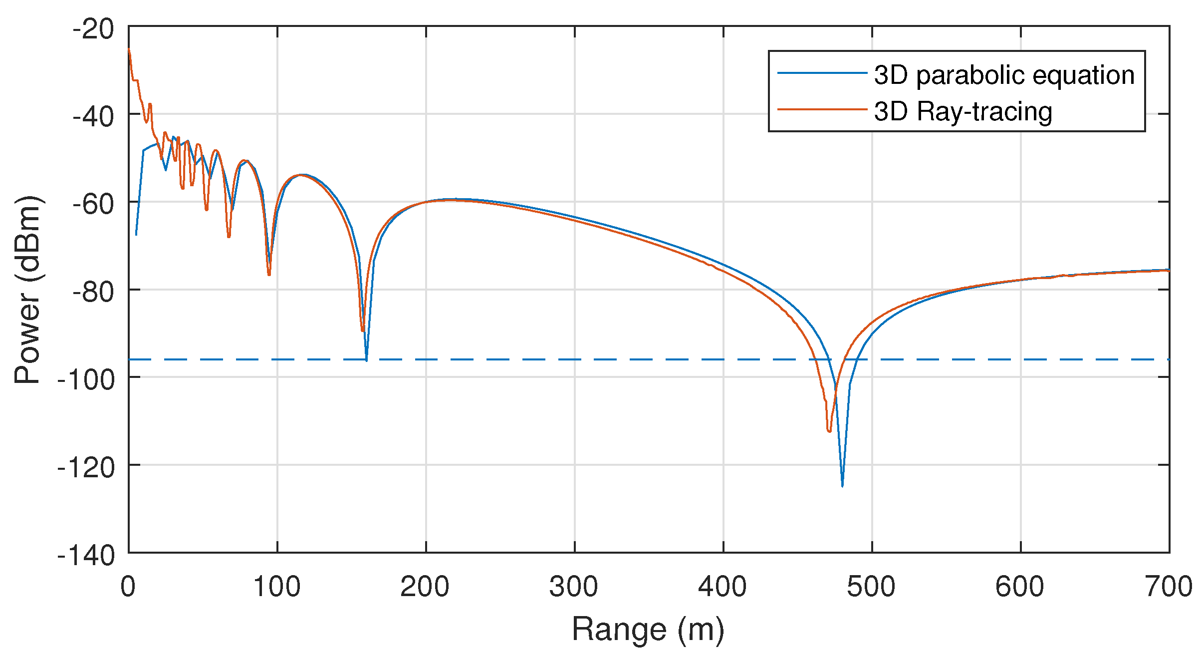
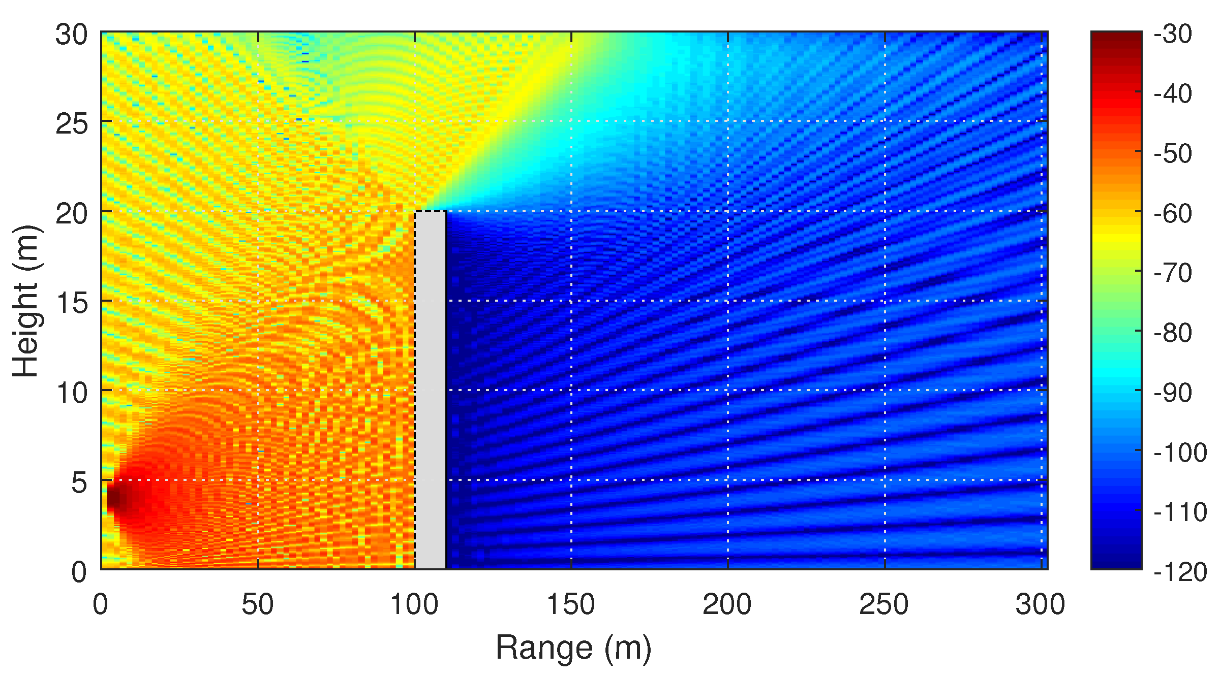
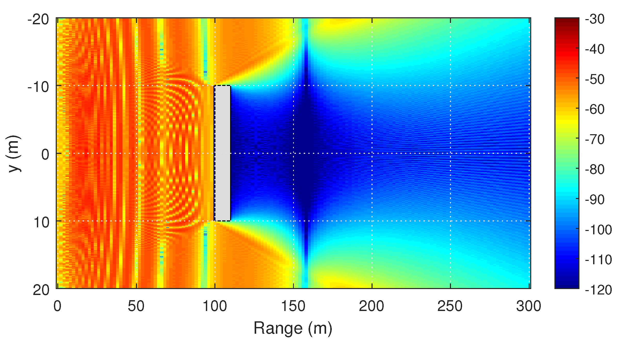
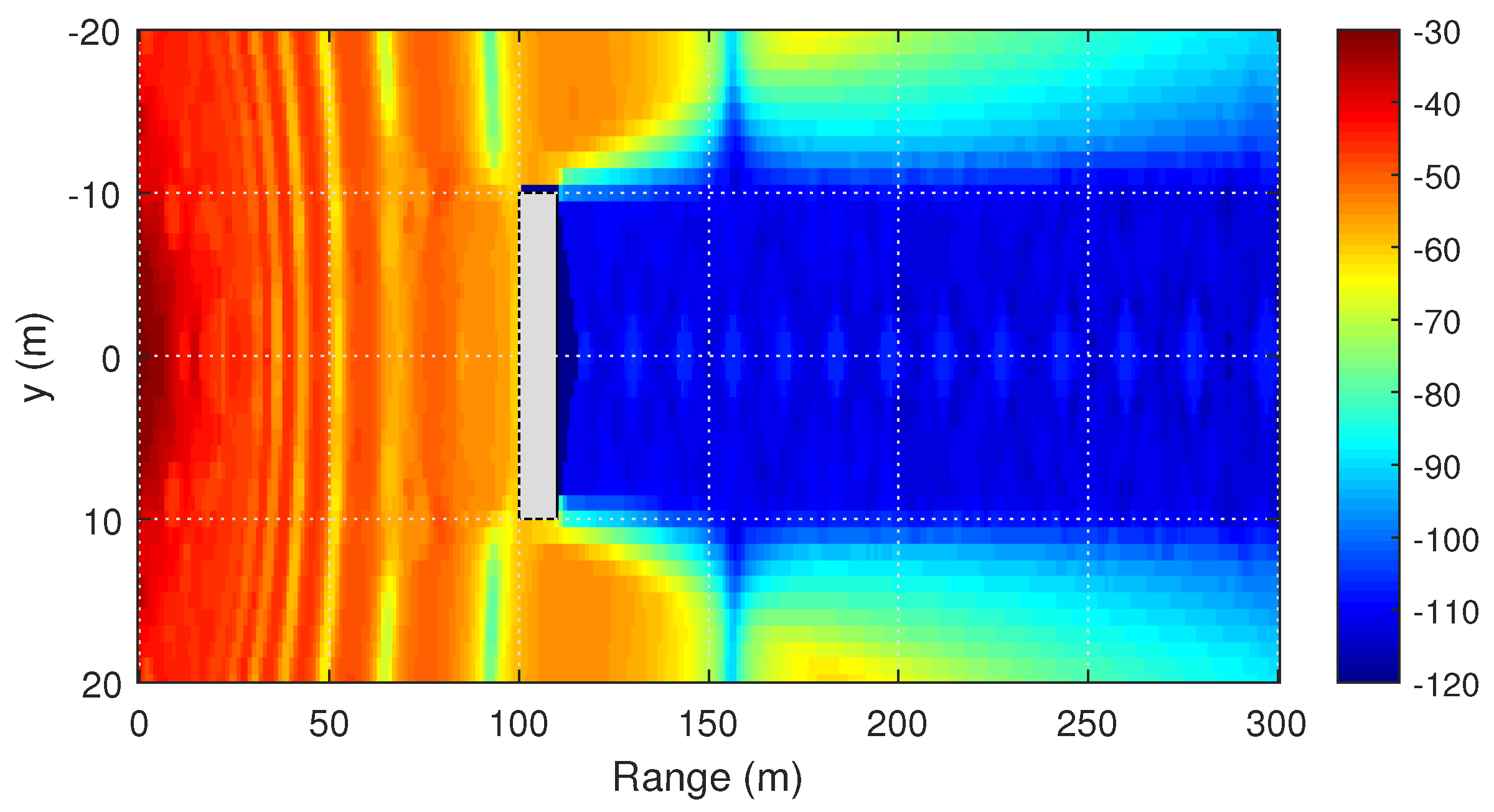
4.2. Diffraction on a Single Building

The following example shows wave propagation in the presence of a single building. The building is modeled through the PEC cuboid with shape 10 m × 20 m × 20 m. Figure 2 demonstrates the two-dimensional distribution against range and height, obtained by the two-way PE method.

The backscattering from the obstacle, modeled by the bidirectional PE, is clearly visible. Figure 3 and Figure 4 demonstrate the two-dimensional distribution of the signal level at the height of 1.5 m, obtained by the PE and RT methods, respectively.

In general, both methods produce similar results.

One can clearly see from Figure 5, that the field behind the building is significantly lower than the threshold −96 dBm. The loss behind the obstacle is about 50 dBm. It can be concluded that it is almost impossible for the radio waves to overcome buildings from above within the considered frequency and power of the transmitter. Thus, if the height of buildings is not known during modeling, it can be considered infinite without much loss of accuracy.

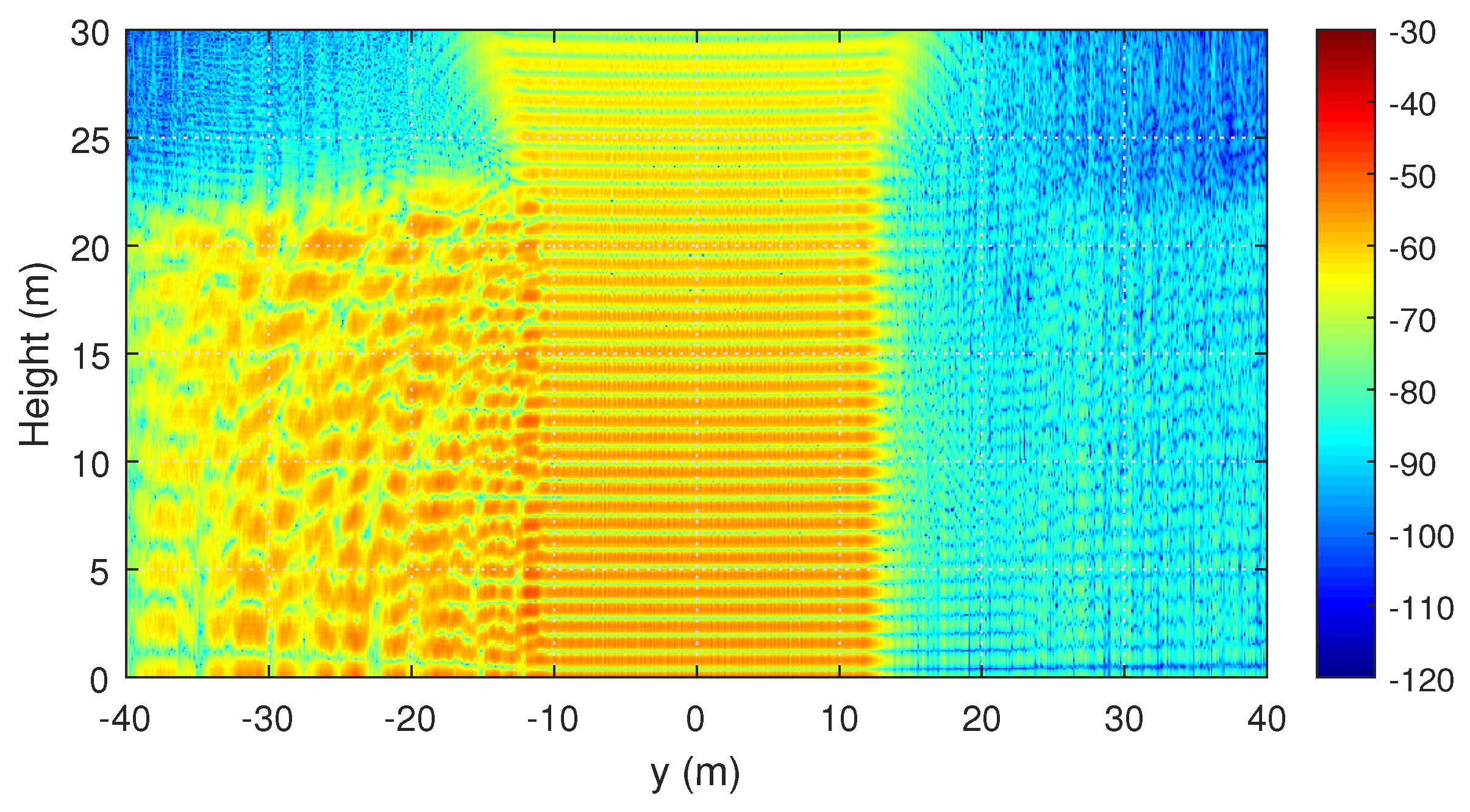
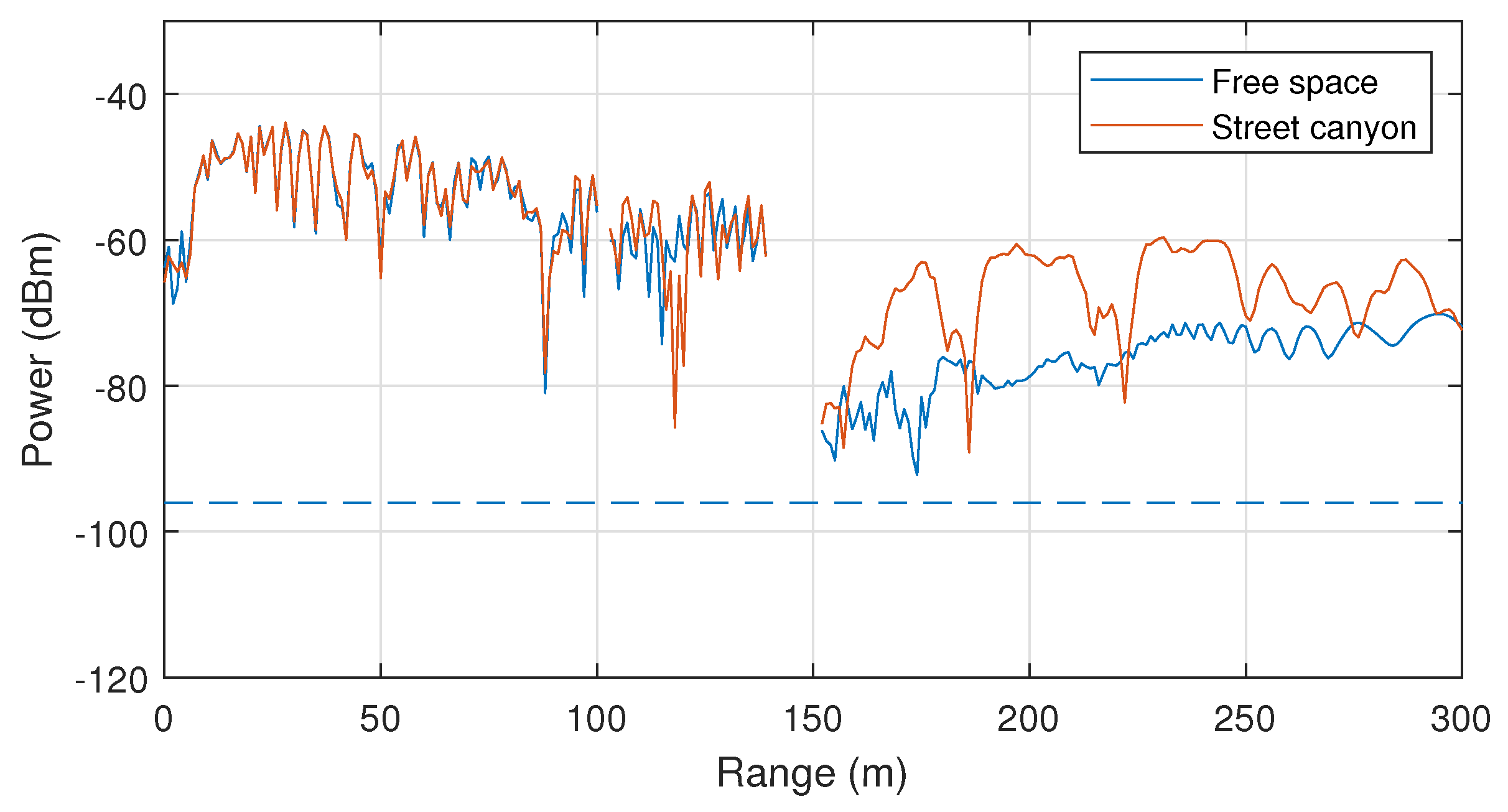
4.3. Propagation in a Street Canyon

The following example shows the propagation of 5900 MHz waves in a street canyon waveguide. The width of the canyon is 20 m and the buildings are 20 m high. Again, all surfaces are PEC. The projections of the field on the planes $xz$ and $xy$ are depicted in Figure 6 and Figure 7, respectively.

Figure 8 shows a comparison of the signal strength in free space (as in first example) and in a street canyon. It is clearly seen that the interference pattern caused by the ground surface is supplemented by the interference caused by reflection from buildings. This leads to even more significant fluctuations in the signal level depending on the distance. Interference minima can lead signal to fade at certain distances from the source.

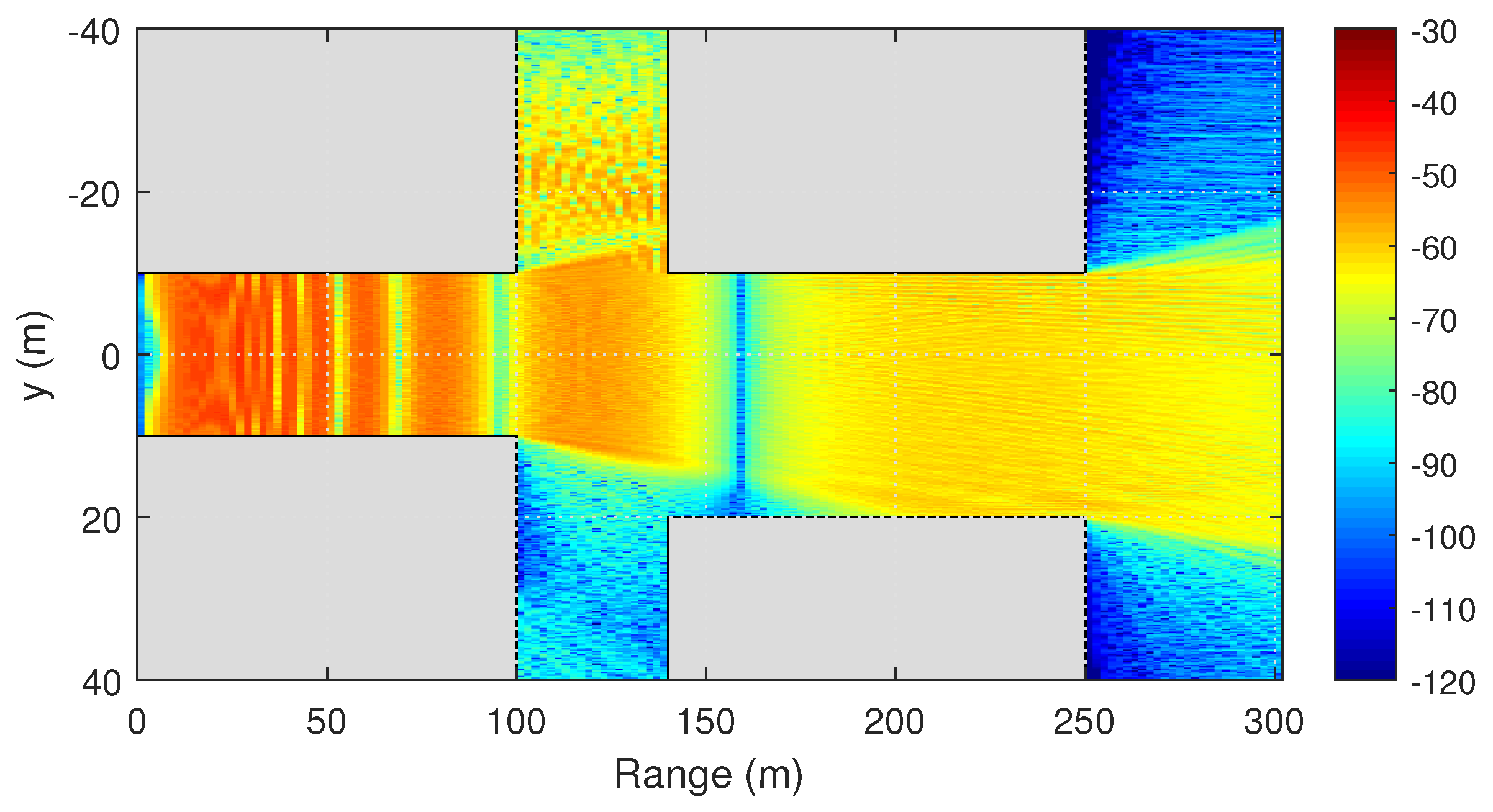
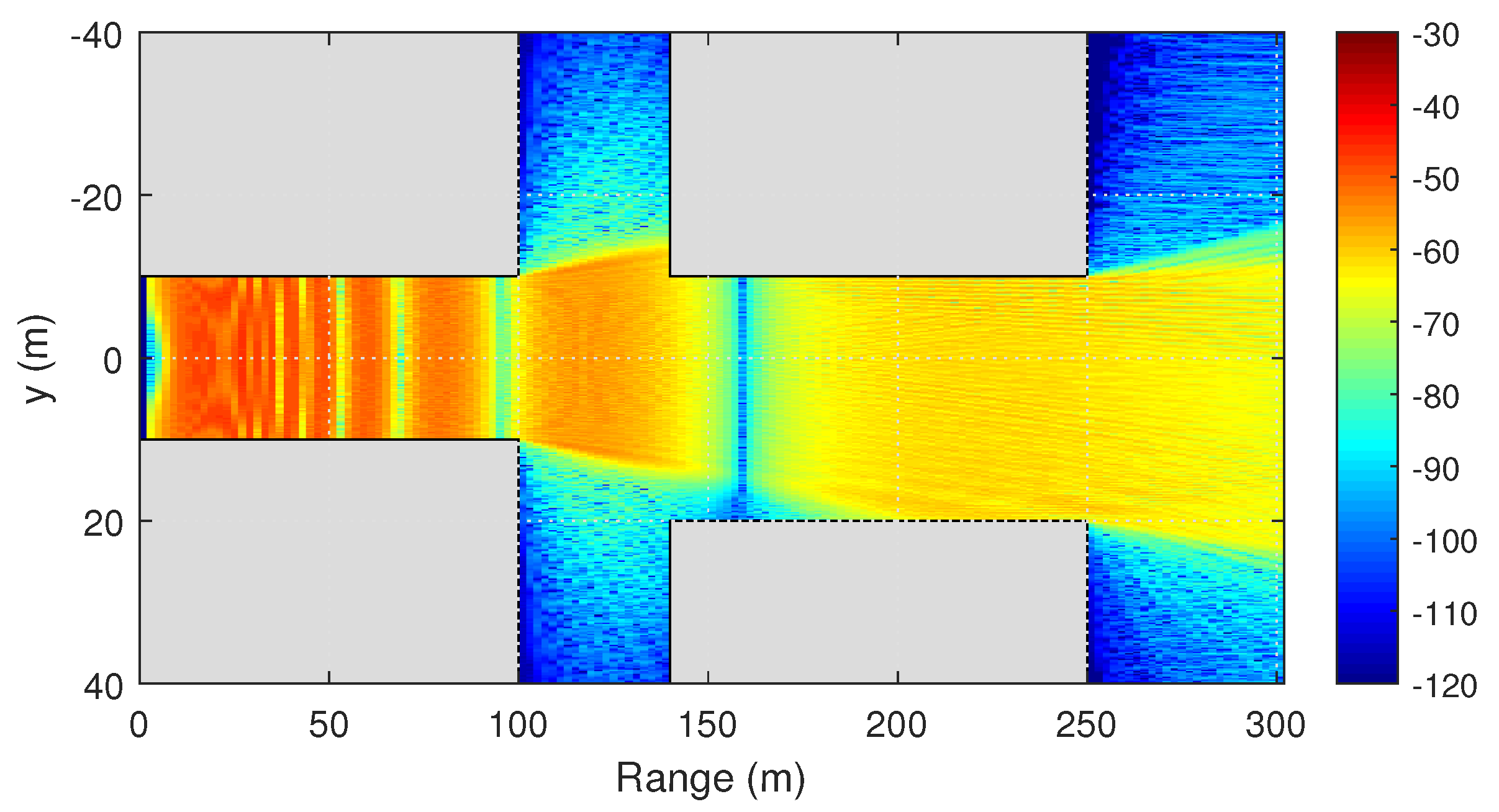
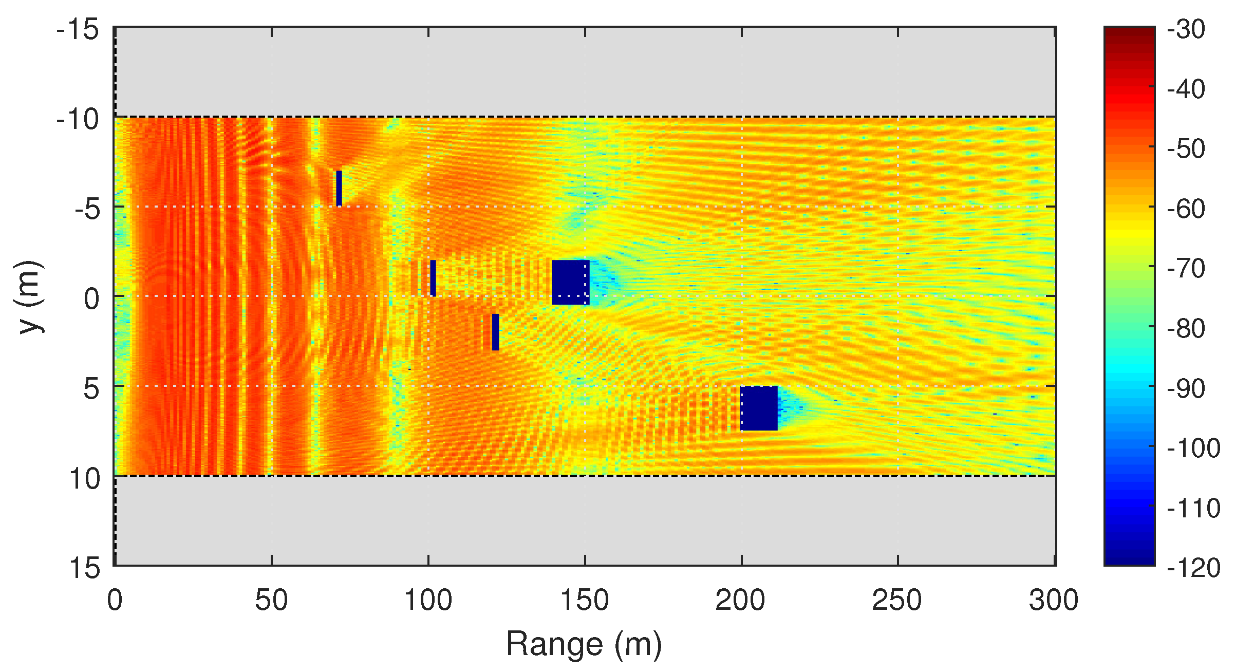
4.4. Diffraction on a Crossroad

Next, we consider the propagation of radio waves through the crossroad. The crossroad is located at a distance of 100 m from the source. Figure 9 and Figure 10 demonstrate the two-dimensional distribution of the field at the height of 1.5 m, calculated by two-way and one-way PE method, respectively.

Due to the diffraction, some of the energy gets to the next street. Further, this energy is propagated by reflection from buildings. This is clearly seen when comparing the results obtained by the one-way and two-way PE methods. Due to diffraction and reflection, a sufficiently strong signal level can be achieved even outside the line of sight. However, this effect depends significantly on the geometry of the propagation medium and obstacles location. For example, one can see from Figure 11, that the waves propagate much better to the left side of the road than to the right. This is due to the mutual location of the buildings in the considered example.

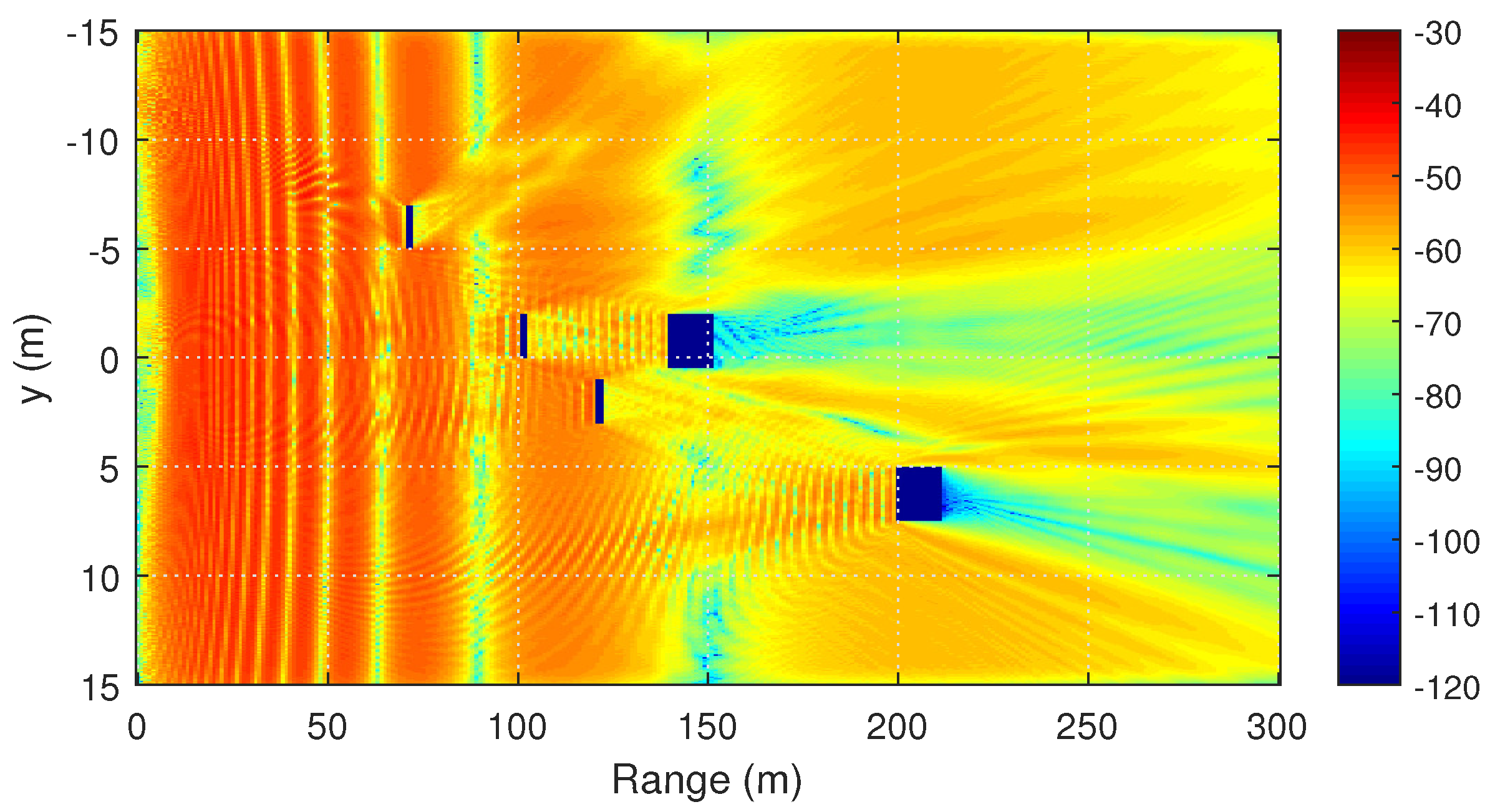
4.5. Impact of Car Traffic

In the final example, we will analyze the influence of automobiles and buses on the propagation of radio waves. Passenger cars and busses are modeled by a PEC cuboid with shapes 4 m × 2 m × 1.5 m and 12 m × 2.5 m × 3 m, respectively. Figure 12 shows scattering of radio waves on three cars and two buses, with no other obstacles.

In Figure 13 similarly positioned vehicles are placed in a 20 m wide street canyon. It can be seen that passenger cars do not significantly affect the electromagnetic field distribution.

At the same time, buses contribute to field attenuation of 20 dBm at the height of 1.5 m directly behind them. One can see from Figure 14, that reflections from buildings in a street canyon stimulate to significantly compensate for the shadow zone behind a massive road obstacles. In free space without buildings, the field level behind the obstacle remains 10–20 dBm lower.

5. Conclusions

Line-of-sight propagation is possible at distances exceeding 700 m from the source within the specifications of the problem under consideration. Signal reception is also possible in non-line-of-sight, but it significantly depends on the relative location of buildings in the propagation area. Passenger cars do not significantly affect the signal strength. Trucks and buses can contribute to 10–20 dBm attenuation. At the same time, the impact of traffic is more noticeable in free space without massive obstacles than in the street canyon waveguide. The height of buildings does not have a significant impact on the propagation, since waves at the considered frequency of 5900 MHz with a typical emitter power of 27 dBm are practically not able to overcome buildings from above if its height exceeds four to five floors.

The three-dimensional two-way PE method can be effectively applied to the radio wave propagation problem in urban development. Despite the relatively small wavelength (0.05 m), the three-dimensional two-way PE method made it easy to calculate the field at a distance of up to 700 m from the source. In all the considered examples, the calculation time of the PE method did not exceed 10 min. Interference, diffraction, scattering, and reflection can be effectively modeled within the proposed approach. The comparison with the RT method also proves the adequacy of the proposed model. The proposed method can be used for direct field calculation in complex urban conditions as well as for calibration and verification of simple empirical models.

Of course, the proposed approach in its present formulation is far from competing with specially elaborated empirical and RT-based models in real-world scenarios. In this paper, we did not consider complex impedance boundary conditions and depolarization effects. However the PE method, in principle, can handle them after a certain modification, which should be carried out in the future. Vegetation can be further modeled by the spatial variations in the refractive index. Time variance may be also accounted for within the proposed approach [48]. In this paper, we used the implementation of SSF on the CPU. However, given the good parallelizability of multidimensional discrete Fourier transforms, it is possible to achieve a significant increase in performance by using the GPU in the future. The indisputable advantage of the proposed method is its strong theoretical basis. There are reasons to believe that after several modifications of the proposed method, it can be effective in a wide class of real-world applications.

Matlab implementation of the proposed approach, developed by the authors, is freely available in Lytaev [47].

References

1. Liang, L.; Peng, H.; Li, G.Y.; Shen, X. Vehicular communications: A physical layer perspective. IEEE Trans. Veh. Technol. 2017, 66, 10647–10659. [Google Scholar] [CrossRef]
2. Vladyko, A.; Khakimov, A.; Muthanna, A.; Ateya, A.A.; Koucheryavy, A. Distributed edge computing to assist ultra-low-latency VANET applications. Future Internet 2019, 11, 128. [Google Scholar] [CrossRef] [Green Version]
3. Elagin, V.; Spirkina, A.; Buinevich, M.; Vladyko, A. Technological Aspects of Blockchain Application for Vehicle-to-Network. Information 2020, 11, 465. [Google Scholar] [CrossRef]
4. Viriyasitavat, W.; Boban, M.; Tsai, H.M.; Vasilakos, A. Vehicular communications: Survey and challenges of channel and propagation models. IEEE Veh. Technol. Mag. 2015, 10, 55–66. [Google Scholar] [CrossRef] [Green Version]
5. Lytaev, M.S.; Vladyko, A.G. Comparative Analysis of Parabolic Equation Method and Longley–Rice Propagation Model. In Proceedings of the IEEE 2019 11th International Congress on Ultra Modern Telecommunications and Control Systems and Workshops (ICUMT), Dublin, Ireland, 28–30 October 2019; pp. 1–5. [Google Scholar]
6. Urquiza-Aguiar, L.; Tripp-Barba, C.; Estrada-Jiménez, J.; Igartua, M.A. On the impact of building attenuation models in vanet simulations of urban scenarios. Electronics 2015, 4, 37–58. [Google Scholar] [CrossRef] [Green Version]
7. Nilsson, M.G.; Gustafson, C.; Abbas, T.; Tufvesson, F. A path loss and shadowing model for multilink vehicle-to-vehicle channels in urban intersections. Sensors 2018, 18, 4433. [Google Scholar] [CrossRef] [PubMed] [Green Version]
8. Yang, M.; Ai, B.; He, R.; Wang, G.; Chen, L.; Li, X.; Huang, C.; Ma, Z.; Zhong, Z.; Wang, J.; et al. Measurements and Cluster-Based Modeling of Vehicle-to-Vehicle Channels With Large Vehicle Obstructions. IEEE Trans. Wirel. Commun. 2020, 19, 5860–5874. [Google Scholar] [CrossRef]
9. Li, W.; Hu, X.; Gao, J.; Zhao, L.; Jiang, T. Measurements and Analysis of Propagation Channels in Vehicle-to-Infrastructure Scenarios. IEEE Trans. Veh. Technol. 2020, 69, 3550–3561. [Google Scholar] [CrossRef]
10. ITU-R. Recommendation P.1411. Propagation Data and Prediction Methods for the Planning of Short-Range Outdoor Radiocommunication Systems and Radio Local Area Networks in the Frequency Range 300 MHz to 100 GHz. 2019. Available online: https://www.itu.int/dms_pubrec/itu-r/rec/p/R-REC-P.1411-10-201908-I!!PDF-E.pdf (accessed on 26 November 2020).
11. Rappaport, T.S.; Xing, Y.; MacCartney, G.R.; Molisch, A.F.; Mellios, E.; Zhang, J. Overview of Millimeter Wave Communications for Fifth-Generation (5G) Wireless Networks—With a Focus on Propagation Models. IEEE Trans. Antennas Propag. 2017, 65, 6213–6230. [Google Scholar] [CrossRef]
12. Yun, Z.; Iskander, M.F. Ray tracing for radio propagation modeling: Principles and applications. IEEE Access 2015, 3, 1089–1100. [Google Scholar] [CrossRef]
13. Valle, L.; Pérez, J.R.; Torres, R.P. Characterisation of Indoor Massive MIMO Channels Using Ray-Tracing: A Case Study in the 3.2–4.0 GHz 5G Band. Electronics 2020, 9, 1250. [Google Scholar] [CrossRef]
14. Green, D.; Yun, Z.; Iskander, M.F. Path loss characteristics in urban environments using ray-tracing methods. IEEE Antennas Wirel. Propag. Lett. 2017, 16, 3063–3066. [Google Scholar] [CrossRef]
15. Saito, K.; Fan, Q.; Keerativoranan, N.; Takada, J.i. Site-Specific Propagation Loss Prediction in 4.9 GHz Band Outdoor-to-Indoor Scenario. Electronics 2019, 8, 1398. [Google Scholar] [CrossRef] [Green Version]
16. Granda, F.; Azpilicueta, L.; Vargas-Rosales, C.; Lopez-Iturri, P.; Aguirre, E.; Astrain, J.J.; Villandangos, J.; Falcone, F. Spatial characterization of radio propagation channel in urban vehicle-to-infrastructure environments to support WSNS deployment. Sensors 2017, 17, 1313. [Google Scholar] [CrossRef] [Green Version]
17. Granda, F.; Azpilicueta, L.; Vargas-Rosales, C.; Celaya-Echarri, M.; Lopez-Iturri, P.; Aguirre, E.; Astrain, J.J.; Medrano, P.; Villandangos, J.; Falcone, F. Deterministic propagation modeling for intelligent vehicle communication in smart cities. Sensors 2018, 18, 2133. [Google Scholar] [CrossRef] [Green Version]
18. Granda, F.; Azpilicueta, L.; Celaya-Echarri, M.; Lopez-Iturri, P.; Vargas-Rosales, C.; Falcone, F. Spatial V2X Traffic Density Channel Characterization for Urban Environments. IEEE Trans. Intell. Transp. Syst. 2020. early access. [Google Scholar] [CrossRef]
19. MacKie-Mason, B.; Shao, Y.; Greenwood, A.; Peng, Z. Supercomputing-enabled first-principles analysis of radio wave propagation in urban environments. IEEE Trans. Antennas Propag. 2018, 66, 6606–6617. [Google Scholar] [CrossRef]
20. Levy, M.F. Parabolic Equation Methods for Electromagnetic Wave Propagation; The Institution of Electrical Engineers: London, UK, 2000. [Google Scholar]
21. Lytaev, M.S. Numerov-Pade scheme for the one-way Helmholtz equation in tropospheric radio-wave propagation. IEEE Antennas Wirel. Propag. Lett. 2020. early access. [Google Scholar] [CrossRef]
22. Lytaev, M.S.; Vladyko, A.G. Split-step Pade Approximations of the Helmholtz Equation for Radio Coverage Prediction over Irregular Terrain. In Proceedings of the IEEE 2018 Advances in Wireless and Optical Communications (RTUWO), Riga, Latvia, 15–16 November 2018; pp. 179–184. [Google Scholar]
23. Janaswamy, R. Path loss predictions in the presence of buildings on flat terrain: A 3-D vector parabolic equation approach. IEEE Trans. Antennas Propag. 2003, 51, 1716–1728. [Google Scholar] [CrossRef]
24. Zaporozhets, A. Application of vector parabolic equation method to urban radiowave propagation problems. IEE Proc. Microw. Antennas Propag. 1999, 146, 253–256. [Google Scholar] [CrossRef]
25. He, Z.; Zeng, H.; Chen, R. Two-way propagation modeling of expressway with vehicles by using the 3-D ADI-PE method. IEEE Trans. Antennas Propag. 2018, 66, 2156–2160. [Google Scholar] [CrossRef]
26. Li, Y.S.; Bian, Y.Q.; He, Z.; Chen, R.S. EM Pulse Propagation Modeling for Tunnels by Three-Dimensional ADI-TDPE Method. IEEE Access 2020, 8, 85027–85037. [Google Scholar] [CrossRef]
27. ITU-R. Recommendation ITU-R P.2040-1: Effects of Building Materials and Structures on Radiowave Propagation above about 100 MHz. 2015. Available online: https://www.itu.int/dms_pubrec/itu-r/rec/p/R-REC-P.2040-1-201507-I!!PDF-E.pdf (accessed on 26 November 2020).
28. Fock, V. Electromagnetic Diffraction and Propagation Problems; Pergamon Press: Oxford, UK, 1965. [Google Scholar]
29. Lytaev, M.S. Automated Selection of the Computational Parameters for the Higher-Order Parabolic Equation Numerical Methods. Lect. Notes Comput. Sci. 2020, 12249, 296–311. [Google Scholar]
30. Mikhailov, M.; Komarov, A. Extension of the parabolic equation method in the time domain. In Proceedings of the IEEE 2018 Progress in Electromagnetics Research Symposium (PIERS-Toyama), Toyama, Japan, 1–4 August 2018; pp. 357–361. [Google Scholar]
31. Born, M.; Wolf, E. Principles of Optics; Pergamon Press: Oxford, UK, 1980. [Google Scholar]
32. Kuttler, J.R.; Dockery, G.D. Theoretical description of the parabolic approximation/Fourier split-step method of representing electromagnetic propagation in the troposphere. Radio Sci. 1991, 26, 381–393. [Google Scholar] [CrossRef]
33. Ahdab, Z.E.; Akleman, F. Radiowave Propagation Analysis with a Bidirectional 3-D Vector Parabolic Equation Method. IEEE Trans. Antennas Propag. 2017, 65, 1958–1966. [Google Scholar] [CrossRef]
34. He, Z.; Chen, R.S. Frequency-domain and time-domain solvers of parabolic equation for rotationally symmetric geometries. Comput. Phys. Commun. 2017, 220, 181–187. [Google Scholar] [CrossRef]
35. Lytaev, M.S.; Vladyko, A.G. On Application of Parabolic Equation Method to Propagation Modeling in Millimeter-Wave Bands. In Proceedings of the IEEE 10th International Congress on Ultra Modern Telecommunications and Control Systems and Workshops (ICUMT), Moscow, Russia, 5–9 November 2018; pp. 332–337. [Google Scholar]
36. Apaydin, G.; Sevgi, L. The Split-Step-Fourier and Finite-Element-Based Parabolic-Equation Propagation- Prediction Tools: Canonical Tests, Systematic Comparisons, and Calibration. IEEE Trans. Antennas Propag. 2010, 52, 66–79. [Google Scholar] [CrossRef]
37. Taylor, M. Pseudodifferential Operators and Nonlinear PDE; Springer Science & Business Media: New York, NY, USA, 2012; Volume 100. [Google Scholar]
38. Bailey, D.H.; Swarztrauber, P.N. A fast method for the numerical evaluation of continuous Fourier and Laplace transforms. SIAM J. Sci. Comput. 1994, 15, 1105–1110. [Google Scholar] [CrossRef] [Green Version]
39. Davidson, D.B. Computational Electromagnetics for RF and Microwave Engineering; Cambridge University Press: New York, NY, USA, 2010. [Google Scholar]
40. Collins, M.D.; Evans, R.B. A two-way parabolic equation for acoustic backscattering in the ocean. J. Acoust. Soc. Am. 1992, 91, 1357–1368. [Google Scholar] [CrossRef]
41. Mills, M.J.; Collins, M.D.; Lingevitch, J.F. Two-way parabolic equation techniques for diffraction and scattering problems. Wave Motion 2000, 31, 173–180. [Google Scholar] [CrossRef]
42. Oraizi, H.; Hosseinzadeh, S. Radio-wave-propagation modeling in the presence of multiple knife edges by the bidirectional parabolic-equation method. IEEE Trans. Veh. Technol. 2007, 56, 1033–1040. [Google Scholar] [CrossRef]
43. Apaydin, G.; Ozgun, O.; Kuzuoglu, M.; Sevgi, L. A novel two-way finite-element parabolic equation groundwave propagation tool: Tests with canonical structures and calibration. IEEE Trans. Geosci. Remote Sens. 2011, 49, 2887–2899. [Google Scholar] [CrossRef]
44. Ozgun, O. Recursive two-way parabolic equation approach for modeling terrain effects in tropospheric propagation. IEEE Trans. Antennas Propag. 2009, 57, 2706–2714. [Google Scholar] [CrossRef]
45. Ozgun, O.; Apaydin, G.; Kuzuoglu, M.; Sevgi, L. PETOOL: MATLAB-based one-way and two-way split-step parabolic equation tool for radiowave propagation over variable terrain. Comput. Phys. Commun. 2011, 182, 2638–2654. [Google Scholar] [CrossRef]
46. Vavilov, S.A.; Lytaev, M.S. Modeling equation for multiple knife-edge diffraction. IEEE Trans. Antennas Propag. 2020, 68, 3869–3877. [Google Scholar] [CrossRef]
47. Lytaev, M.S. 3D 2-Way SSF Matlab Code. 2020. Available online: https://github.com/mikelytaev/3d-ssf (accessed on 26 November 2020).
48. Zhang, D.; Liao, C.; Feng, J.; Deng, X. Pulse-compression signal propagation and parameter estimation in the troposphere with parabolic equation. IEEE Access 2019, 7, 99917–99927. [Google Scholar] [CrossRef]
Figure 1. Propagation without obstacles. Distribution of the signal level at the height of 1.5 above the ground.
Electronics 09 02011 g001
Figure 2. Diffraction on a cuboid. Two-dimensional distribution of the signal level (dBm) calculated by the two-way PE method.
Electronics 09 02011 g002
Figure 3. Diffraction on a cuboid. Two-dimensional distribution of the signal level (dBm) at the height of 1.5 m, calculated by the two-way PE method.
Electronics 09 02011 g003
Figure 4. Diffraction on a cuboid. Two-dimensional distribution of the signal level (dBm) at the height of 1.5 m, calculated by the RT method.
Electronics 09 02011 g004
Figure 5. Diffraction on a cuboid. Distribution of the signal level at the height of 1.5 above the ground.
Electronics 09 02011 g005
Figure 6. Propagation in a street canyon. Two-dimensional distribution of the signal level (dBm) along the x axis, calculated by the PE method.
Electronics 09 02011 g006
Figure 7. Propagation in a street canyon. Two-dimensional distribution of the signal level (dBm) at the height of 1.5 m, calculated by the two-way PE method.
Electronics 09 02011 g007
Figure 8. Propagation in a street canyon. Distribution of the signal level at the height of 1.5 above the ground.
Electronics 09 02011 g008
Figure 9. Propagation in a crossroad. Two-dimensional distribution of the signal level (dBm) at the height of 1.5 m, calculated by the two-way PE method.
Electronics 09 02011 g009
Figure 10. Propagation in a crossroad. Two-dimensional distribution of the signal level (dBm) at the height of 1.5 m, calculated by the one-way PE method.
Electronics 09 02011 g010
Figure 11. Propagation in a crossroad. Two-dimensional distribution of the signal level (dBm) at the distance of 125 m from the source along a perpendicular street, obtained by the two-way PE method.
Electronics 09 02011 g011
Figure 12. Scattering on vehicles. Two-dimensional distribution of the signal level (dBm) at the height of 1.5 m, calculated by the two-way PE method.
Electronics 09 02011 g012
Figure 13. Scattering on vehicles in a street canyon. Two-dimensional distribution of the signal level (dBm) at the height of 1.5 m, calculated by the two-way PE method.
Electronics 09 02011 g013
Figure 14. Scattering on vehicles. Distribution of the signal level at the height of 1.5 above the ground.
Electronics 09 02011 g014
Publisher’s Note: MDPI stays neutral with regard to jurisdictional claims in published maps and institutional affiliations.