Article

Group Teaching Optimization Algorithm Based MPPT Control of PV Systems under Partial Shading and Complex Partial Shading

by
Muhammad Hamza Zafar
1,
Thamraa Al-shahrani
2,*,
Noman Mujeeb Khan
1,
Adeel Feroz Mirza
3,
Majad Mansoor
3,
Muhammad Usman Qadir
4,
Muhammad Imran Khan
5 and
Rizwan Ali Naqvi
6,*
1
Department of Electrical, Capital University of Science and Technology, Islamabad 44000, Pakistan
2
Department of Physics, College of Science, Princess Nourah Bint Abdulrahman University, Riyadh 11671, Saudi Arabia
3
Department of Automation, University of Science and Technology of China, Hefei 230027, China
4
Department of Electrical, Islamabad Campus, University of Lahore, Islamabad 46000, Pakistan
5
Hefei National Lab for Physical Sciences at the Microscale and the Centers for Biomedical Engineering, University of Science and Technology of China, Hefei 230027, China
6
Department of Unmanned Vehicle Engineering, Sejong University, Seoul 05006, Korea
*
Authors to whom correspondence should be addressed.
Electronics 2020, 9(11), 1962; https://doi.org/10.3390/electronics9111962
Submission received: 22 October 2020 / Revised: 10 November 2020 / Accepted: 13 November 2020 / Published: 20 November 2020
(This article belongs to the Section Systems & Control Engineering)

Abstract

:
The most cost-effective electrical energy is produced by photovoltaic (PV) systems, and with the smallest carbon footprint, making it a sustainable renewable energy. They provide an excellent alternative to the existing fossil fuel-based energy systems, while providing 4% of global electricity demand. PV system efficiency is significantly reduced by the intrinsic non-linear model, maximum power point (MPP), and partial shading (PS) effects. These two problems cause major power loss. To devise the maximum power point tracking (MPPT) control of the PV system, a novel group teaching optimization algorithm (GTOA) based controller is presented, which effectively deals with the PS and complex partial shading (CPS) conditions. Four case studies were employed that included fast-changing irradiance, PS, and CPS to test the robustness of the proposed MPPT technique. The performance of the GTOA was compared with the latest bio-inspired techniques, i.e., dragon fly optimization (DFO), cuckoo search (CS), particle swarm optimization (PSO), particle swarm optimization gravitational search (PSOGS), and conventional perturb and observe (P&O). The GTOA tracked global MPP with the highest 99.9% efficiency, while maintaining the magnitude of the oscillation <0.5 W at global maxima (GM). Moreover, 13–35% faster tracking times, and 54% settling times were achieved, compared to existing techniques. Statistical analysis was carried out to validate the robustness and effectiveness of the GTOA. Comprehensive analytical and statistical analysis solidified the superior performance of the proposed GTOA based MPPT technique.

1. Introduction

Solar energy is utilized in commercial and standalone projects for electricity generation using concentrated solar and photovoltaic principles. Solar energy provides numerous merits, such as being abundant in nature, zero fuel cost, close to no carbon footprint, no mechanical maintenance, scalability, and ease of installation. In recent times, the output of photovoltaic (PV) energy has considerably increased; some estimations (explained by the International Renewable Energy Agency (IRENA)) identify that solar PV power capacity could reach 586 GW at the end of 2019 [1], with the major contributions from Japan (61.8 GW), Germany (49 GW), China (205 GW), India (34.8 GW), the USA (60.5 GW), and Italy (20.9 GW) [2]. As of 2020, the cost per watt is 1.654–1.6953 cents/KWh, which is the most cost-effective electrical energy [3,4].
A PV system is presented in Figure 1. The PV system is implemented with a DC–DC boost converter, which is used to control and regulate the output of the PV system. The maximum power point tracking (MPPT) controller controls the switching of the boost converter by the duty cycle. The purpose of forcing the PV system to operate on MPPT is to harvest the maximum available power at any instance of time. However, ever-altering operating conditions, temperature, irradiance, and sheltering by clouds, etc. cause nonlinearity and randomness in the behavior of the PV system, causing difficulties and challenges for MPPT controllers [5]. The MPPT controllers are classified into several categories which include classical and modern intelligent controllers. In classical controllers, perturb and observe (P&O), incremental conductance (IC), ripple correlation technique, short circuit current (SCC), and open-circuit voltage (OCV) are well-known techniques. The modern intelligent controllers are based upon the three main techniques namely fuzzy logic controllers (FLC) [6], neural networks (NN) [7,8], and swarm intelligence (SI) [8]. The most common benefits one achieves by using these intelligent controllers are high efficiency, robustness, and ability to tackle the MPPT problem with the least accurate mathematical modeling of the system, meanwhile, classical techniques pose major drawbacks, discussed later [9].
In the literature many MPPT techniques have been proposed, and depending upon the accuracy, techniques vary significantly by the type of control strategies. Voltage, current, and duty cycle are utilized, along with a mathematical model of PV cells, to devise fundamental techniques, and are utilized to predict optimized operating points on the P–V curve. In open circuit voltage (OCV), V O C is used similarly, and I S C is utilized to model MPPT control [10]. In this model mathematical approximations are utilized to predict the operating point, and no real-time monitoring of output power is involved, so the accuracy cannot be reliable. Moreover, the operating point is not reliable because the I–V and P–V curves show the dependence upon operating conditions, and hence efficiency is compromised [11].
The simplest and most famous classical MPPT technique is the P&O algorithm. In the perturb and observe (P&O) method, a predefined small change is introduced to perturb the system, consequently, the observed values are calculated and a power comparison yields the direction of change on the P–V curve. It is a simple and effective technique, and has been implemented in standalone and hybrid modes. However, like other techniques, it does also offer certain critical drawbacks, such as the oscillations caused by the differential increase in duty cycle. To minimize these oscillations, the step size has to be small, which consequently causes a dip in tracking time. Hence, there is a tradeoff between tracking time and efficiency in this technique. Incremental conductance (IC) is yet another technique which utilizes the change in instantaneous conductance with respect to current operating point to decide the direction of the operating point. In both P&O and IC, if the power (P) is improved, the direction of increment is retained and vice versa [12]. These techniques are easy to implement and are low cost. Under rapidly changing ambient conditions their draw backs become prominent and they fail to track actual MPP, due to their lack in properties, in terms of adaptively and robustness. Another technique known as the hill climbing (HC) mechanism utilizes direct control action. It suffers from similar drawbacks. Work done to improve the step size of the aforementioned techniques, improved the performance and efficiency but increased the complexity, and required accurate sensors. A comprehensive mathematical model integration with operating PV conditions is cumbersome, moreover, a partial shading scenario, and intrinsic oscillations could not be minimized significantly [13].
In an instance when PV system does not receive equal levels of irradiance, PS happens. The mismatch of produced current and voltage activates the PS effect. Isolated under shaded modules of arrays, bypass diodes in the antiparallel configuration are introduced. Initiation of bypass diodes produces multiple local maxima in I–V and P–V characteristic curves. It is observed that the number of peaks on a P–V curve is equal to the number of partially shaded modules connected in a series string of arrays. Local maxima (LM) and global maxima (GM) are two categories of maxima. There is only one GM, and the point of operation is called global maximum power point (GMPP). Classical techniques cannot differentiate among multiple maxima, hence considerable power is lost [14,15,16].
To counter the major issue of PS, many bio inspired techniques have been introduced recently. In the last decade a new class of bio-inspired algorithms have arisen. Meta-heuristics algorithms, which include particle swarm optimization (PSO) [17,18], artificial bee colony (ABC) [19], simulated annealing (SA) [20], cuckoo search (CS) [21,22], ant colony optimization (ACO) [23], moth fly optimization (MFO) [24], grey wolf optimization (GWO) [25], and pattern search (PS) [26] have recently proven to be effective for global optimization problems. There are many factors on which the performance of bio-inspired optimization techniques depend, namely population size, number of iterations, convergence speed, information sharing mechanism, computational time, and parametric tuning [27,28,29,30].
To share information regarding the best position, the PSO based MPPT technique uses the social interaction of swarm particles to share information. This information sharing is carried out using a weighted vector, which influences the position update of swarm particles, and helps the swarm particles to converge to the global solution. To break the LM trap, random numbers are embedded in velocity and position update equations. Random numbers produce unwanted oscillations and affect the settling time. The particle swarm optimization gravitational search (PSOGS) incorporates the effective exploration of PSO, with the accurate exploitation of GS, and improvises the working of PSO significantly. Although improvement in steady-state oscillations is observed, settling time is not significantly minimized. GS integration with PSO increases the number of parameters to be fine-tuned, the complexity of the technique, and the computational burden. ACO uses pheromones to share the information, which evaporate with time. Individually every ant is a member of a set representing a probable solution, so a cautious selection mechanism is required. Scout ants are also utilized to explore the search space [29]. In CSA random values are assigned using Levy flight, which causes unwanted fluctuations in output [20]. Lower population size makes these shortcomings meaningfully higher. A higher population number is utilized, which takes a toll on computation power and the time required to track GM. The main qualities required from bio-inspired techniques are quick convergence, least random oscillations, GM detection, robustness, and high power convergence. Although CSA, GHO, and PSOGS show reasonable tracking ability, the logical flow of these techniques involves randomness, and is more complex than the ordinary PSO algorithm, which makes their real-world implementation challenging [30].
Hybrid MPPT control takes advantage of robust conversion of classical techniques, and the SI techniques can be based upon the physical laws of nature, such as the swarming behavior of communal species. To overcome the drawbacks of the existing techniques by improving the performance over the iterative time, a new bio-inspired meta-heuristic algorithm group teaching optimization algorithm (GTOA) [31] was utilized to implement direct control of PV systems for the MPPT problem. Its ability to track GM was phenomenal. A comprehensive statistical and analytical study validated the superior performance of the proposed GTOA based MPPT for various weather conditions. A wide-ranging study was made to authenticate the effectiveness and robustness of the GTOA in this study. The major contribution of the proposed GTOA based MPPT techniques are
  • The introduction of a novel implementation of GTOA based MPPT technique for the partial shading problem of the PV system. The exploration and exploitation of search space are controlled by parameter “b” and “c” for maximizing the GM identification and quicker tracking of GM.
  • GTOA is effective in the optimization of uni-modal, multi-modal, and complex mathematical problems. The proposed GTOA has increased the overall tracking efficiency.
  • The best solution is attained in the mechanism and used to converge the population. Meanwhile, the rest of the swarm particles iteratively search the space, due to which performance is not compromised. A comprehensive analysis was done using extensive case studies, and specifically CPS was elaborated.

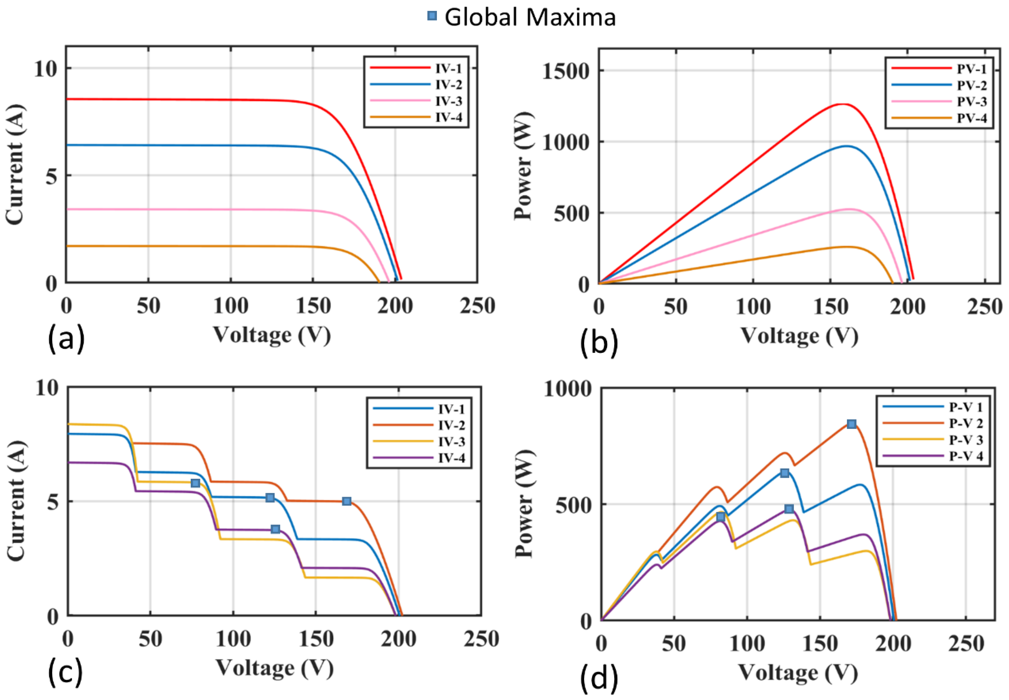
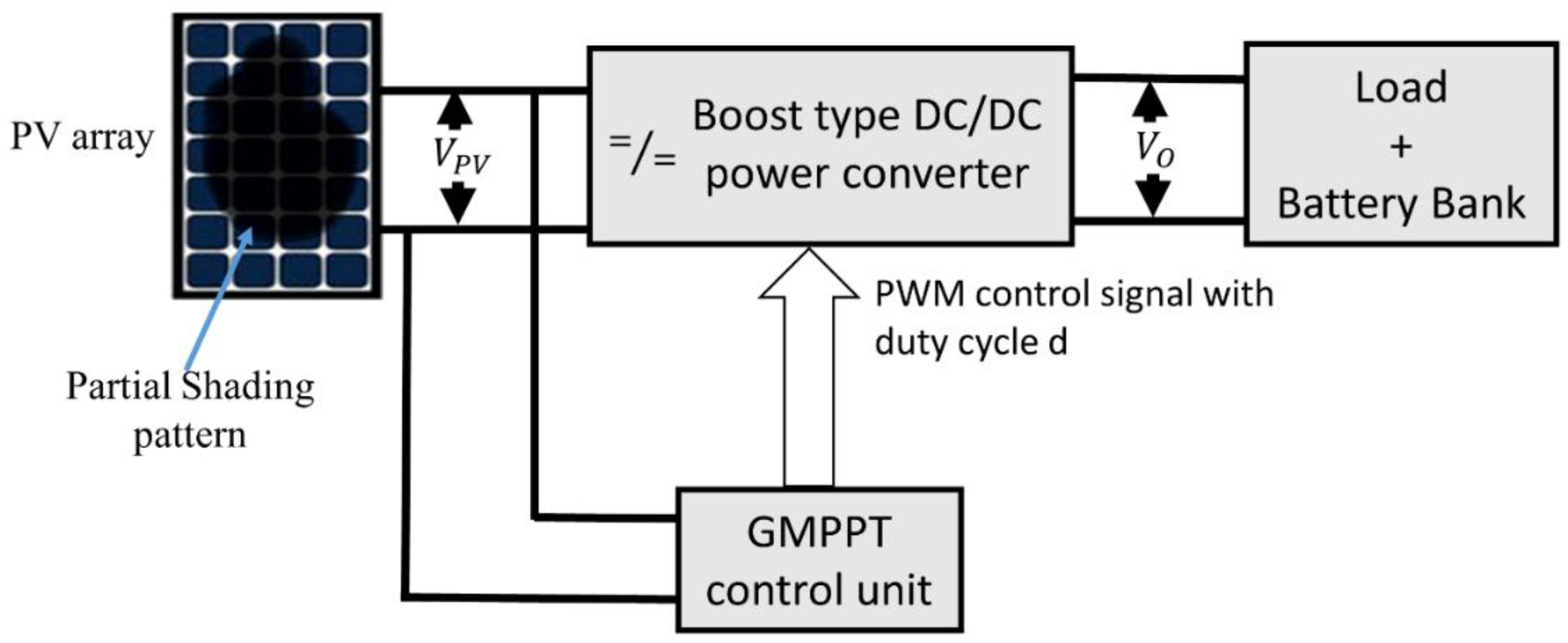
2. PV Cell Modeling and Behavior under Uniform Irradiance and PS Conditions

2.1. PV Model

To model the PV electrical characteristics of a solar cell, an equivalent single diode model is presented in Figure 2. The resistances added by parallel and series connections are integrated in the model.
I p v h is the current produced which is directly proportional to the incidence of light. The current through diode is I o and the current ( I ) flowing towards the output is shown in Equation (1).
I = I p v h I o
I = I p v h I s   ( exp ( V α V T ) 1 )
I = I p v h I s   ( exp ( V + I R s α V T ) 1 )
V T = N s K T q
The practical model of PV cell is modeled by adding intrinsic resistances, i.e., R s h is the series resistance, and R p h is the parallel resistance. The mathematical modeling is shown in Equation (3). A “Sunpreme SNPM-GX-315” solar panel was utilized in this study, and the electrical characteristics are shown in Table 1.

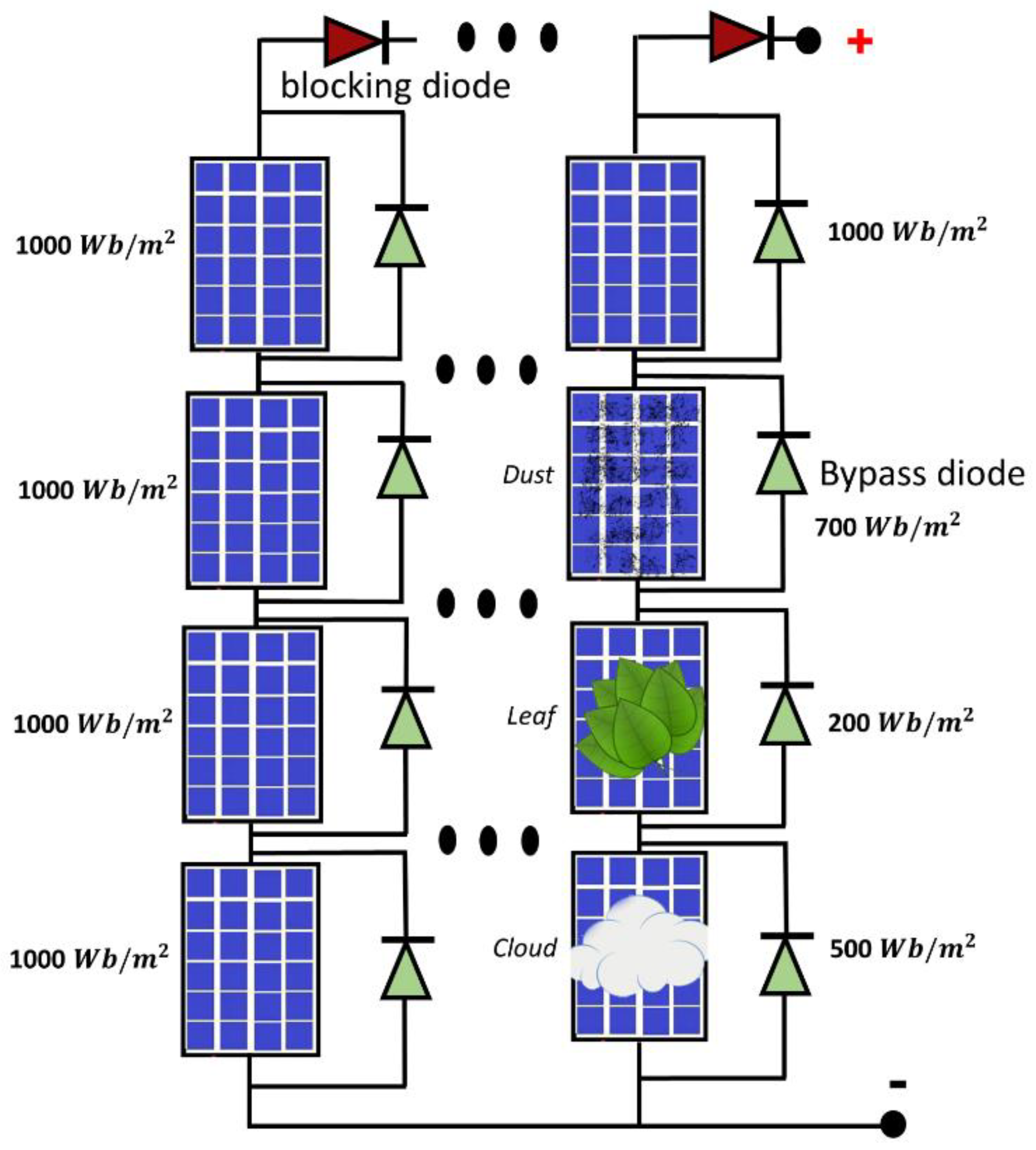
2.2. Partial Shading Condition

Under static irradiance, if all the PV panels are connected in series, the knee point of the I–V and P–V curve is the GMPP, as shown in Figure 3a,b, respectively.
When light of different irradiance falls on the series of connected modules, partial shading occurs. In the PS condition, the PV panels produce a non-uniform current, which causes hot spots and mismatching effects. The bypass diode appears as a viable solution to reduce these effects, which produce peaks with different magnitudes in I–V and P–V characteristic curves, as shown in Figure 3c,d. Figure 4 shows the PV panels under static and non-static irradiance, with bypass and blocking diodes. The number of peaks in I–V and P–V characteristic curves depends upon the number of panels receiving non-uniform irradiance. Due to PS, there is one GM and multiple LMs.

3. MPPT Using GTOA

A novel group teaching optimization algorithm was used for MPPT. The methodology of the proposed GTOA is explained in Section 3.

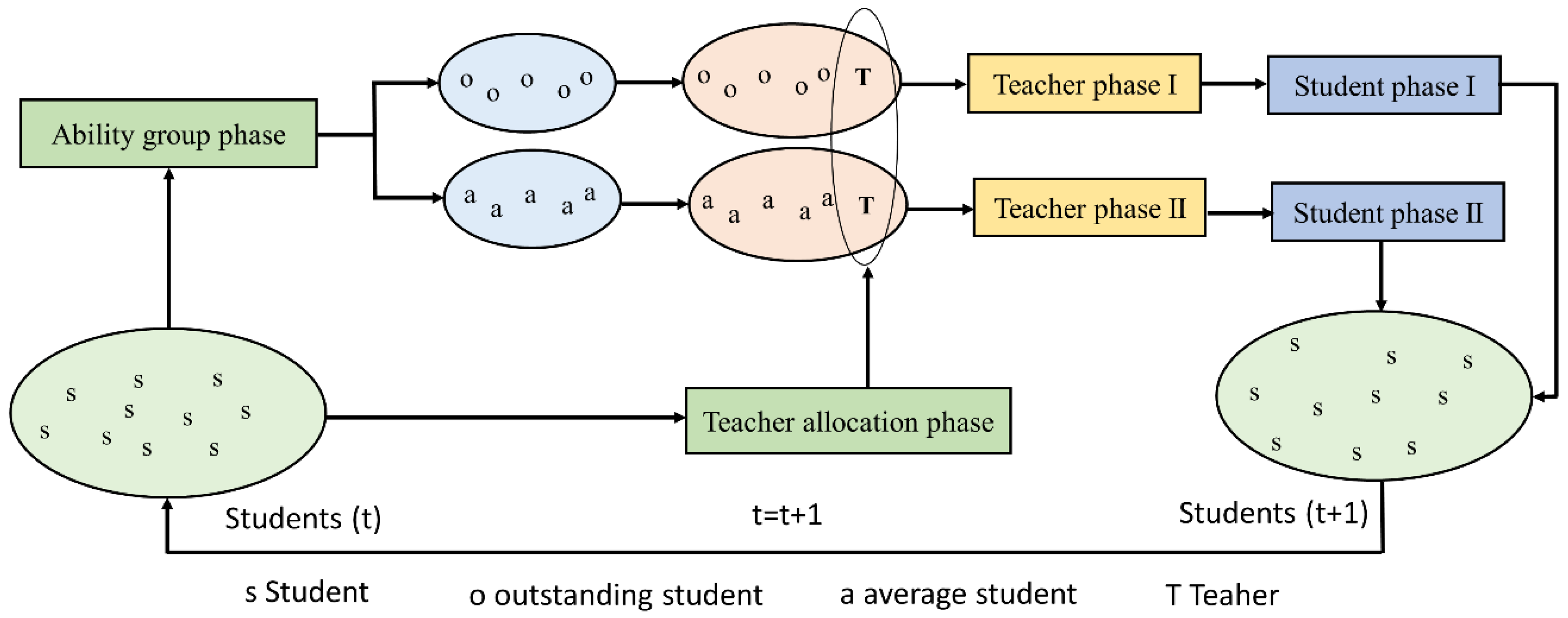
3.1. Framework of GTOA

A novel group teaching optimization algorithm was used for MPPT. By simulating a group teaching mechanism, the knowledge of the whole class (c) can be improved, which is the basic idea behind the proposed technique, i.e., GTOA. To implement the GTOA tor the optimization, a simple group of teaching model was presented based on the following rules.
  • The only difference between students is the capability to be acquiescent of knowledge. The greater challenge for the teacher to formulate the teaching plan depends upon the differences in ability to accept knowledge.
  • The quality of a good teacher is to pay additional attention to the students who have a poor capability to accept knowledge.
  • By self-learning, or by interacting with classmates, a student can improve his knowledge during the free time.
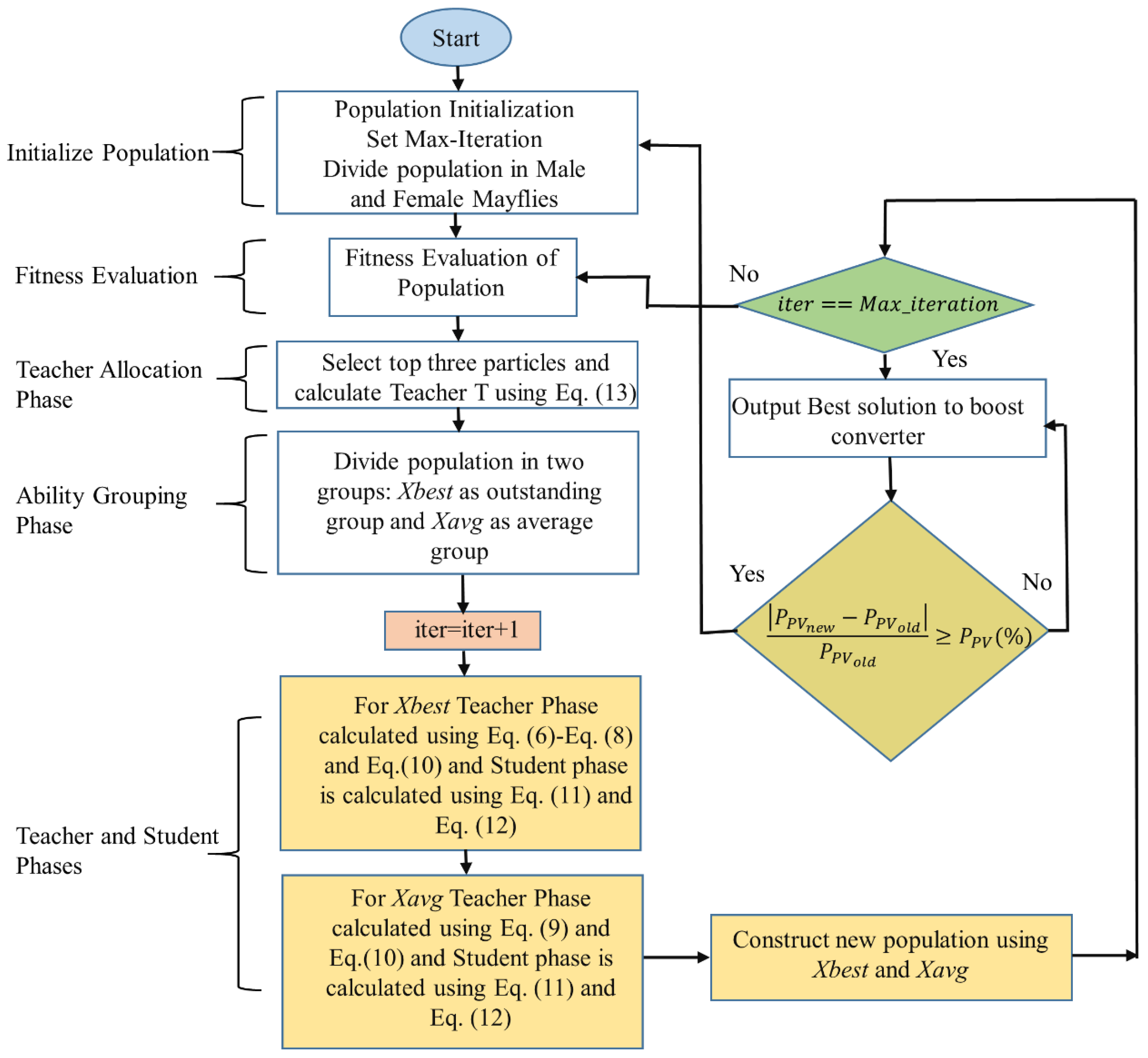
  • To improve the knowledge of students, a good teacher allocation method is helpful. Four phases are proposed in this model, which are represented in Figure 5.

3.1.1. Ability Grouping

To represent the knowledge of the whole class, a normal distribution function was used which is shown in Equation (5).
f ( x ) = 1 2 π δ e x p ( x μ ) 2
where x is value for which normal distribution function is required. μ is the mean and δ is the standard deviation. In group teaching optimization, all students are divided into two groups. An outstanding group is a group of students with a good ability to grasp knowledge, whereas the group with the poor capability to grasp knowledge is called the average group.

3.1.2. Teacher Phase

In this phase, students learn from the teacher, which is the second rule previously defined. In the GTOA the teacher makes separate plans for average and outstanding groups.
  • Teacher phase I:
The teacher focuses on improving the knowledge of the whole class due to the good ability of students to accept knowledge. Students belonging to an outstanding group can increase knowledge by Equation (6).
X t e a c h e r _ j t + 1 = X j t + a × ( T t F × ( B × M t + c × X j t ) )
M t = 1 N j = 1 N X j t
b + c = 1
where the number of students is represented by N , X j is the knowledge of each student, T is the teacher’s knowledge, M is the mean groups’ knowledge. Teacher factor is represented by F , X t e a c h e r _ j is the knowledge of student j learning from the teacher. Randomness is introduced by a , b , and c in the range (0,1).
  • Teacher phase II:
Due to weak knowledge accepting ability, based on the second rule, the teacher provides more attention to the average group. An average group of students can gain knowledge by Equation (9).
X t e a c h e r , j t + 1 = X j t +   2 × d × ( T t   X j t )
where d is randomness (0,1). Equation (10) addresses the problem where a student cannot get knowledge from the teacher phase.
X t e a c h e r , j t + 1 = { X t e a c h e r , j t , f ( X t e a c h e r , j t + 1 ) < f ( X j t ) X j t , f ( X t e a c h e r , j t + 1 ) f ( X j t )

3.1.3. Student Phase

In spare time students can gain knowledge by self-learning, or by interacting with fellow students, which can be represented mathematically as shown in Equation (11). The student phase links to the third rule by including student phases I and II.
X t e a c h e r , j t + 1 = { X t e a c h e r , j t + e × ( X t e a c h e r , j t + 1 X t e a c h e r , k t + 1 ) + g × ( X t e a c h e r , j t + 1 X j t ) , f ( X t e a c h e r , j t + 1 ) < f ( X t e a c h e r , k t + 1 ) X t e a c h e r , j t e × ( X t e a c h e r , j t + 1 X t e a c h e r , k t + 1 ) g × ( X t e a c h e r , j t + 1 X j t ) , f ( X t e a c h e r , j t + 1 ) f ( X t e a c h e r , k t + 1 )
where e and g are two randoms (0,1), X s t u d e n t , j   t + 1 is knowledge of the student j , and X t e a c h e r , j t + 1 is knowledge of the student j learning from the teacher. Students cannot gain knowledge in this phase. He or she can be addressed by Equation (12).
X j t + 1 = { X t e a c h e r , j t , f ( X t e a c h e r , j t + 1 ) < f ( X s t u d e n t , j t ) X s t u d e n t , j t , f ( X t e a c h e r , j t + 1 ) f ( X s t u d e n t , j t )

3.1.4. Teacher Allocation Phase

In order to improve the student’s knowledge, a good teacher allocation method is crucial, and which is defined by the fourth rule. Inspired by the hunting behavior of grey wolves, the top three best students are selected, as presented in Equation (13).
T = { X f i r s t t , f ( X f i r s t t ) f ( X f i r s t t + X s e c o n d t + X t h i r d t 3 ) X f i r s t t + X s e c o n d t + X t h i r d t 3 > f ( X f i r s t t + X s e c o n d t + X t h i r d t 3 )
where X f i r s t t , X s e c o n d t , and X t h i r d t are the top three students, respectively.

3.2. Working of GTOA as MPPT

GTOA works on the basis of group learning, which increases the efficiency and reduces the oscillations, due to the mean value of knowledge derived from the top three students. CPS conditions is explained in Figure 6. The tracking mechanism of GTOA’s particles in search space over the P–V curve is shown in Figure 7. Figure 7a shows the power tracked, Figure 7b is the P–V curve under PS conditions, and Figure 7c represents the transients in the reference voltage generated by GTOA. The Boost convert provides the necessary control and load interface given in Appendix A.
Partial shading occurs due to the difference in irradiance levels on PV modules connected in series. Due to bypass diodes, the modules connected in series create complex multiple peaks in the form of groups, called a cluster. In every cluster, the MPP is called the cluster head maxima (CHM). CPS conditions are shown in Figure 6. The left half-plane contains cluster 1, whose maxima is 1117 W . From left to right, the values of peaks in cluster 1 are 792.9 W , 958.3 W , 1028 W , 1117 W , and 1080 W . In the right half of the plane, cluster 2 contains GMPP whose value is 1136 W . The values of the local peaks in cluster 2 from left to right are 1136 W , 1128 W , 1035 W , and 828.4 W . The CHM in cluster 1 and GMPP has a difference of 19 W which is less than 2% of GMPP. Therefore, the re-initialization of the code will not occur.
Due to the complex partial shading, around 6% of power is lost due to the incorrect detection of GM. Due to incorrect initialization and mistuning of the parameter in bio-inspired techniques, the exploring populations gets stuck in the local maxima, and cause power loss. In GTOA, effective learning through grouping, proper re-initialization of code, and initialization of population give effective results in CPS.

Implementation of GTOA as MPPT

Implementation of GTOA as MPPT is presented in the flow chart shown in Figure 8. The step wise implementation is explained in Appendix B.

4. Results and Discussion

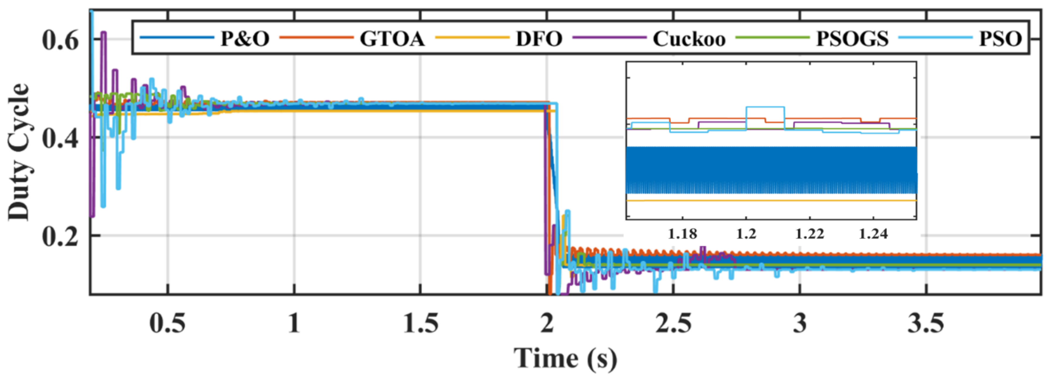
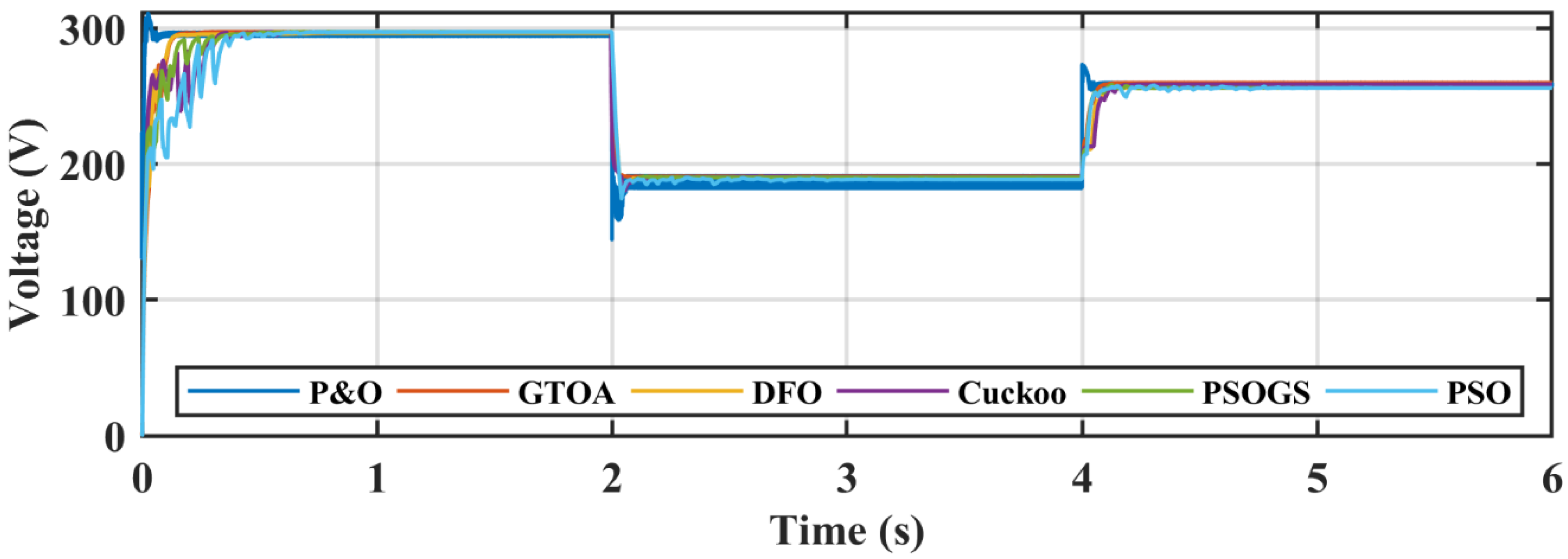
4.1. Case 1: Fast Varying Irradiance

Case 1 represents the fast varying irradiance pattern, to check the robustness of MPPT techniques in the tracking of mechanism power and re-tracking with changes in the weather conditions. After every 2 s, a change is produced in irradiance levels to reinitialize the MPPT technique to re-track the MPP. At 2 s irradiance level changed from 1000 W/m2 to 450 W/m2, and again at 4 s it changed to 750 W/m2, to test fast varying conditions. Irradiance levels are shown in Table 2.
Figure 9 and Figure 10 show the power tracked, and zoomed-in view of the power tracked. In the first interval at STC, the MP is 1264 W, and the power achieved by the GTOA, DFO, PSOGS, PSO, CS, and P&O, was 1263.5 W, 1262 W, 1260 W, 1263 W, 1263 W, and 1239 W, respectively.
Large oscillations can be observed in P&O around the GM, which cause power loss. In the first interval under STC, the efficiency achieved by GTOA, DFO, PSOGS, PSO, and CS was 99.96%, 99.84%, 99.68%, 99.92%, 99.92%, and 98.02%, respectively. PSO achieved higher efficiency compared to PSOGS, at the cost of higher fluctuations. To measure the performance of MPPT techniques, in terms of tracking power, the average power was taken.
In case 1 the average power was 921.3 W, and the average power tracked by GTO, DFO, PSOGS, PSO, CS, and P&O was 916.8 W, 905.8 W, 905 W, 903 W, 913 W, and 888 W, respectively. Re-initialization of particles under fast changing irradiance can be observed in Figure 11, in the duty cycle comparison at 2 s and 4 s. A zoomed-in duty cycle comparison can also be seen in Figure 12.
In order to measure the robustness of the MPPT techniques, tracking time and settling time are important tools. The time required by MPPT techniques to first track GM is called the tracking time, and the settling time is the time required by all SI particles to settle at GM. The tracking time of the GTOA, DFO, CS, PSO, PSOGS, and P&O was 0.135 s, 0.155 s, 0.41 s, 0.34 s, 0.31 s, and 0.1 s, and the settling time was 0.22 s, 0.24 s, 0.9 s, 0.62 s, 0.71 s, and 0.1 s, respectively. Voltage and current transient comparison is shown in Figure 13 and Figure 14.

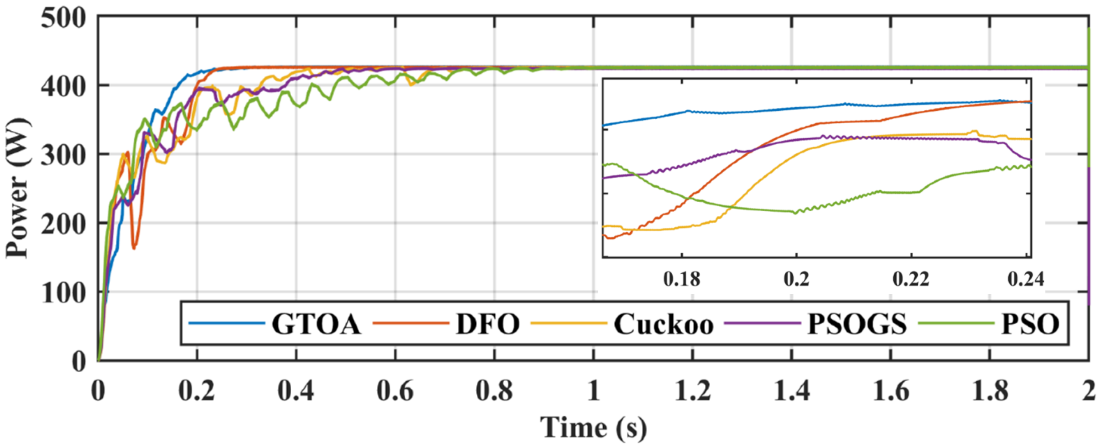
4.2. Case 2: Partial Shading

This case dealt with the PS condition, as mentioned in Figure 6, which contains multiple LMs and one GM. PSC was used to check the robustness of the MPPT technique. The irradiance pattern was 650 W/m2, 520 W/m2, 250 W/m2, and 400 W/m2. For case 2, MPP was at 427 W. Irradiance pattern is shown in Table 2.
Randomly selected positions of swarm particles in initialization are a better solution to track GM under PS conditions, but take more time to converge at GM. PSO and CS have more random oscillations due to velocity vectors. Another solution to this problem is the use of a large number of populations, but this method drastically increases the computational time, which results in the use of more powerful and expensive hardware. PSO is only used at Pbest and Gbest to update the position, but in PSC only those techniques that successfully track the GM have avoidance capability of LM trap and cohesion. DFO also shows LM avoiding trap by using a cohesion property with less tracking efficiency. GTOA provides a solution to these problems. Tracked power is presented in Figure 15, and a zoomed-in comparison is shown in Figure 16. The duty cycle comparison of GTOA is presented in Figure 17, and a zoomed in comparison of duty cycle transients is presented in Figure 18. Voltage and current transient comparisons are shown in Figure 19 and Figure 20, respectively.
The highest power achieved by GTOA was 425.5 W, followed by DFO’s 425 W, CS’s 425 W, PSO’s 424.5 W, and PSOGS’s 424 W. Efficiency achieved by MPPT techniques, such as GTOA, DFO, CS, PSO, PSOGS, was 99.85%, 99.64%, 99.57%, 99.39%, and 99.29%, respectively. GTOA, DFO, CS, PSO, PSOGS tracked the GM in 0.145 s, 0.186 s, 0.276 s, 0.49 s, and 0.35 s, and the settling times were 0.225 s, 0.238 s, 0.69 s, 0.9 s, and 0.57 s, respectively.

4.3. Case 3: Partial Shading

Case 3 dealt with a PS condition whose irradiance pattern was 720 W/m2, 850 W/m2, 1000 W/m2, and 550 W/m2. A power comparison is shown in Figure 21, and a zoomed-in comparison is presented in Figure 22. The duty cycle comparison of all the techniques in GTOA is shown in Figure 23, and the zoomed-in comparison of duty cycles in Figure 24. Power tracked by GTOA, DFO, CS, PSO, PSOGS was 799.2 W, 796.5 W, 786.6 W, 794.1 W, and 785 W, respectively. Their respective achieved efficiencies were 99.92%, 99.58%, 98.34%, 99.28%, and 98.14%. Tracking times of GTOA, DFO, CS, PSO, and PSOGS were 0.148 s, 0.205 s, 0.45 s, 0.3 s, and 0.39 s, with settling times of 0.25 s, 0.26 s, 1.2 s, 0.57 s, and 0.6 s, respectively. Voltage and current transient comparisons are shown in Figure 25 and Figure 26.

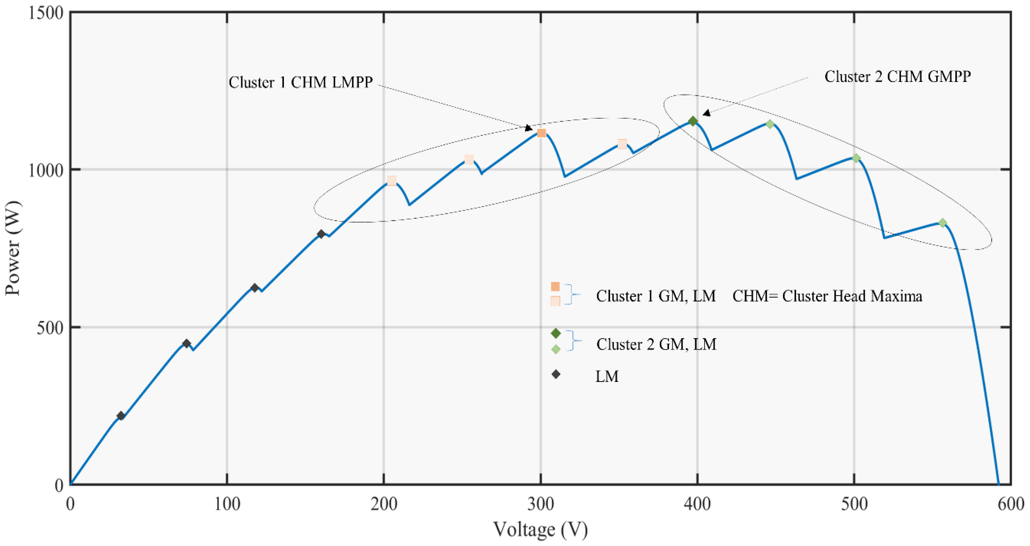
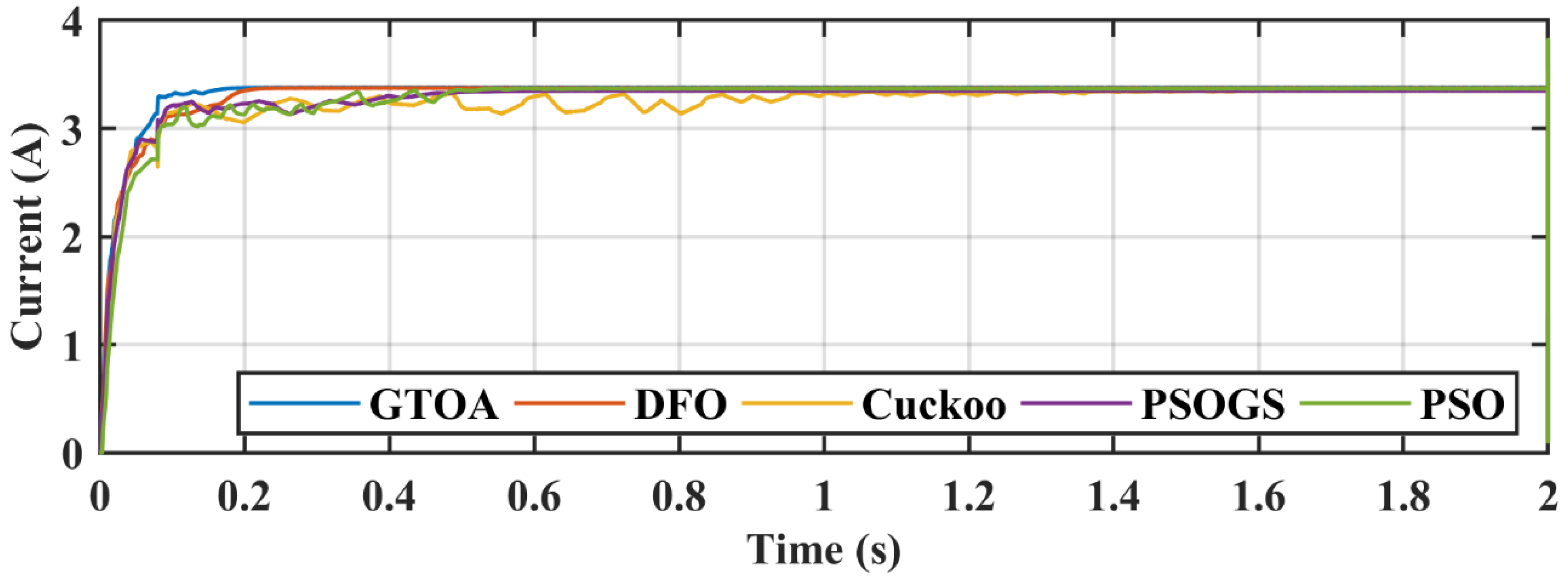
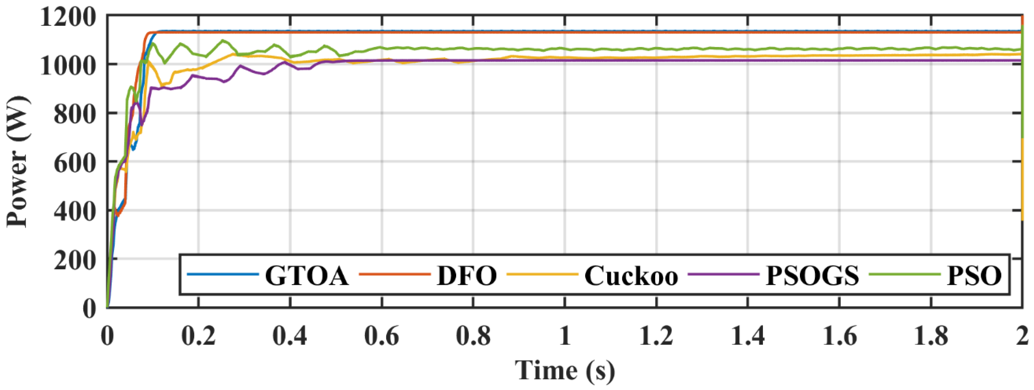
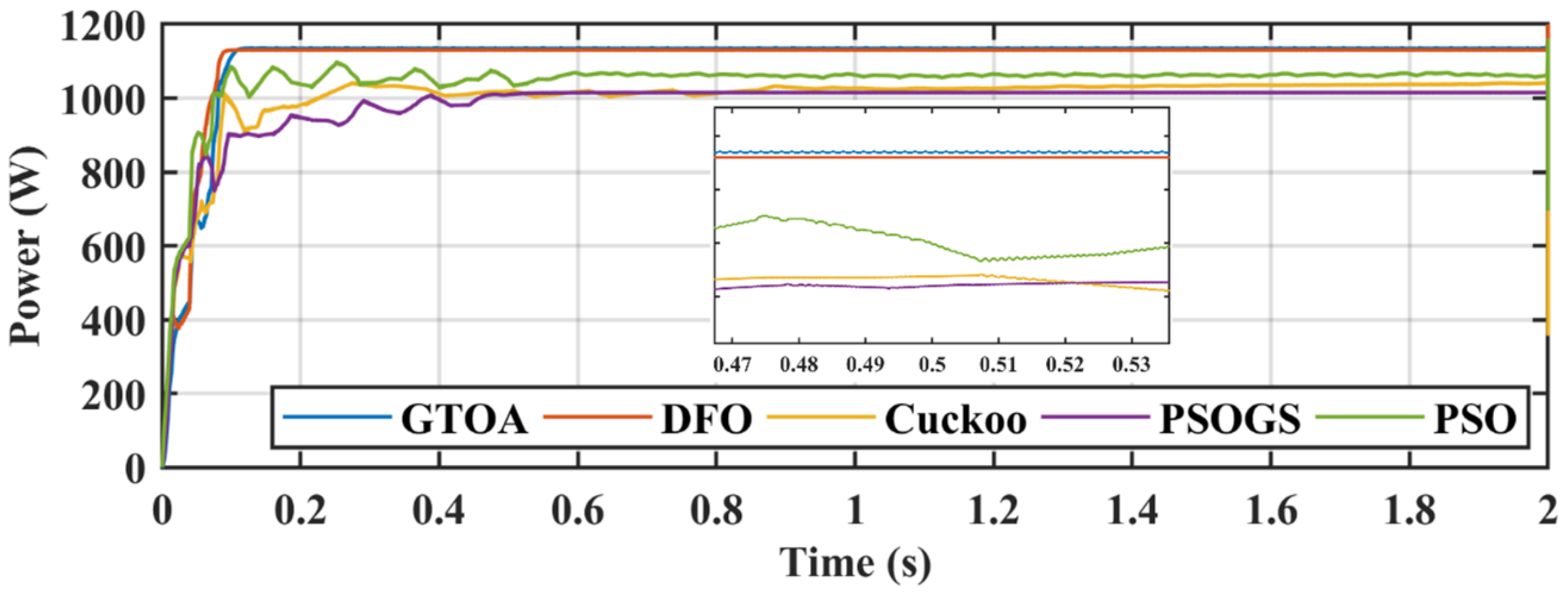
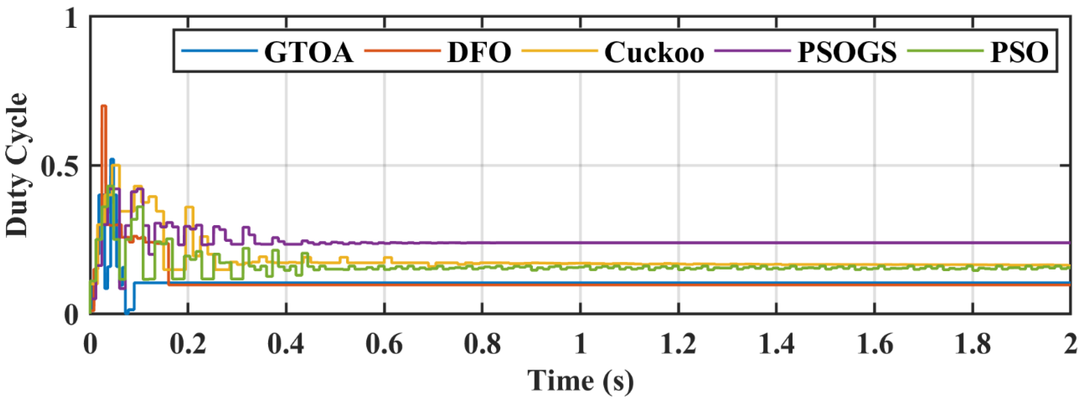
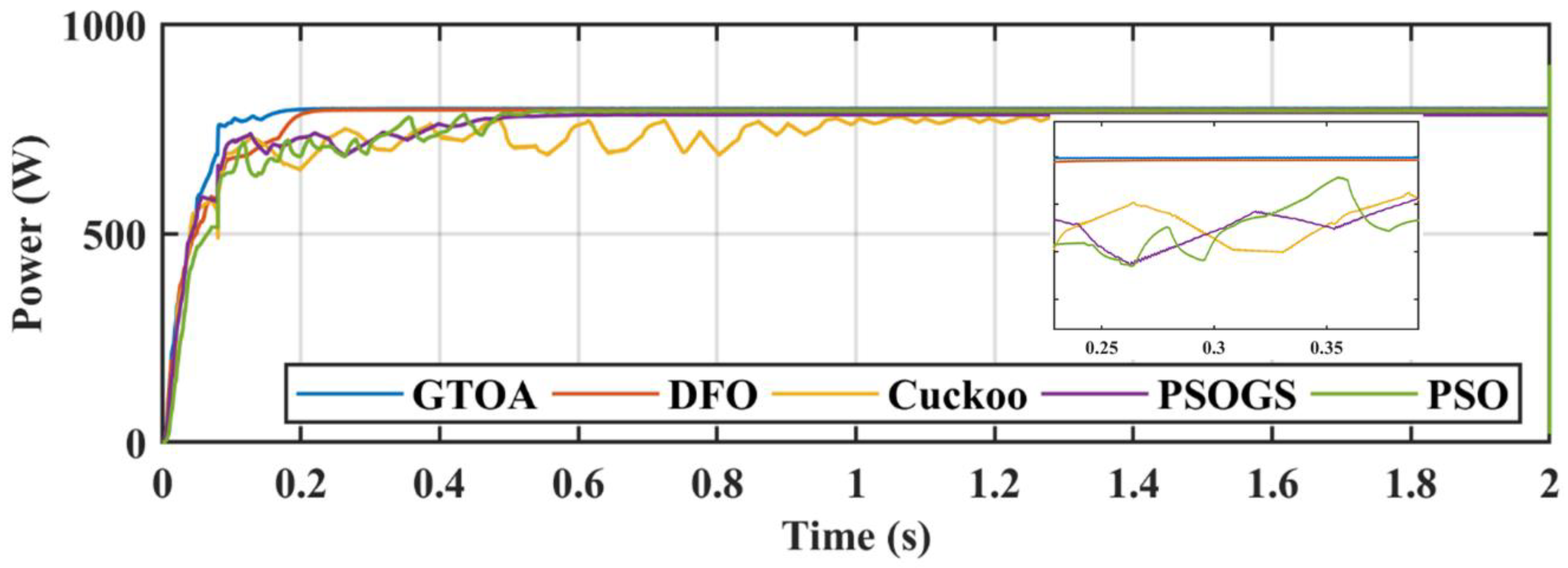
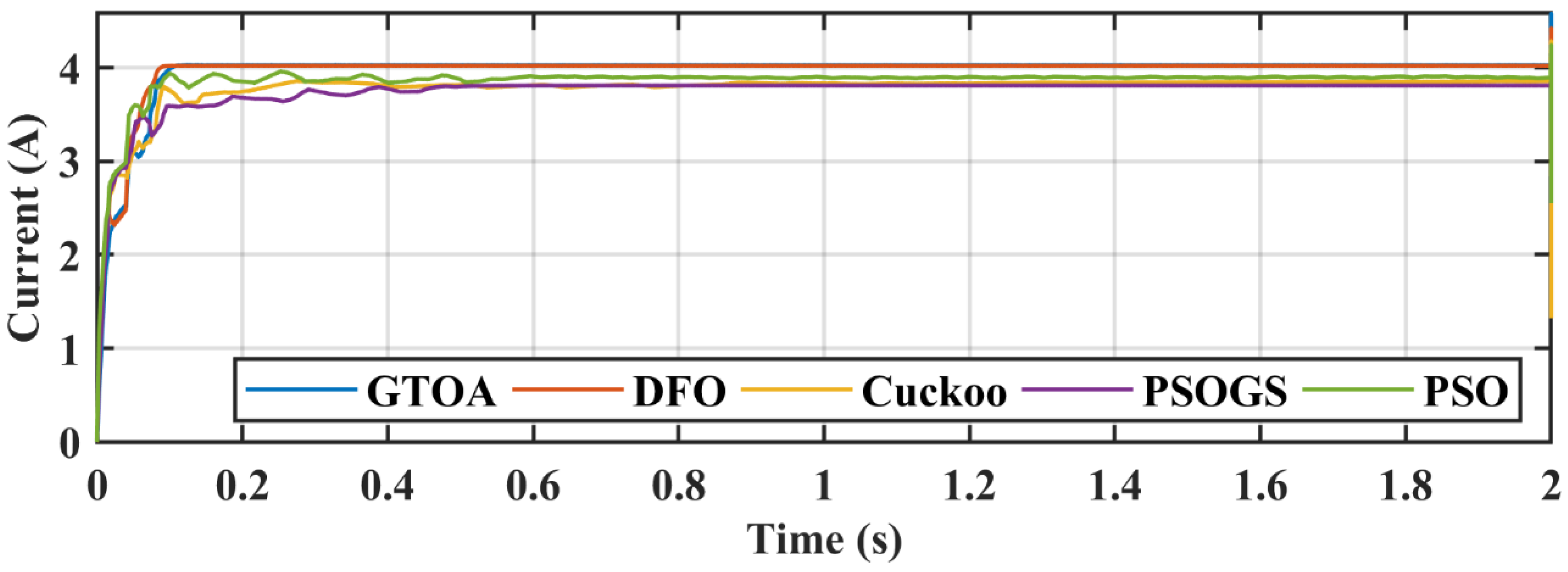
4.4. Case 4: Complex Partial Shading

CPS condition was dealt with in case 4, with 12 modules of 316 W connected in series. Irradiance levels were 350 W/m2, 250 W/m2, 310 W/m2, 180 W/m2, 370 W/m2, 450 W/m2, 490 W/m2, 570 W/m2, 650 W/m2, 600 W/m2, 750 W/m2, and 850 W/m2. Irradiance levels for all PV modules are shown in Table 3. The CPS P–V curve is explained in Figure 6, which has two clusters, and GM occurs at 1136 W. CSA and PSO trap the local maxima due to iterative decrease in velocity vectors, which reduces the exploration phase and settles at LM. PSOGS also gets trapped in LM due to the restricted movement of particles caused by the gravitational effect, which can be observed in the power comparison and the zoomed-in comparison figures, presented in Figure 27 and Figure 28, respectively. A comparison of duty cycle transients, and a zoomed-in duty cycle comparison, are presented in Figure 29 and Figure 30, respectively, and which show the exploration and exploitation behavior of GTOA in CPS conditions.
The power achieved by GTOA, DFO, CS, PSO, and PSOGS was 1135.1 W, 1131 W, 1034.8 W, 1065 W, and 1041 W, respectively, with an efficiency of 99.91%, 99.55%, 91.09%, 93.75%, and 91.63%. Convergence times of GTOA, DFO, CS, PSO, and PSOGS were 0.152 s, 0.19 s, 0.29 s, 0.32 s, and 0.45 s, with settling times of 0.23 s, 0.24 s, 0.8 s, 0.61 s, and 0.6 s. Voltage and current transient comparisons are shown in Figure 31 and Figure 32.

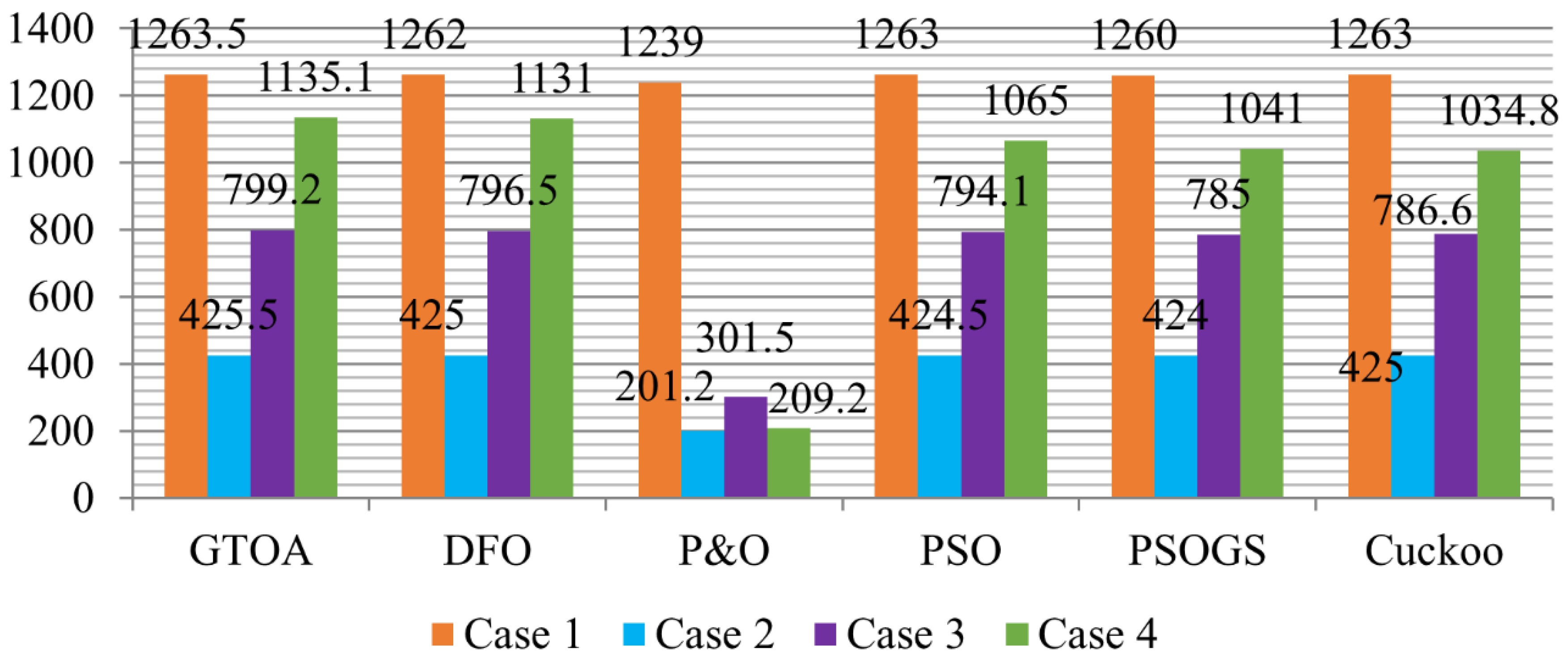
4.5. Efficiency and Performance Evaluation

Table 4 shows the comparative analysis of the MPPT techniques, which shows that GTOA mitigates the drawbacks of conventional and SI based MPPT techniques; which are oscillations around GM, trapping of LM, and high tracking time. The oscillations of GTOA around GM was less than 0.5 W , which is 97.9% less than P&O. Tracking and settling time also exhibited the performance of the MPPT technique. GTOA tracked the GM in 140 ms , and settled within 230 ms . On average GTOA was 13% to 35% faster in tracking the GM.

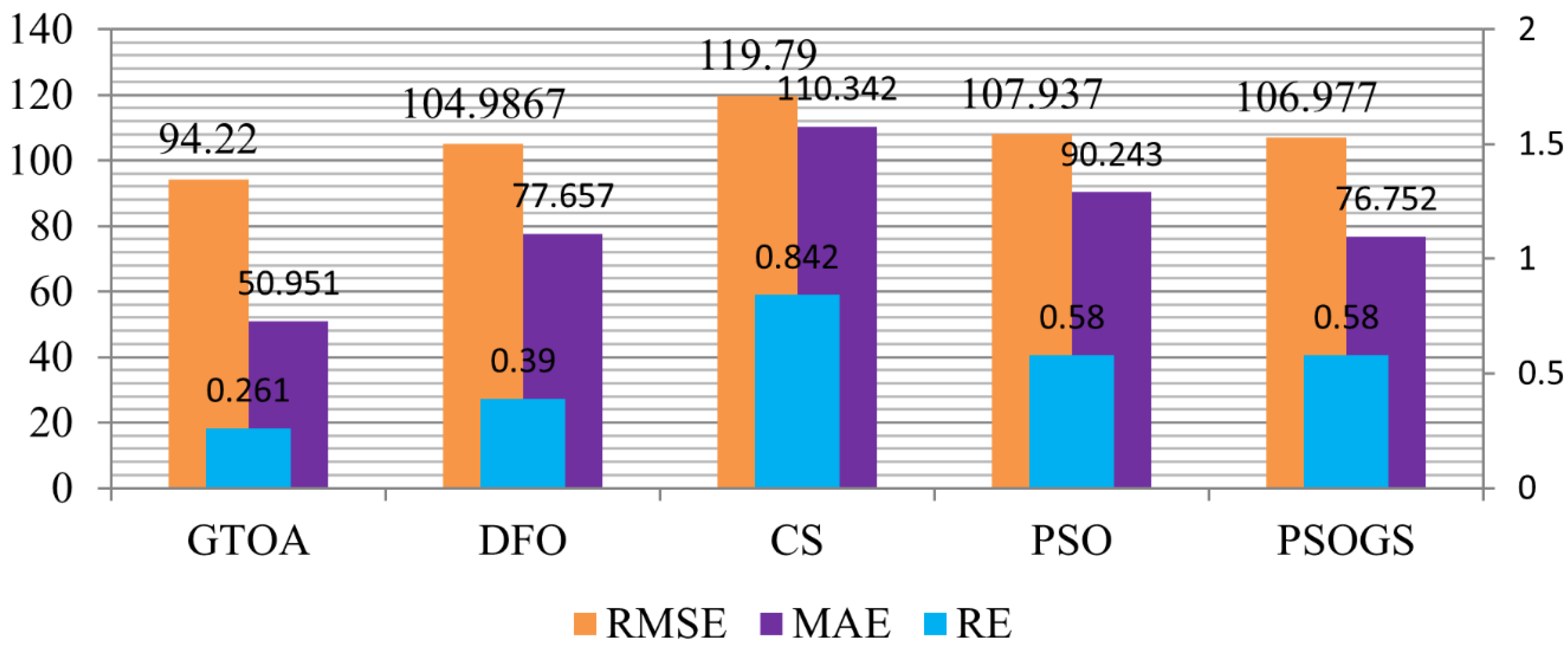
Statistical Analysis

In this section statistical analysis of GTOA is presented, in Figure 33. The sensitivity of techniques was inspected by mean absolute error (MAE) in Equation (15), relative error (RE) in Equation (14), and root means square error (RMSE) in Equation (16). STC values of the PV modules were tested against the values given in the datasheet to test the standard. Standard errors indicated that the performance of the proposed GTOA technique in the transient, as well as steady state, had a higher success rate, which indicated the effective detection of GM under all conditions.
R E = i = 1 n ( P p v i P p v ) P p v 100 %
M A E = i = 1 n ( P p v i P p v ) n
R M S E = i = 1 n ( P p v i P p v ) 2 n
where Ppvi represents the power of the panel at STC, Ppv represents tracked power, and n represents the number of samples. Figure 33 presents RMSE, MAE, and RE. Average power is given in Appendix C.

5. Conclusions

A novel GTOA based MPPT control technique is presented in this paper. This technique was experimentally evaluated against well-known P&O, DFO, PSO, PSOGS, and CS technology. The experimental simulation was carried out in five cases. Rapidly changing irradiance and PS conditions were studied. Cases 2 and 3 for PS condition, and special case 4 for complex partial shading were included. The experimental results, analysis results, and statistical analysis results showed that the proposed method has strong robustness, and is superior to competitive technology in tracking time, settling time, power tracking efficiency, and oscillation reduction. Compared with DFO, PSOGS, PSO, CS, and P&O technology, the proposed GTOA technology could track GMPP within 140 ms , while the settling time of the GTOA against competing techniques was almost 14% faster. The power efficiency of the GTOA was greater than 99.9%. Compared with other SI techniques, the average increase was 5%, however as compared to P&O it increased by 46% under PS. Overshoot, oscillation reduction, and robustness are the promising characteristics of the proposed GTOA technique. The GTOA showed significant efficiency and redundancy under extreme MPPT conditions. Steady-state oscillation was reduced to less than 0.5 W, and the transition from exploration to exploitation phase was very effective. The proposed GTOA successfully overcomes the deficiencies of the existing SI and classical MPPT controllers. In light of these comprehensive results and discussion, it is concluded that the proposed GTOA based control outperforms the existing techniques by a significant margin.

Author Contributions

Conceptualization, M.H.Z.; methodology, A.F.M., M.M., M.U.Q.; software, A.F.M., N.M.K., M.I.K.; validation, A.F.M., M.H.Z., M.M., M.I.K.; formal analysis, N.M.K., A.F.M., M.I.K.; investigation, N.M.K.; A.F.M., M.M., M.I.K.; resources, T.A.-s., R.A.N.; data curation, N.M.K., M.U.Q.; writing—original draft preparation, M.H.Z., N.M.K.; writing—review and editing, M.H.Z., A.F.M., M.I.K., M.U.Q.; visualization, M.I.K.; supervision, T.A.-s., R.A.N.; project administration, T.A.-s., R.A.N.; All authors have read and agreed to the published version of the manuscript.

Funding

The authors would like to extend their sincere appreciation to the researchers supporting project, Princess Nourah Bint Abdulrahman, Riyadh, Saudi Arabia.

Acknowledgments

The authors extend their sincere appreciation to the Deanship of Scientific Research at Princess Nourah Bint Abdulrahman University through Fast-track Research Funding Program.

Conflicts of Interest

The authors declare no conflict of interest.

Nomenclature

List of Abbreviation
PSPartial shading
GAGenetic algorithm
ACOAnt colony optimization
GTOAGroup teaching optimization algorithm
MPPTMaximum power point tracking
DFODragon fly optimization
PSOParticle swarm optimization
GMPPTGlobal maximum power point tracking
P&OPerturb and observe
Variables
Vout_dcConverts output voltage
Vin_dcConverts input voltage
N s Number of cells connected in series
CinInput capacitor
T Temperature of the p-n junction
L Inductance
CoutOutput capacitor
f Switching frequency
RLLoad resistance
a Diode ideality factor
d Duty cycle
I o Reverse saturation current
V r Thermal voltage of PV module
N p Number of cells connected in parallel
k Boltzmann constant = 1.38073 × 10 23   J / K
qElectron charge = 1.6022 × 10 19   C
Δ d Step change

Appendix A

Boost Converter

The boost converter acts as an interface between the photovoltaic (PV) panel and the load. The boost converter is responsible for adjusting the V r e f at global maxima (GM). Control variable d is modulated by maximum power point tracking (MPTT) control to achieve the best V r e f . The parameter d is bounder between 0 and 1. The parameters of DC boost converters are shown in Table 2 are calculated using Equations (A1)–(A8).
V o u t _ d c = V d i n d c 1 d
L = d × ( 1 d ) 2 × R L 2 × f
C i n = d 8 × f 2 × L × 0.01
C o u t = d 0.02 × f × R L
where Vout_dc is converts output voltage, Vin_dc is converts input voltage. Cin and Cout are input and output capacitances, respectively. Inductor L is dependent upon switching frequency f .

Appendix B

Implementation of Group Teaching Optimization Algorithm (GTOA) as MPPT

Step 1: Initialization of population
Initialize the maximum number of iterations and initialize the population using Equation (A5) within bounds given Equation (A6).
X i = { i = 1 , 2 , 3 , , N }
X i = L i + ( U i L i ) × r
where U is the upper boundary, L i is the lower boundary, r is a random number.
Step 2: Fitness evaluation
Compute fitness of each particle in population and select the best solution G .
Step 3: Stopping criteria:
Check if number of iteration is greater than the maximum iterations, stop algorithm and output the best solution G is governed by Equation (A7).
| P P V n e w P P V o l d | P P V o l d P P V ( % )
where P P V is the power of panel. Above condition will re-initialize the code and execute step 1.
Step 4: Teacher Allocation Phase:
Select top three best particles and calculate the Teacher T using Equation (13).
Step 5: Ability Group Phase:
Divide population in two groups depending upon fitness. Best half of the population in outstanding group X b e s t and others in average group X a v g .
Step 6: Teacher and Student phases:
For the best group Xbest, teacher phase is calculated using Equations (6)–(8) and (10). After that student phase is conducted using Equations (11) and (12).
For the average group X a v g , teacher phase is implemented using Equations (9) and (10). After that, create a new population in X b e s t . After that student phase is conducted using Equations (11) and (12). Create a new population of X a v g .
Step 7: Reconstruction of population
X b e s t and X a v g constructs a new population.
Step 8: Re-evaluation of population
Evaluate the population and select the optimal solution G and increase the current iteration by Equation (A8).
i t e r = i t e r + 1
Go to step 3 and execute.

Appendix C

Figure A1 shows the summary of tracked power by competing MPPT techniques as compared to GTOA. Highest power is achieved by the proposed MPPT controller in all case studies by effectively minimizing the tracking time and power loss caused by partial shading.
Figure A1. Power tracked by MPPT techniques in all cases.
Electronics 09 01962 g0a1

References

  1. Irena, G.E.C. Renewable Capacity Statistics 2017; International Renewable Energy Agency: Abu Dhabi, UAE, 2017. [Google Scholar]
  2. D’Adamo, I.; Gastaldi, M.; Morone, P. The post COVID-19 green recovery in practice: Assessing the profitability of a policy proposal on residential photovoltaic plants. Energy Policy 2020, 147, 111910. [Google Scholar] [CrossRef]
  3. Li, Z.; Ji, J.; Yuan, W.; Song, Z.; Ren, X.; Uddin, M.M.; Luo, K.; Zhao, X. Experimental and numerical investigations on the performance of a G-PV/T system comparing with A-PV/T system. Energy 2020, 194, 116776. [Google Scholar] [CrossRef]
  4. Aziz, A.S.; Tajuddin, M.F.N.; Adzman, M.R.; Mohammed, M.F.; Ramli, M.A. Feasibility analysis of grid-connected and islanded operation of a solar PV microgrid system: A case study of Iraq. Energy 2020, 191, 116591. [Google Scholar] [CrossRef]
  5. Mirza, A.F.; Mansoor, M.; Ling, Q. A novel MPPT technique based on Henry gas solubility optimization. Energy Convers. Manag. 2020, 225, 113409. [Google Scholar] [CrossRef]
  6. Eltamaly, A.M.; Farh, H.M.H. Dynamic global maximum power point tracking of the PV systems under variant partial shading using hybrid GWO-FLC. Sol. Energy 2019, 177, 306–316. [Google Scholar] [CrossRef]
  7. Mirza, A.F.; Ling, Q.; Javed, M.Y.; Mansoor, M. Novel MPPT techniques for photovoltaic systems under uniform irradiance and Partial shading. Sol. Energy 2019, 184, 628–648. [Google Scholar] [CrossRef]
  8. Tavakoli, A.; Forouzanfar, M. A self-constructing Lyapunov neural network controller to track global maximum power point in PV systems. Int. Trans. Electr. Energy Syst. 2020, 30, e12391. [Google Scholar] [CrossRef]
  9. Javed, M.Y.; Mirza, A.F.; Hasan, A.; Rizvi, S.T.H.; Ling, Q.; Gulzar, M.M.; Safder, M.U.; Mansoor, M. A Comprehensive Review on a PV Based System to Harvest Maximum Power. Electronics 2019, 8, 1480. [Google Scholar] [CrossRef] [Green Version]
  10. Ammar, H.H.; Azar, A.T.; Shalaby, R.; Mahmoud, M.I. Metaheuristic optimization of fractional order incremental conductance (FO-INC) maximum power point tracking (MPPT). Complexity 2019, 2019, 1–13. [Google Scholar] [CrossRef]
  11. Lappalainen, K.; Valkealahti, S. Number of maximum power points in photovoltaic arrays during partial shading events by clouds. Renew. Energy 2020, 152, 812–822. [Google Scholar] [CrossRef]
  12. Melhem, M. Analyzing and modeling PV with “P&O” MPPT Algorithm by MATLAB/SIMULINK. In Proceedings of the IEEE 3rd International Symposium on Small-Scale Intelligent Manufacturing Systems (SIMS), Gjøvik, Norway, 10–12 June 2020. [Google Scholar]
  13. Refaat, A.; Osman, M.H.; Korovkin, N.V. Current collector optimizer topology to extract maximum power from non-uniform aged PV array. Energy 2020, 195, 116995. [Google Scholar] [CrossRef]
  14. Ravyts, S.; Dalla Vecchia, M.; Van den Broeck, G.; Yordanov, G.H.; Gonçalves, J.E.; Moschner, J.D.; Saelens, D.; Driesen, J. Embedded BIPV module-level DC/DC converters: Classification of optimal ratings. Renew. Energy 2020, 146, 880–889. [Google Scholar] [CrossRef]
  15. Pathak, D.; Sagar, G.; Gaur, P. An Application of Intelligent Non-linear Discrete-PID Controller for MPPT of PV System. Procedia Comput. Sci. 2020, 167, 1574–1583. [Google Scholar] [CrossRef]
  16. Motahhir, S.; El Hammoumi, A.; El Ghzizal, A. The most used MPPT algorithms: Review and the suitable low-cost embedded board for each algorithm. J. Clean. Prod. 2020, 246, 118983. [Google Scholar] [CrossRef]
  17. Renaudineau, H.; Donatantonio, F.; Fontchastagner, J.; Petrone, G.; Spagnuolo, G.; Martin, J.P.; Pierfederici, S. A PSO-based global MPPT technique for distributed PV power generation. IEEE Trans. Ind. Electron. 2014, 62, 1047–1058. [Google Scholar] [CrossRef]
  18. Ishaque, K.; Salam, Z.; Amjad, M.; Mekhilef, S. An improved particle swarm optimization (PSO)-based MPPT for PV with reduced steady-state oscillation. IEEE Trans. Power Electron. 2012, 27, 3627–3638. [Google Scholar] [CrossRef]
  19. Soufyane Benyoucef, A.; Chouder, A.; Kara, K.; Silvestre, S. Artificial bee colony based algorithm for maximum power point tracking (MPPT) for PV systems operating under partial shaded conditions. Appl. Soft Comput. 2015, 32, 38–48. [Google Scholar] [CrossRef] [Green Version]
  20. Lyden, S.; Haque, M.E. A simulated annealing global maximum power point tracking approach for PV modules under partial shading conditions. IEEE Trans. Power Electron. 2015, 31, 4171–4181. [Google Scholar] [CrossRef]
  21. Ahmed, J.; Salam, Z. A Maximum Power Point Tracking (MPPT) for PV system using Cuckoo Search with partial shading capability. Appl. Energy 2014, 119, 118–130. [Google Scholar] [CrossRef]
  22. Ma, J.; Ting, T.O.; Man, K.L.; Zhang, N.; Guan, S.U.; Wong, P.W. Parameter estimation of photovoltaic models via cuckoo search. J. Appl. Math. 2013, 2013. [Google Scholar] [CrossRef]
  23. Priyadarshi, N.; Ramachandaramurthy, V.K.; Padmanaban, S.; Azam, F. An ant colony optimized MPPT for standalone hybrid PV-wind power system with single Cuk converter. Energies 2019, 12, 167. [Google Scholar] [CrossRef] [Green Version]
  24. Bouakkaz, M.S.; Boukadoum, A.; Boudebbouz, O.; Fergani, N.; Boutasseta, N.; Attoui, I.; Bouraiou, A.; Necaibia, A. Dynamic performance evaluation and improvement of PV energy generation systems using Moth Flame Optimization with combined fractional order PID and sliding mode controller. Sol. Energy 2020, 199, 411–424. [Google Scholar] [CrossRef]
  25. Mohanty, S.; Subudhi, B.; Ray, P.K. A new MPPT design using grey wolf optimization technique for photovoltaic system under partial shading conditions. IEEE Trans. Sustain. Energy 2015, 7, 181–188. [Google Scholar] [CrossRef]
  26. Javed, M.Y.; Murtaza, A.F.; Ling, Q.; Qamar, S.; Gulzar, M.M. A novel MPPT design using generalized pattern search for partial shading. Energy Build. 2016, 133, 59–69. [Google Scholar] [CrossRef]
  27. Mansoor, M.; Mirza, A.F.; Ling, Q. Harris hawk optimization-based MPPT control for PV Systems under Partial Shading Conditions. J. Clean. Prod. 2020, 274, 122857. [Google Scholar] [CrossRef]
  28. Feroz Mirza, A.; Mansoor, M.; Ling, Q.; Khan, M.I.; Aldossary, O.M. Advanced Variable Step Size Incremental Conductance MPPT for a Standalone PV System Utilizing a GA-Tuned PID Controller. Energies 2020, 13, 4153. [Google Scholar] [CrossRef]
  29. Mirza, A.F.; Mansoor, M.; Ling, Q.; Yin, B.; Javed, M.Y. A Salp-Swarm Optimization based MPPT technique for harvesting maximum energy from PV systems under partial shading conditions. Energy Convers. Manag. 2020, 209, 112625. [Google Scholar] [CrossRef]
  30. Mansoor, M.; Mirza, A.F.; Ling, Q.; Javed, M.Y. Novel Grass Hopper optimization based MPPT of PV systems for complex partial shading conditions. Sol. Energy 2020, 198, 499–518. [Google Scholar] [CrossRef]
  31. Zhang, Y.; Jin, Z. Group teaching optimization algorithm: A novel metaheuristic method for solving global optimization problems. Expert Syst. Appl. 2020, 148, 113246. [Google Scholar] [CrossRef]
Figure 1. A photovoltaic (PV) system with maximum power point tracking (MPPT) control.
Electronics 09 01962 g001
Figure 2. Single diode model of a PV cell.
Electronics 09 01962 g002
Figure 3. (a) Under uniform irradiance I–V curves. (b) Under uniform irradiance P–V curves. (c) Under non-uniform irradiance I–V curves. (d) Under non-uniform irradiance P–V curves.
Electronics 09 01962 g003
Figure 4. PV array in series-parallel combination with bypass and blocking diodes, under uniform and non-uniform irradiance.
Electronics 09 01962 g004
Figure 5. Phases for implementation of the group teaching optimization algorithm (GTOA).
Electronics 09 01962 g005
Figure 6. Formation of the cluster in complex partial shading conditions.
Electronics 09 01962 g006
Figure 7. Tracking mechanism of GTOA under partial shading (PS) conditions.
Electronics 09 01962 g007
Figure 8. Working of GTOA as MPPT under PS conditions.
Electronics 09 01962 g008
Figure 9. Comparison of power of GTOA. Dragon fly optimization (DFO), particle swarm optimization (PSO), perturb and observe (P&O), and particle swarm optimization gravitational search (PSOGS).
Electronics 09 01962 g009
Figure 10. Zoomed-in comparison of power of GTOA.
Electronics 09 01962 g010
Figure 11. Comparison of duty cycle of GTOA.
Electronics 09 01962 g011
Figure 12. Zoomed-in comparison of duty cycle of GTOA.
Electronics 09 01962 g012
Figure 13. Comparison of voltage transients of GTOA.
Electronics 09 01962 g013
Figure 14. Comparison of current transients of GTOA.
Electronics 09 01962 g014
Figure 15. Comparison of power of GTOA.
Electronics 09 01962 g015
Figure 16. Zoomed-in comparison of power of GTOA.
Electronics 09 01962 g016
Figure 17. Comparison of duty cycle of GTOA.
Electronics 09 01962 g017
Figure 18. Zoomed-in comparison of duty cycle of GTOA.
Electronics 09 01962 g018
Figure 19. Comparison of voltage transients of GTOA.
Electronics 09 01962 g019
Figure 20. Comparison of current transients of GTOA.
Electronics 09 01962 g020
Figure 21. Comparison of power of GTOA.
Electronics 09 01962 g021
Figure 22. Zoomed-in comparison of power of GTOA.
Electronics 09 01962 g022
Figure 23. Comparison of duty cycle of GTOA.
Electronics 09 01962 g023
Figure 24. Zoomed-in comparison of duty cycle of GTOA.
Electronics 09 01962 g024
Figure 25. Comparison of voltage transients of GTOA.
Electronics 09 01962 g025
Figure 26. Comparison of current transients of GTOA.
Electronics 09 01962 g026
Figure 27. Comparison of power of GTOA.
Electronics 09 01962 g027
Figure 28. Zoomed-in comparison of power of GTOA.
Electronics 09 01962 g028
Figure 29. Comparison of duty cycle of GTOA.
Electronics 09 01962 g029
Figure 30. Zoomed-in comparison of duty cycle of GTOA.
Electronics 09 01962 g030
Figure 31. Comparison of voltage transients of GTOA.
Electronics 09 01962 g031
Figure 32. Comparison of current transients of GTOA.
Electronics 09 01962 g032
Figure 33. Comparative analysis of root means square error (RMSE), mean absolute error (MAE), and relative error (RE).
Electronics 09 01962 g033
Table 1. Electrical parameters of the “Sunpreme SNPM-GX-315”.
Maximum Power Pmpp316 W
Short Circuit Voltage Voc51.1 V
Voltage at MP Vmpp39.5 V
Short Circuit Current Isc8.5 A
Current at MP Impp8 A
No. of Cells Ns72
Shunt resistance805.8807 Ω
Series resistance0.6912 Ω
Table 2. Irradiance pattern PS condition.
Case Study Irradiances   ( G )   of   Each   PV   Module   ( K W m 2 ) Pmax (Watts)
PV1PV2PV3PV4
Case 11,000,400,7501,000,450,7501,000,400,7501,000,400,7501,264,530,970
Case 2650520250400427
Case 37201000850550799.8
Table 3. Irradiance pattern for CPS.
Case Irradiance   S i   ( K W m 2 ) Pmax
Case 4PV1:350PV5:370PV9:650Pmax = 1136 W
PV2:250PV6:450PV10:600
PV3:310PV7:490PV11:750
PV4:180PV8:570PV12:850
Table 4. Quantitative analysis of GTOA with dragon fly optimization (DFO), particle swarm optimization (PSO), perturb and observe (P&O), cuckoo search (CS), and particle swarm optimization gravitational search (PSOGS).
Tech.
Technique
Case No.Convergence Time (s)Settling Time (s)GM LocatedPower at GM (W)Power Tracked (W)Effie.
(%)
GTOACase 10.1350.220Yes12641263.599.96
Case 20.1450.225Yes427425.599.85
Case 30.1480.250Yes800799.299.92
Case 40.1520.23Yes11361135.199.97
DFOCase 10.1550.240Yes1264126299.84
Case 20.1860.238Yes42742599.64
Case 30.2050.26Yes800796.599.58
Case 40.1900.24Yes1136113199.93
P & OCase 10.100.10Yes1264123998.02
Case 2LMLMNo427201.247.11
Case 3LMLMNo800301.537.68
Case 4LMLMNo1136209.218.45
PSOCase 10.410.90Yes1264126399.92
Case 20.490.90Yes427424.599.39
Case 30.300.57Yes800794.199.30
Case 40.320.61No1136106593.75
PSOGSCase 10.340.62Yes1264126099.68
Case 20.350.59Yes42742499.29
Case 30.390.60Yes80078598.14
Case 40.450.60No1136104191.63
CSCase 10.310.71Yes1264126399.92
Case 20.270.69Yes42742599.57
Case 30.451.20Yes800786.698.34
Case 40.290.80No11361034.891.09
Publisher’s Note: MDPI stays neutral with regard to jurisdictional claims in published maps and institutional affiliations.

