Simplification on Cross-Component Linear Model in Versatile Video Coding

Abstract

To improve coding efficiency by exploiting the local inter-component redundancy between the luma and chroma components, the cross-component linear model (CCLM) is included in the versatile video coding (VVC) standard. In the CCLM mode, linear model parameters are derived from the neighboring luma and chroma samples of the current block. Furthermore, chroma samples are predicted by the reconstructed samples in the collocated luma block with the derived parameters. However, as the CCLM design in the VVC test model (VTM)-6.0 has many conditional branches in its processes to use only available neighboring samples, the CCLM implementation in parallel processing is limited. To address this implementation issue, this paper proposes including the neighboring sample generation as the first process of the CCLM, so as to simplify the succeeding CCLM processes. As unavailable neighboring samples are replaced with the adjacent available samples by the proposed CCLM, the neighboring sample availability checks can be removed. This results in simplified downsampling filter shapes for the luma sample. Therefore, the proposed CCLM can be efficiently implemented by employing parallel processing in both hardware and software implementations, owing to the removal of the neighboring sample availability checks and the simplification of the luma downsampling filters. The experimental results demonstrate that the proposed CCLM reduces the decoding runtime complexity of the CCLM mode, with negligible impact on the Bjøntegaard delta (BD)-rate.

1. Introduction

After decades of development of international video coding standards by the collaborative efforts of the ITU-T WP3/16 Video Coding Experts Group (VCEG) and the ISO/IEC JTC 1/SC 29/WG 11 Moving Picture Experts Group (MPEG), video coding technology has achieved tremendous progress in its compression capability. As the recent demand for high resolution and high quality video contents by end-users has increased in application areas such as video streaming, video conferencing, remote screen sharing, and cloud gaming, the industry needs more efficient video coding technology to further reduce the network bandwidth or storage requirements of video content. To respond to such needs from the industry, the state-of-the-art VVC standard [1] was developed by the Joint Video Experts Team (JVET) of the VCEG and the MPEG, and finalized in July 2020. VVC is the successor to block-based hybrid video codecs such as the Advanced Video Coding (AVC) standard [2,3] and the High Efficiency Video Coding (HEVC) standard [4,5], and provides coding efficiency improvements of approximately 40% [6] over HEVC for ultra high definition (UHD) test sequences, in terms of the objective video quality measure of Bjøntegaard delta (BD)-rate [7,8]. The main target application areas for VVC include UHD video, high dynamic range (HDR), and wide color gamut (WCG) video, screen content video, and 360° omni-directional video, as well as conventional standard definition (SD) and high definition (HD) videos. In the standardization of VVC, new coding tools were developed with the aim of compressing the video content by removing the intra-picture, inter-picture, and statistical redundancies within the original video signal. Among the fundamental building blocks of typical block-based hybrid video codecs, the intra prediction exploits the intra-picture redundancy by predicting samples of the current block from spatially reconstructed neighboring samples. Compared to its predecessors, to improve the coding efficiency of intra prediction, VVC includes many outstanding intra prediction coding tools, such as 67 intra prediction modes, wide angle prediction (WAP), intra prediction with multiple reference lines (MRL), intra sub-partitions (ISP), matrix-based intra prediction (MIP), CCLM intra prediction, and position-dependent prediction combination (PDPC) [9].

More specifically, the aforementioned intra prediction coding tools, except for the CCLM, reduce the spatial redundancy, which is the redundancy between the samples of spatially adjacent blocks within the picture. On the other hand, it can be shown that the CCLM exploits inter-component redundancy in a way that reduces the redundancy between the luma and chroma component samples within the picture. Typically, digital video contents acquired by digital camera sensors are composed of multiple components such as R, G, and B components in the RGB color space. To reduce the inter-component redundancy in the RGB color space, Y, Cb, and Cr components in the YCbCr color space are obtained by performing a linear color transform on the R, G, and B components. However, local signal redundancy between the components can be observed, even in the decorrelated YCbCr color space [10,11]. The local inter-component redundancy between the luma (Y) component and the chroma (Cb or Cr) component was first exploited in [12] to improve the coding efficiency of AVC. Based on [12], a chroma prediction method using inter-channel correlation [13], which was later called the CCLM, was proposed in the development of the HEVC standard. This method employed a linear model that allows the chroma samples to be predicted based on the reconstructed luma samples in the collocated block using the least mean squares (LMS) algorithm at the decoder. Although various other methods related to the CCLM were proposed to improve the coding efficiency or the implementation complexity during the HEVC standardization, the CCLM was not included in the HEVC Version 1 profiles because of its hardware implementation complexity, with regard to pipeline latency. However, a simplified method in the residual domain, called cross-component prediction (CCP) [14], which signals the slope parameter of the linear model to the decoder, was adopted into the Range Extensions (RExt) of HEVC [15]. After the HEVC standardization was finalized, the joint exploration test model (JEM) [16,17] was developed by VCEG and MPEG to study the potential need for the standardization of the next generation video coding standard, with an improved compression capability over HEVC. The CCLM was again included in JEM to evaluate its potential coding efficiency and the possibility of its future adoption in the next generation video coding standard. In the VVC standardization, based on the CCLM in JEM, plenty of proposals were investigated for enhancing the coding efficiency and the implementation complexity. With these efforts in standardization, the CCLM has become one of the most efficient intra prediction coding tools in VVC, since it achieves BD-rate savings of approximately 1.5% and 14% for the luma component and chroma components in the all intra configuration, respectively [18]. The CCLM was finally included in the VVC Version 1 profiles.

Although the CCLM achieves an impressive coding gain it is accompanied by complexities, such as pipeline latency, memory access, and computational complexity. Among these complexities, the main complexity aspect that this study focused on is the computational complexity of the CCLM. The computational complexity reduction of the CCLM mode is important to enable the real-time implementation of VVC. The purpose of this paper is to provide a methodology for reducing the computational complexity of the CCLM, and achieving the real-time encoding and decoding of VVC. Specifically, the CCLM design in the VTM-6.0 reference software [19] has many conditional branches in its processes to use only available neighboring samples; thus, there is a limitation on the implementation of the CCLM using parallel processing, such as single instruction multiple data (SIMD). To address the aforementioned implementation issue, the proposed CCLM is motivated by the assumption that if all of the neighboring samples are available, the succeeding processes in the CCLM can be simplified. Therefore, in this study, the neighboring sample generation process is added as the first process into the CCLM processes, to simplify the succeeding processes in the CCLM. In the proposed CCLM, as all of the neighboring samples are made available by the neighboring sample generation process already specified in VVC, the conditional branches restricting the usage of parallel processing can be removed. As a result, especially for the downsampling filters for the luma sample, a simplified downsampling filter shape is achieved. Fixed subsampled neighboring sample positions for the derivation of linear model parameters are also achieved. Thus, by simply adding the neighboring sample generation process into the CCLM mode in VVC, the CCLM mode can be efficiently implemented by employing parallel processing, thereby achieving cost-effective implementation of the video coding technology, which is an essential application in the signal processing field. It should be noted that the method presented in this paper was also proposed in the 15th and 16th JVET meetings [20,21]. Afterwards, a repetitive padding method of the luma samples for the usage of the same downsampling filter [22], which is conceptually similar to the method presented in this paper, was adopted into VTM-8.0 in the 17th JVET meeting.

The remainder of this paper is structured as follows: In Section 2, a description of the CCLM in VTM-6.0 is reviewed. Next, a description of the proposed CCLM, and a comparative analysis of the CCLM design between VTM-6.0 and the proposed CCLM, are presented in Section 3. The objective BD-rate results of the proposed CCLM, on top of VTM-6.0, are provided in Section 4. Finally, Section 5 concludes the study.

2. Description of the CCLM in VTM-6.0

In VTM-6.0, when a chroma block is decoded as one of the CCLM modes, consisting of the LT_CCLM, T_CCLM, and L_CCLM modes [23,24], the linear model parameters are derived at the decoder from the reconstructed neighboring luma and chroma samples of the current block using the equation of the straight line. Then, the chroma samples in the current block are predicted by the downsampled reconstructed samples in the collocated luma block with the derived linear model parameters. 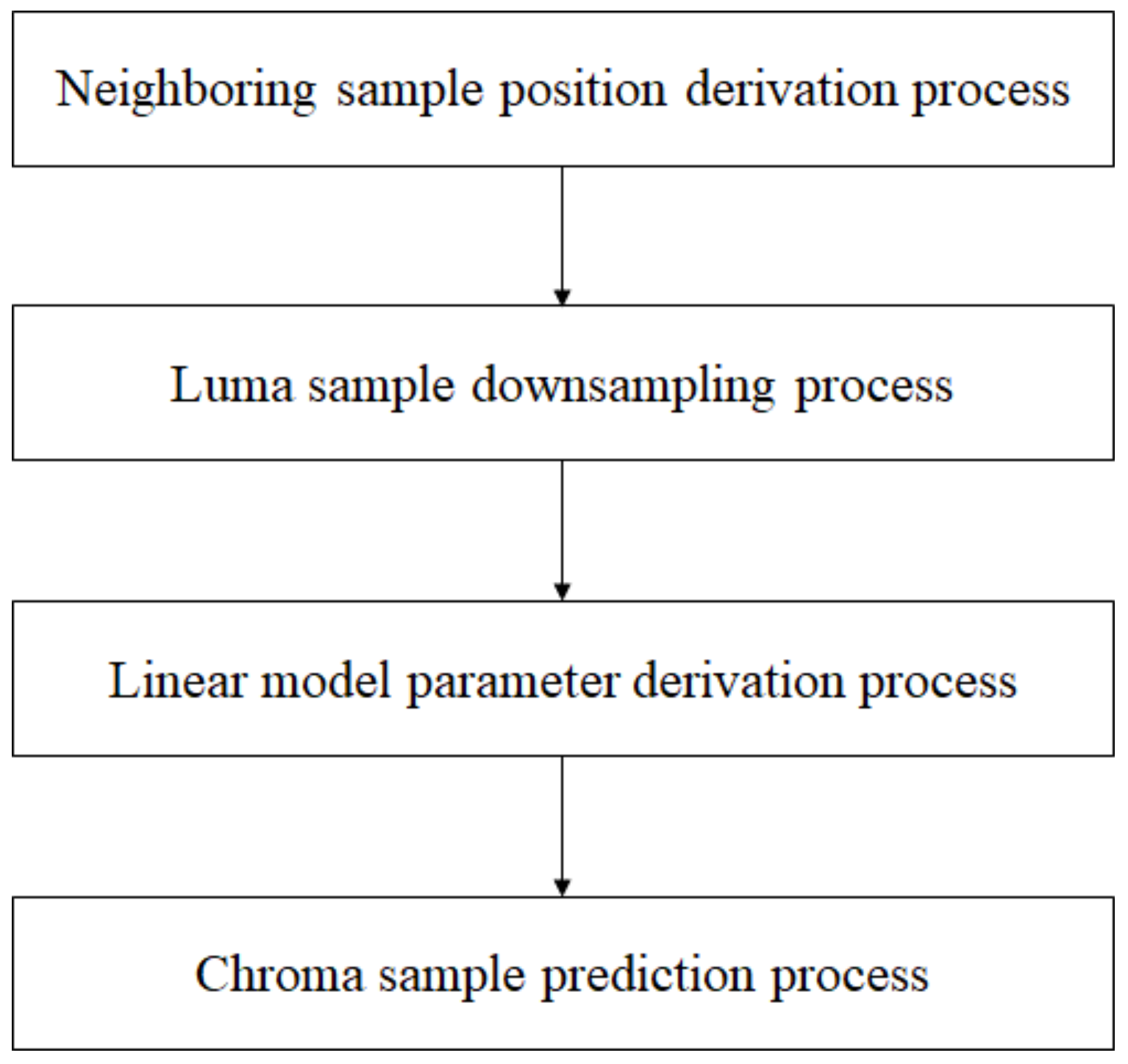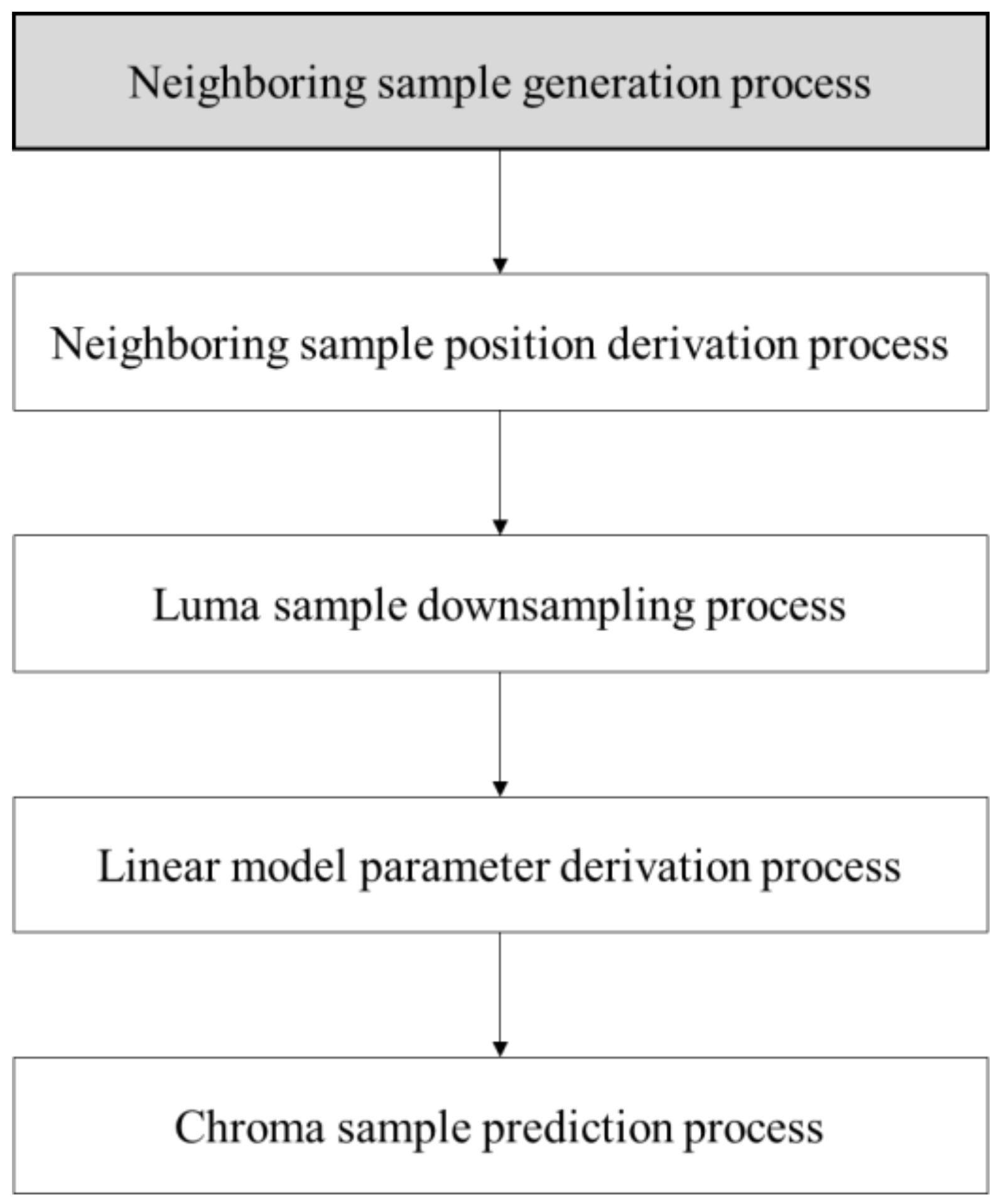Figure 1 shows the processing flow chart of the CCLM in VTM-6.0. As shown in the figure, the CCLM is composed of the neighboring sample position derivation process, the luma sample downsampling process, the linear model parameter derivation process, and the chroma sample prediction process. More specifically, each process of the CCLM is described as follows.

First, the positions for the reconstructed neighboring chroma samples and their corresponding reconstructed neighboring luma samples are derived in the neighboring sample position derivation process. Suppose the dimensions of the current chroma block are W_C × H_C, then the number of available top and top-right neighboring chroma samples (W_{C_A}) and the number of available left and left-below neighboring chroma samples (H_{C_A}) are derived as in Equations (1) and (2):

$$W_{C\_A}= \left\{\begin{array}{c}{W}_C \mathrm{for} \mathrm{L}\mathrm{T}\_\mathrm{C}\mathrm{C}\mathrm{L}\mathrm{M} \mathrm{mode}\\ W_C+\min \left(N_{TR}, H_C\right) \mathrm{for} \mathrm{T}\_\mathrm{C}\mathrm{C}\mathrm{L}\mathrm{M} \mathrm{mode} \end{array}\right.$$

(1)

$$H_{C\_A}= \left\{\begin{array}{c}{H}_C \mathrm{for} \mathrm{L}\mathrm{T}\_\mathrm{C}\mathrm{C}\mathrm{L}\mathrm{M} \mathrm{mode}\\ H_C+\min \left(N_{LB},W_C\right) \mathrm{for} \mathrm{L}\_\mathrm{C}\mathrm{C}\mathrm{L}\mathrm{M} \mathrm{mode} \end{array}\right.$$

(2)

where N_TR and N_LB represent the number of available top-right neighboring chroma samples and the number of available left-below neighboring chroma samples, respectively. As can be seen from Equations (1) and (2), for the T_CCLM and L_CCLM modes, W_{C_A} and H_{C_A} are derived based on N_TR and N_LB, which require checking of the top-right and left-below neighboring sample availabilities, respectively. Here, for example, the neighboring sample is considered as available when the neighboring sample exists in the same picture, slice, or tile where the current block belongs. As proposed in [25,26], from the available top and top-right neighboring chroma samples, R_C (0, −1) to R_C(W_{C_A} − 1, −1), and the available left and left-below neighboring chroma samples, R_C (−1, 0) to R_C (−1, H_{C_A} − 1), up to four neighboring chroma samples are selected by subsampling the neighboring sample positions as

• R_C(W_{C_A}/4, −1), R_C(3 × W_{C_A}/4, −1), R_C(−1, H_{C_A}/4), R_C(−1, 3 × H_{C_A}/4) for the LT_CCLM mode
• R_C(W_{C_A}/8, −1), R_C(3 × W_{C_A}/8, −1), R_C(5 × W_{C_A}/8, −1), R_C(7 × W_{C_A}/8, −1) for the T_CCLM mode
• R_C(−1, H_{C_A}/8), R_C(−1, 3 × H_{C_A}/8), R_C(−1, 5 × H_{C_A}/8), R_C(−1, 7 × H_{C_A}/8) for the L_CCLM mode

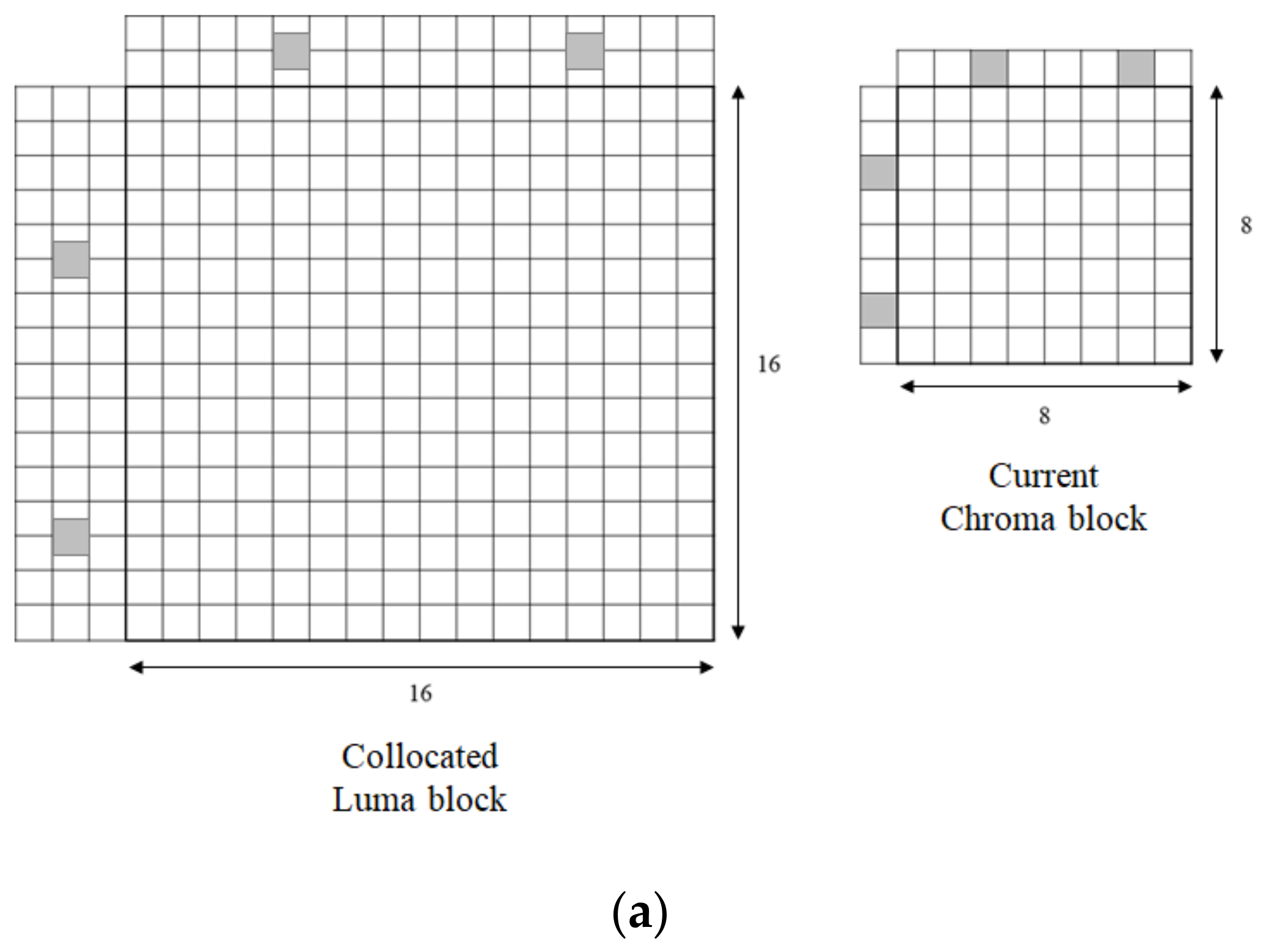
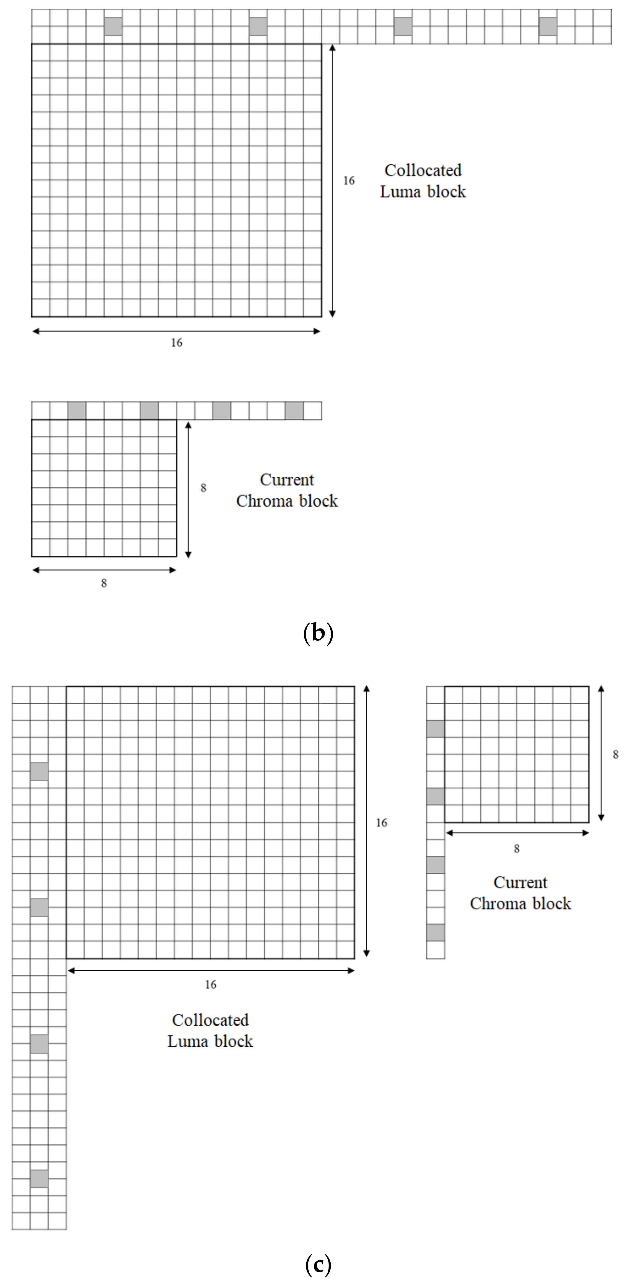
Here, R_C(i, j) indicates the reconstructed chroma sample at coordinates (i, j) and R_C(0, 0) indicates the top-left reconstructed chroma sample of the current chroma block. The subsampled neighboring chroma sample positions are used to derive the corresponding subsampled neighboring luma sample positions based on the chroma subsampling ratio. Figure 2 illustrates examples of the subsampled neighboring chroma sample positions and the corresponding subsampled neighboring luma sample positions for the LT_CCLM, T_CCLM, and L_CCLM modes, when the chroma subsampling ratio is 4:2:0. In the figure, the square boxes indicate the sample positions, the shaded boxes represent the subsampled sample positions for the neighboring samples of the current 8 × 8 chroma block and the neighboring samples of the corresponding 16 × 16 luma block, and the sample positions outside the blocks are the available neighboring sample positions.

Second, in the luma sample downsampling process, the downsampled neighboring luma samples and the downsampled collocated luma samples are derived by downsampling the luma samples at the subsampled neighboring sample positions, and in the collocated luma block, according to the chroma subsampling ratio, respectively. For the chroma subsampling ratio of 4:2:0 or 4:2:2, the neighboring and collocated luma samples are downsampled before the linear model parameter derivation according to the chroma sample location. Basically, two different downsampling filter shapes, which are rectangular-shaped filters with filter coefficients of (1, 2, 1, 1, 2, 1) and a cross-shaped filter with filter coefficients of (1, 1, 4, 1, 1), are used for downsampling of the neighboring and collocated luma samples, depending on the chroma sample location type-0 and type-2 [27]. Here, high-level information, called sps_cclm_colocated_chroma_flag, is signaled to the decoder to indicate the chroma sample location type. The downsampling filter shapes are further modified based on the neighboring sample availability, the sample position within the block, the subsampled neighboring sample position, and the coding tree unit (CTU) boundary condition. Here, to reduce the line buffer requirement at the top CTU boundary, only one top neighboring luma sample line is used for the derivation of the linear model parameters [28,29].

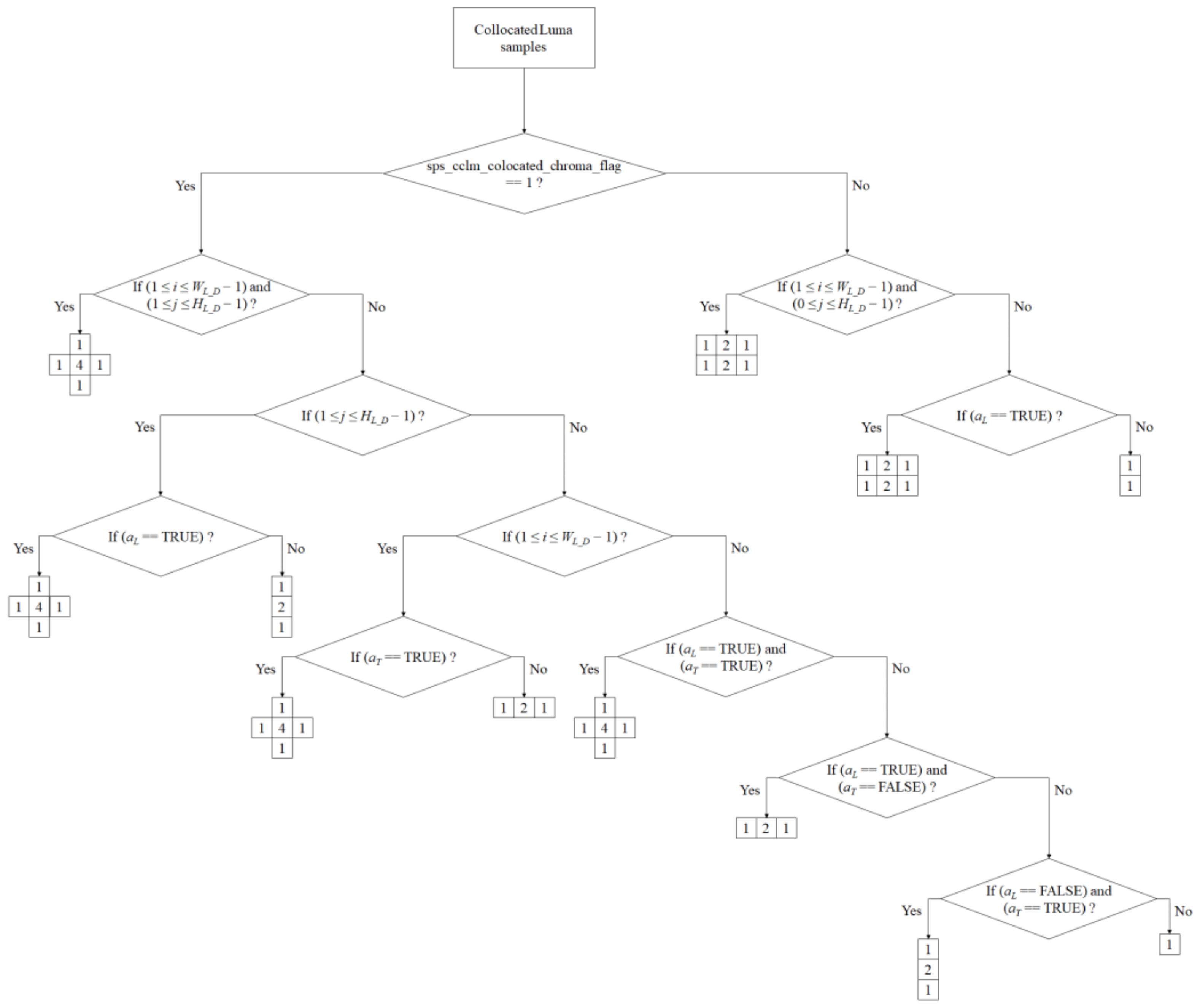
Figure 3 illustrates the flow chart of downsampling filter shape selection for the collocated luma samples, depending on the various conditions with respect to sps_cclm_colocated_chroma_flag, the sample positions within the block, and the neighboring sample availabilities. In the figure, W_{L_D} and H_{L_D} represent the width and height of the downsampled collocated luma block, respectively; a_T and a_L indicate the top and left neighboring sample availabilities, respectively; and i and j indicate the coordinates of the downsampled luma sample position in the horizontal and vertical directions within the collocated luma block, respectively. It is noted that after filtering with the downsampling filter coefficients shown in the figure, the filtering results are normalized by the sum of the filter coefficients.

Referring to Figure 4, one of the downsampling filter shapes for the top neighboring luma samples is selected based on sps_cclm_colocated_chroma_flag, the subsampled neighboring sample positions, the neighboring sample availability, and the CTU boundary condition. In the figure, a_TL indicates whether both the top and left neighboring samples are available, and the first subsampled sample position is the leftmost subsampled sample position among the four subsampled neighboring luma sample positions. The CTU boundary condition in the figure indicates if the top boundary of the current block is the CTU boundary. When this condition is met, only the nearest top neighboring luma sample line is used for downsampling of the top neighboring luma samples.

Figure 5 shows the flow chart of downsampling filter shape selection for the left neighboring luma samples, based on sps_cclm_colocated_chroma_flag, the subsampled neighboring sample positions, and the neighboring sample availability. In the figure, the first subsampled sample position indicates the topmost subsampled sample position among the four subsampled neighboring luma sample positions.

Third, using the downsampled neighboring luma samples and the subsampled neighboring chroma samples, two linear model parameters are derived in the linear model parameter derivation process. The values of four downsampled neighboring luma samples are compared to determine the two minimum luma sample values, R_{L_D_MIN0} and R_{L_D_MIN1}, and two maximum luma sample values, R_{L_D_MAX0} and R_{L_D_MAX1}. Furthermore, two minimum chroma sample values, R_{C_MIN0} and R_{C_MIN1}, and two maximum chroma sample values, R_{C_MAX0} and R_{C_MAX1}, are derived from the corresponding four neighboring chroma samples [25,26]. For the equation of the straight line, two points, which represent the luma sample values in the x-axis and the chroma sample values in the y-axis, are obtained as follows: The luma sample values of two points, denoted by X_P0 and X_P1, are derived by averaging the two minimum luma sample values, and averaging the two maximum luma sample values, as in Equations (3) and (4):

$$X_{P0}= \left(R_{L\_D\_MIN0}+R_{L\_D\_MIN1}+1\right) \gg 1$$

(3)

$$X_{P1}= \left(R_{L\_D\_MAX0}+R_{L\_D\_MAX1}+1\right) \gg 1$$

(4)

Similarly, by averaging the two minimum chroma sample values and averaging the two maximum chroma sample values, as in Equations (5) and (6), the chroma sample values of the two points, denoted by Y_P0 and Y_P1, are derived.

$$Y_{P0}= \left(R_{C\_MIN0}+R_{C\_MIN1}+1\right) \gg 1$$

(5)

$$Y_{P1}= \left(R_{C\_MAX0}+R_{C\_MAX1}+1\right) \gg 1$$

(6)

Then, as proposed in [30], the equation of the straight line connecting the obtained two points is used to derive the slope parameter, α, in Equation (7), and the y-intercept, β, is calculated using Equation (8).

$$\alpha =\frac{Y_{P1}-Y_{P0}}{X_{P1}-X_{P0}}$$

(7)

$$\beta =Y_{P0}-\alpha \times X_{P0}$$

(8)

Finally, in the chroma sample prediction process, the chroma prediction samples are obtained from the downsampled reconstructed samples in the collocated luma block using the derived linear model parameters in Equation (9).

$$P_C\left(i, j\right) =\alpha \times R_{L\_D}\left(i, j\right) + \beta$$

(9)

where P_C and R_{L_D} represent the chroma prediction sample and the downsampled reconstructed sample in the collocated luma block, respectively.

3. Proposed Method

There are dependencies on the available neighboring samples in the neighboring sample position derivation process, the luma sample downsampling process, and the linear model parameter derivation process of the CCLM in VTM-6.0. In other words, many conditional branches that use only the available neighboring samples exist in these processes. More specifically, in the neighboring sample position derivation process, up to four subsampled neighboring sample positions are derived based on W_{C_A} and H_{C_A}, which are dependent on N_TR and N_LB, respectively. Furthermore, various shapes of the downsampling filter are used in the luma sample downsampling process, where the downsampling filter selection depends on the neighboring sample availability, the sample positions within the block, the subsampled sample positions for neighboring samples, and the CTU boundary condition. Moreover, the number of subsampled neighboring samples used in the linear model parameter derivation is variable because it is also dependent on the neighboring sample availabilities. Accordingly, many conditional branches entail a burden on implementation of the CCLM, in terms of computational complexity. More precisely, checking the neighboring sample availability makes it difficult to employ parallel processing such as SIMD in software implementation, and requires many cycles and logic in hardware implementation.

To address this implementation issue, in the proposed CCLM method, the neighboring sample generation process is added to the CCLM as the first process to simplify the succeeding neighboring sample position derivation process, the luma sample downsampling process, and the linear model parameter derivation process. Figure 6 shows the processing flow chart of the proposed CCLM, where the neighboring sample generation process, already used for general intra prediction, such as 67 intra prediction modes in VVC, is performed before the neighboring sample position derivation process. In hardware implementation, the proposed CCLM can be implemented without additional logics for VVC, because the logics for the neighboring sample generation process can be shared with those used for general intra prediction. Furthermore, the proposed CCLM mode can be performed without introducing repetitive padding operations, which has an advantage over [22] in terms of the implementation complexity.

In the proposed CCLM, the neighboring sample generation process makes all of the neighboring samples available to remove the conditional branches, restricting the usage of parallel processing. As a result, a simplified downsampling filter shape is achieved in the luma sample downsampling process, and fixed subsampled neighboring sample positions for the derivation of linear model parameters are also achieved. As the neighboring sample generation process is always performed at the encoder and decoder for the general intra prediction mode, as well as MRL and MIP, the complexity introduced by the neighboring sample generation process in the proposed CCLM is less than the inherent complexity of CCLM in VTM-6.0, such as the neighboring sample availability checks for the calculation of subsampled neighboring sample positions and the downsampling filter shape selection for the luma sample.

In the following sections, the neighboring sample generation process in VVC, which is used in the proposed CCLM, is briefly described. Subsequently, the description and effects of the proposed CCLM are presented.

3.1. Usage of Neighboring Sample Generation

In VVC, the neighboring sample generation process is composed of the neighboring sample availability marking process and the neighboring sample substitution process. In the proposed CCLM, the reference sample availability marking process in VVC is reused without any changes to generate the neighboring chroma sample availability information, which represents whether each neighboring chroma sample is available or not. Based on the neighboring chroma sample availability information, to make all of the neighboring luma and chroma samples available, unavailable neighboring samples of the chroma block and those of the collocated luma block are substituted by the available neighboring samples, using the neighboring sample substitution process, as specified in VVC. The description of the neighboring sample substitution process in VVC is as follows. Considering that the dimensions of the current block are W × H, the general intra prediction requires a row of 2 × W reconstructed top and top-right neighboring samples, a column of 2 × H reconstructed left and left-below neighboring samples, and the reconstructed top-left corner neighboring sample of the current block. Accordingly, the neighboring samples of 2 × W + 2 × H + 1 length are used as a reference sample line for the general intra prediction. However, some samples along the reference sample line may be unavailable because the raster scan and z-scan orders are used in block coding order. Therefore, before the general intra prediction process, the neighboring sample substitution process is performed to ensure that any unavailable neighboring samples are properly substituted by the available neighboring samples. Figure 7 illustrates an example of the neighboring sample substitution process. In the figure, the square boxes indicate the sample positions, A to H and I to P in the unshaded boxes represent the available neighboring sample values of the current block, and the shaded boxes indicate the unavailable neighboring samples of the current block to be substituted. Using the neighboring sample substitution process, the unavailable neighboring samples in Figure 7a are substituted by the available neighboring samples, as shown in Figure 7b.

More specifically, the neighboring sample substitution process copies the nearest available neighboring sample to the unavailable neighboring samples in clockwise order as follows:

• When the reconstructed neighboring sample R(−1, 2 × H − 1) is unavailable, search for an available reconstructed sample sequentially from R(−1, 2 × H − 1) to R(−1, −1), then from R(0, −1) to R(2 × W − 1, −1). Once the available reconstructed neighboring sample is found, the search is terminated, and R(−1, 2 × H − 1) is set equal to the available reconstructed sample.
• For the vertically reconstructed neighboring samples from R(−1, 2 × H − 2) to R(−1, −1), when R(−1, j) is unavailable, R(−1, j) is set equal to R(−1, j + 1).
• For the horizontally reconstructed neighboring samples from R(0, −1) to R(2 × W − 1, −1), when R(i, −1) is unavailable, R(i, −1) is set equal to R(i − 1, −1).

When all reconstructed neighboring samples are unavailable, R(i, j) is set to 1 << (BD − 1), where BD represents the bit depth of the sample value.

The maximum three neighboring luma sample lines, in both the left and top sides, are substituted in the proposed CCLM for downsampling of neighboring luma samples. To substitute these multiple neighboring luma sample lines, the neighboring sample substitution process, as defined in the substitution of multiple neighboring luma sample lines for MRL in VVC, is employed. Here, the substitution of multiple neighboring luma sample lines for MRL simply extends the aforementioned steps for the substitution of one reference sample line to multiple reference sample lines.

3.2. Simplified Neighboring Sample Position Derivation

As mentioned previously, the number and sample positions of subsampled neighboring samples are dependent on the neighboring sample availabilities in VTM-6.0. However, in the proposed CCLM there is no need to check the neighboring sample availabilities in the neighboring sample position derivation process because the neighboring sample generation process is performed before the neighboring sample position derivation process. Accordingly, the derivations of W_{C_A} and H_{C_A} in Equations (1) and (2) are simplified as in Equations (10) and (11), respectively:

$$W_{C\_A}= \left\{\begin{array}{c}{W}_C \mathrm{for} \mathrm{L}\mathrm{T}\_\mathrm{C}\mathrm{C}\mathrm{L}\mathrm{M} \mathrm{mode}\\ W_C+\min \left(W_C, H_C\right) \mathrm{for} \mathrm{T}\_\mathrm{C}\mathrm{C}\mathrm{L}\mathrm{M} \mathrm{mode} \end{array}\right.$$

(10)

$$H_{C\_A}= \left\{\begin{array}{c}{H}_C \mathrm{for} \mathrm{L}\mathrm{T}\_\mathrm{C}\mathrm{C}\mathrm{L}\mathrm{M} \mathrm{mode}\\ H_C+\min \left(H_C,W_C\right) \mathrm{for} \mathrm{L}\_\mathrm{C}\mathrm{C}\mathrm{L}\mathrm{M} \mathrm{mode} \end{array}\right.$$

(11)

Compared to Equations (1) and (2), a sample-by-sample processing for checking the neighboring sample availabilities to derive N_TR and N_LB is removed by replacing N_TR and N_LB with W_C and H_C in Equations (10) and (11), respectively. Accordingly, the subsampled sample position derivation can be derived in a fixed way regardless of the neighboring sample availabilities, as described in the following section.

3.3. Fixed Subsampled Neighboring Sample Position Derivation

Since the lengths of the top and left neighboring samples are determined as the constant numbers of W_{C_A} and H_{C_A} for each block, as described in the previous section, a fixed subsampled neighboring sample position derivation can be achieved in a way that derives the subsampled neighboring chroma sample positions according to the width and height of the current block, only. In the proposed CCLM, the number of subsampled neighboring sample positions for each component is fixed at four, because the top and left neighboring samples are available at all times. Furthermore, to maintain the effectiveness of the equally spaced subsampled neighboring sample positions, the fixed four subsampled neighboring sample positions for the LT_CCLM, T_CCLM, and L_CCLM modes are kept as in VTM-6.0.

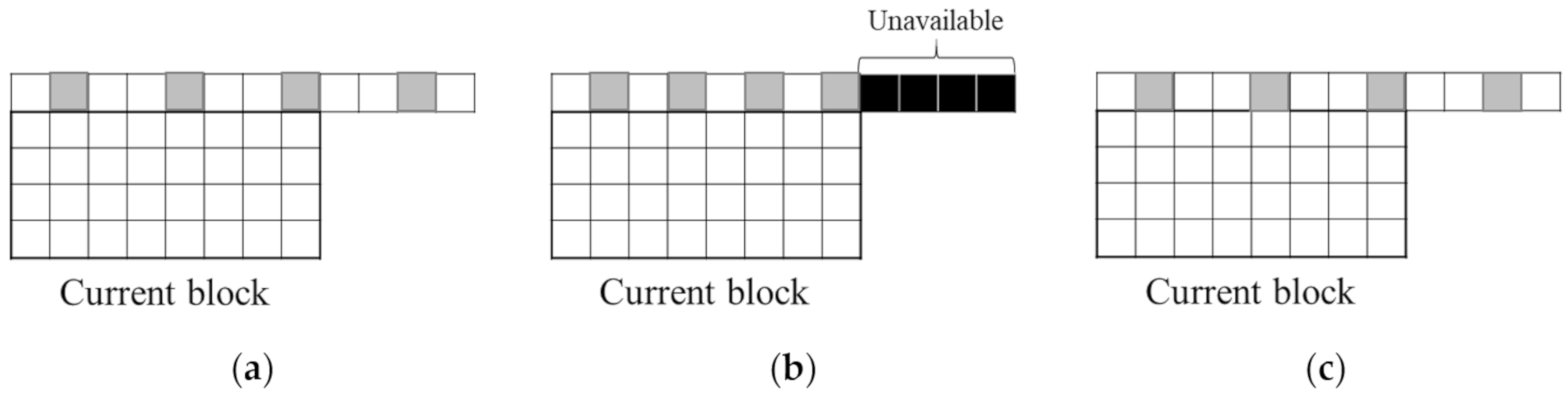
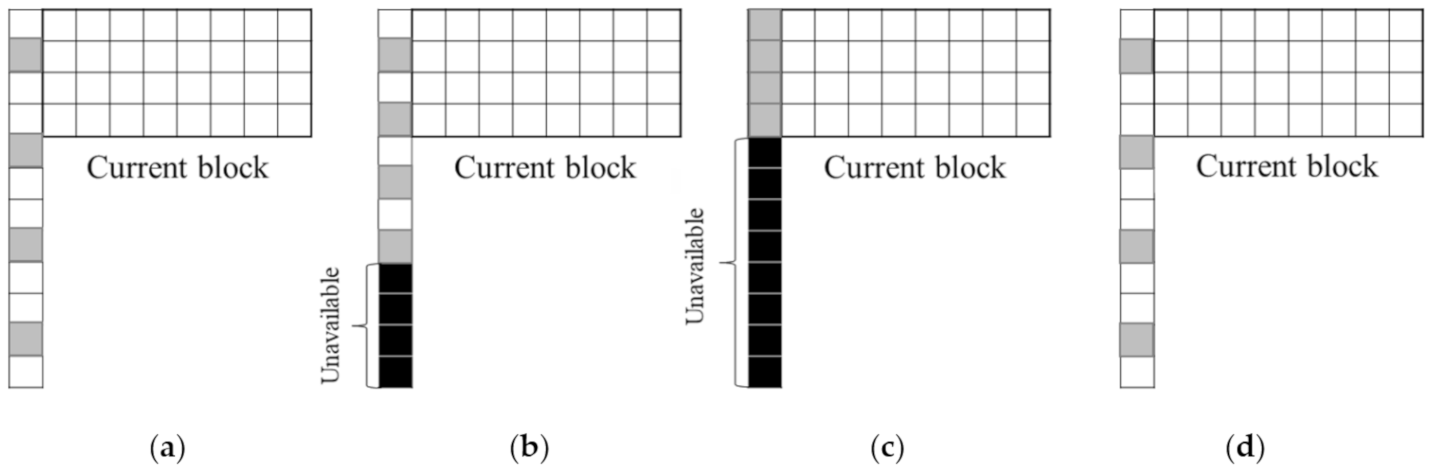
Compared to VTM-6.0, the subsampled neighboring sample positions of the proposed CCLM can be different because different sets of subsampled neighboring sample positions can be selected in VTM-6.0 according to the number of available neighboring samples. For a given 8 × 4 chroma block, Figure 8 and Figure 9 show the comparisons of the subsampled neighboring sample positions between VTM-6.0 and the proposed CCLM, for the T_CCLM and L_CCLM modes, respectively. In both figures, the square boxes indicate the sample positions, the gray boxes indicate the subsampled neighboring sample positions, and the black boxes represent the unavailable neighboring samples.

For the T_CCLM mode shown in Figure 8, based on the number of available top-right neighboring chroma samples, two different sets of subsampled neighboring sample positions can be selected in VTM-6.0, as shown in Figure 8a,b. On the other hand, in the proposed CCLM, only one set of fixed subsampled neighboring sample positions is derived, as shown in Figure 8c.

Furthermore, as can be seen from an example of the L_CCLM mode in Figure 9a–c, there are three different sets of subsampled neighboring sample positions in VTM-6.0, based on the number of available left-below neighboring chroma samples. However, one set of fixed subsampled neighboring sample positions is derived in the proposed CCLM, as shown in Figure 9d.

It is noted that the fixed subsampled neighboring sample positions are also applied to the subsampling of the corresponding neighboring luma samples.

3.4. Simplified Downsampling Filter for Luma Sample

As shown in Figure 3, Figure 4 and Figure 5, the luma sample downsampling process of the CCLM has many conditional branches according to sps_cclm_colocated_chroma_flag, the neighboring sample availabilities, the sample positions within the block, the subsampled sample positions for neighboring samples, and the CTU boundary condition. This results in various downsampling filter shapes for the luma sample. However, as all the neighboring luma samples are available using the neighboring sample generation process, the luma sample downsampling process can be significantly simplified. The conditions on the neighboring sample availabilities, the sample positions within the block, and the subsampled sample positions for neighboring samples are removed in the proposed CCLM, such that a simplified downsampling filter shape considering sps_cclm_colocated_chroma_flag and the CTU boundary condition is obtained.

Figure 10, Figure 11 and Figure 12 illustrate the simplified downsampling filter shapes for the collocated luma samples, the top neighboring luma samples, and the left neighboring luma samples, respectively. Figure 10 shows the flow chart of downsampling filter shape selection for the collocated luma samples in the proposed CCLM depending on the condition of sps_cclm_colocated_chroma_flag only, where one of two downsampling filter shapes is selected for downsampling of the collocated luma samples.

In Figure 11, the downsampling filter shapes of the top neighboring luma samples for the proposed CCLM are selected based on the sps_cclm_colocated_chroma_flag and the CTU boundary condition. It can be seen that up to three different downsampling filter shapes can be used for downsampling of the top neighboring luma samples.

Figure 12 shows the flow chart of downsampling filter shape selection for the left neighboring luma samples in the proposed CCLM, based on sps_cclm_colocated_chroma_flag only. In the figure, two different types of downsampling filter shapes can be chosen where the filter shapes are the same as in Figure 10.

3.5. Simplified Linear Model Parameter Derivation

The number of subsampled neighboring samples is dependent on the neighboring sample availabilities in VTM-6.0, so that additional operation and conditional branches are needed to derive the linear model parameters. The linear model parameters are derived by the equation of the straight line connecting two points, where the two points are calculated by the average value of two minimum values for each component, and the average value of two maximum values for each component. Accordingly, four sample values are required to derive the linear model parameters. However, the four sample values cannot be obtained in case the top or left boundary of the current block is the boundary of a picture, slice, or tile. For each component of the luma and the chroma, when the number of subsampled neighboring samples is equal to 2, the sample copy operation is performed to derive the four sample values using the two subsampled neighboring sample values.

On the other hand, in the proposed CCLM, four sample values are always available using the neighboring sample generation process; thus, the additional sample copy operation and the conditional branch to identify the number of sample values are removed, thereby simplifying the linear model parameter derivation process.

3.6. Comparative Analysis of the CCLM Design between VTM-6.0 and the Proposed CCLM

From an implementation point of view, a comparative analysis of the CCLM design, between VTM-6.0 and the proposed CCLM, is described as follows.

First, for analyzing the additional operations introduced by adding the neighboring sample generation process in the proposed CCLM,

Table 1. Comparison of the number of neighboring sample availability checks and the need for neighboring sample substitution process, between VTM-6.0 and the proposed CCLM, in the case of the LT_CCLM mode.

	Number of Neighboring Sample Availability Checks (in a 4 × 4 Block Unit)	Neighboring Sample Substitution Process
VTM-6.0	3 (top, left, and top-left sample positions)	Not needed
Proposed CCLM	5 (top, top-right, left, left-below, and top-left sample positions)	Needed

shows a comparison of the number of neighboring sample availability checks, and the need for neighboring sample substitution process between VTM-6.0 and the proposed CCLM, in the case of the LT_CCLM mode.

As listed in Table 1, the CCLM design in VTM-6.0 checks the neighboring sample availability of only three sample positions, including R(0, −1), R(−1, 0), and R(−1, −1), in a 4 × 4 block unit. By contrast, the proposed CCLM design checks the neighboring sample availability of five sample positions, including R(0, −1), R(2 × W − 1, −1), R(−1, 0), R(−1, 2 × H − 1), and R(−1, −1), in a 4 × 4 block unit, as well as requires the neighboring sample substitution process, as described in Section 3.1, because the neighboring sample generation process for general intra prediction is necessary. However, in hardware implementation, as the logics for the neighboring sample substitution process can be shared with those for general intra prediction, additional logics for the neighboring sample substitution process are not needed for the proposed CCLM.

Second, to compare the neighboring sample position derivation process between VTM-6.0 and the proposed CCLM, a comparison of the lengths of the top and left neighboring chroma samples between VTM-6.0 and the proposed CCLM is presented in

Table 2. Comparison of the lengths of the top and left neighboring chroma samples between VTM-6.0 and the proposed CCLM.

	LT_CCLM Mode		T_CCLM Mode	L_CCLM Mode
	Top Neighbor	Left Neighbor	Top Neighbor	Left Neighbor
VTM-6.0	0 or WC	0 or HC	WC ~ WC + min(NTR 1, HC)	HC ~ HC + min(NLB 1, WC)
Proposed CCLM	WC	HC	WC + min(WC, HC)	HC + min(HC, WC)

¹ Variable numbers depending on neighboring sample availabilities.

. For the LT_CCLM mode in VTM-6.0, the length of the top neighboring samples is either 0 or W_C, based on the availability of the top neighboring sample, and the length of the left neighboring samples is either 0 or H_C, based on the availability of the left neighboring sample.

Furthermore, the length of the top neighbor is in the range of W_C to W_C + min(N_TR, H_C) samples based on the available top-right neighboring chroma samples in the T_CCLM mode, and the length of the left neighbor is in the range of H_C to H_C + min(N_LB, W_C) samples based on the available left-below neighboring chroma samples in the L_CCLM mode. In VTM-6.0, the lengths of the top and left neighboring samples vary according to the neighboring sample availabilities. This results in a variable subsampled neighboring sample position derivation. On the other hand, in the proposed CCLM, the length of top neighbor in the LT_CCLM mode, the length of left neighbor in the LT_CCLM mode, the length of top neighbor in the T_CCLM mode, and the length of left neighbor in the L_CCLM mode are simply determined as W_C, H_C, W_C + min(W_C, H_C), and H_C + min(H_C, W_C), respectively. By using the proposed CCLM, the neighboring sample position derivation process is simplified, and fixed subsampled neighboring sample position derivation can be achieved. More specifically, for the T_CCLM mode, W_C/4 of the neighboring sample availability check is removed by the proposed CCLM, because the neighboring sample availability check can be done in a 4 × 4 block unit. Similarly, H_C/4 of the neighboring sample availability check for the L_CCLM mode is removed by the proposed CCLM.

Regarding the positions of subsampled neighboring samples,

Table 3. Comparison of the positions of subsampled neighboring samples between VTM-6.0 and the proposed CCLM in the case of a given 8 × 8 chroma block.

	LT_CCLM Mode	T_CCLM Mode	L_CCLM Mode
VTM−6.0	{RC(2, −1), RC(7, −1), RC(−1, 2), and RC(−1, 7)}, {RC(1, −1), RC(3, −1), RC(5, −1), and RC(7, −1)}, or {RC(−1, 1), RC(−1, 3), RC(−1, 5), and RC(−1, 7)}	{RC(2, −1), RC(6, −1), RC(10, −1), and RC(14, −1)}, {RC(1, −1), RC(4, −1), RC(7, −1), and RC(10, −1)}, or {RC(1, −1), RC(3, −1), RC(5, −1), and RC(7, −1)}	{RC(−1, 2), RC(−1, 6), RC(−1, 10), and RC(−1, 14)}, {RC(−1, 1), RC(−1, 4), RC(−1, 7), and RC(−1, 10)}, or {RC(−1, 1), RC(−1, 3), RC(−1, 5), and RC(−1, 7)}
Proposed CCLM	{RC(2, −1), RC(7, −1), RC(−1, 2), and RC(−1, 7)}	{RC(2, −1), RC(6, −1), RC(10, −1), and RC(14, −1)}	{RC(−1, 2), RC(−1, 6), RC(−1, 10), and RC(−1, 14)}

shows a comparison of the positions of the subsampled neighboring samples for deriving the linear model parameters between VTM-6.0 and the proposed CCLM, in the case of a given 8 × 8 chroma block.

As listed in Table 3, in case of the VTM-6.0, the positions of the subsampled neighboring samples can be different, according to the number of available neighboring samples. On the other hand, the subsampled neighboring sample positions can be fixed by the proposed CCLM. For a given 8 × 8 chroma block, in the proposed CCLM, up to three different sets of subsampled neighboring sample positions are reduced to one set of subsampled neighboring sample positions. Therefore, the operations for selecting different sets of subsampled neighboring sample positions are removed by the proposed CCLM.

Finally, an analysis of the number of downsampling filter shapes for the luma sample, according to the sample position, is provided as follows.

Table 4. Comparison of the number of downsampling filter shapes for the luma sample between VTM-6.0 and the proposed CCLM.

	Sample Position		sps_cclm_colocated_chroma_flag == 0	sps_cclm_colocated_chroma_flag == 1
VTM-6.0	Collocated luma block	i = 0, j = 0	2	4
		i > 0, j = 0	1	2
		i = 0, j > 0	2	2
		i > 0, j > 0	1	1
	Top neighboring luma sample	First subsampled sample position	4	4
		Non−first subsampled sample position	2	2
	Left neighboring luma sample		1	2
Proposed CCLM	Collocated luma block		1	1
	Top neighboring luma sample		2	2
	Left neighboring luma sample		1	1

shows a comparison of the number of downsampling filter shapes for the luma sample between VTM-6.0 and the proposed CCLM.

As listed in Table 4, for the downsampling of the collocated luma samples, when sps_cclm_colocated_chroma_flag is equal to 1, VTM-6.0 uses up to four different shapes of downsampling filter, whereas the proposed CCLM uses only one unified downsampling filter shape. Furthermore, up to four different shapes of downsampling filter for the top neighboring luma sample are used in VTM-6.0. However, in the proposed CCLM, up to two different shapes of downsampling filter are selected, according to only the CTU boundary condition. With regard to the conditional branch, 10 conditional branches for comparing various conditions, as shown in Figure 3, for the downsampling of collocated luma samples in VTM-6.0 are removed by the proposed CCLM. Similarly, nine conditional branches, as shown in Figure 4, for the downsampling of the top neighboring luma sample in VTM-6.0 are removed. Therefore, in the proposed CCLM, the conditions for selecting the different shapes of downsampling filter can be removed, thereby implementing the filtering operation by employing parallel processing.

4. Experimental Results

In this section, the experimental results of the proposed CCLM are provided to confirm whether the objective video quality is maintained by the proposed CCLM. The proposed CCLM was implemented on top of VTM-6.0. The experimental results of the proposed CCLM were compared to the VTM-6.0 anchor. The experiment was performed on a computer cluster consisting of Intel Xeon E5-2690 v2 (3.0 GHz) and 64 GB RAM, with a GCC 7.3.1 compiler using CentOS Linux, and was conducted following the JVET common test conditions, as specified in [31]. Two prediction structure configurations, which are “All Intra Main 10” (AI), “Random Access Main 10” (RA), were tested, and quantization parameters of 22, 27, 32, and 37 were used to obtain different rate points.

Table 5. Information on video sequences for each class.

Class	Sequence Name	Picture Size	Picture Count	Picture Rate	Bit Depth
A1	Tango2	3840 × 2160	294	60	10
	FoodMarket4	3840 × 2160	300	60	10
	Campfire	3840 × 2160	300	30	10
A2	CatRobot1	3840 × 2160	300	60	10
	DaylightRoad2	3840 × 2160	300	60	10
	ParkRunning3	3840 × 2160	300	50	10
B	MarketPlace	1920 × 1080	600	60	10
	RitualDance	1920 × 1080	600	60	10
	Cactus	1920 × 1080	500	50	8
	BasketballDrive	1920 × 1080	500	50	8
	BQTerrace	1920 × 1080	600	60	8
C	BasketballDrill	832 × 480	500	50	8
	BQMall	832 × 480	600	60	8
	PartyScene	832 × 480	500	50	8
	RaceHorses	832 × 480	300	30	8
D	BasketballPass	416 × 240	500	50	8
	BQSquare	416 × 240	600	60	8
	BlowingBubbles	416 × 240	500	50	8
	RaceHorses	416 × 240	300	30	8
E	FourPeople	1280 × 720	600	60	8
	Johnny	1280 × 720	600	60	8
	KristenAndSara	1280 × 720	600	60	8
F	BasketballDrillText	832 × 480	500	50	8
	ArenaOfValor	1920 × 1080	600	60	8
	SlideEditing	1280 × 720	300	30	8
	SlideShow	1280 × 720	500	20	8

lists the information on the classes of video sequences used in

Table 6. Experimental results of the proposed CCLM compared to VTM-6.0.

Class	Sequence	All Intra Main 10					Random Access Main 10
		Y	Cb	Cr	EncT	DecT	Y	Cb	Cr	EncT	DecT
A1	Tango2	0.03%	−0.05%	0.09%	99%	99%	0.04%	0.28%	0.05%	100%	100%
	FoodMarket4	0.01%	0.09%	0.12%	100%	99%	0.02%	0.16%	0.04%	100%	100%
	Campfire	−0.02%	0.40%	0.63%	100%	99%	0.02%	0.13%	0.68%	100%	99%
	Average	0.01%	0.14%	0.28%	100%	99%	0.03%	0.19%	0.26%	100%	99%
A2	CatRobot1	0.03%	0.01%	−0.05%	101%	99%	−0.01%	0.16%	0.07%	100%	99%
	DaylightRoad2	0.01%	0.22%	0.06%	101%	99%	0.07%	0.25%	0.20%	100%	100%
	ParkRunning3	−0.01%	0.08%	0.05%	99%	100%	0.02%	0.05%	0.09%	100%	100%
	Average	0.01%	0.10%	0.02%	100%	99%	0.03%	0.15%	0.12%	100%	100%
B	MarketPlace	0.01%	−0.05%	0.13%	99%	99%	−0.05%	0.30%	0.44%	100%	99%
	RitualDance	0.03%	−0.05%	−0.03%	100%	99%	0.00%	0.11%	−0.12%	100%	99%
	Cactus	0.01%	0.06%	0.02%	100%	100%	0.01%	0.22%	−0.03%	100%	100%
	BasketballDrive	0.01%	0.14%	−0.07%	101%	100%	0.00%	0.11%	0.13%	100%	100%
	BQTerrace	0.00%	−0.03%	0.05%	101%	100%	−0.05%	−0.03%	0.24%	100%	100%
	Average	0.01%	0.01%	0.02%	100%	99%	−0.02%	0.14%	0.13%	100%	100%
C	BasketballDrill	0.01%	0.10%	−0.17%	101%	100%	0.02%	0.36%	0.01%	100%	99%
	BQMall	0.03%	−0.07%	−0.01%	100%	99%	0.02%	−0.21%	0.08%	100%	99%
	PartyScene	0.00%	−0.02%	−0.02%	100%	100%	0.01%	−0.06%	0.02%	100%	99%
	RaceHorses	0.02%	−0.18%	0.06%	100%	100%	0.00%	0.05%	0.21%	100%	99%
	Average	0.02%	−0.04%	−0.03%	100%	100%	0.01%	0.04%	0.08%	100%	99%
E	FourPeople	0.01%	−0.01%	−0.04%	99%	99%	—	—	—	—	—
	Johnny	−0.01%	−0.19%	0.40%	100%	99%	—	—	—	—	—
	KristenAndSara	−0.01%	0.03%	−0.15%	100%	100%	—	—	—	—	—
	Average	0.00%	−0.05%	0.07%	100%	99%	—	—	—	—	—
	Overall	0.01%	0.03%	0.06%	100%	99%	0.01%	0.13%	0.14%	100%	99%
D	BasketballPass	0.03%	0.27%	−0.09%	100%	99%	−0.03%	0.26%	0.07%	100%	99%
	BQSquare	0.00%	−0.11%	−0.24%	100%	100%	−0.04%	−0.13%	−0.20%	101%	99%
	BlowingBubbles	0.02%	−0.06%	−0.34%	100%	99%	−0.10%	−0.49%	−0.13%	100%	99%
	RaceHorses	−0.06%	−0.18%	0.07%	101%	99%	−0.07%	−0.06%	0.31%	99%	99%
	Average	0.00%	−0.02%	−0.15%	100%	99%	−0.06%	−0.10%	0.01%	100%	99%
F	BasketballDrillText	0.00%	0.01%	0.06%	100%	100%	0.01%	0.19%	0.03%	100%	99%
	ArenaOfValor	0.02%	0.13%	0.11%	100%	100%	0.03%	0.00%	−0.01%	100%	99%
	SlideEditing	0.04%	0.05%	0.16%	100%	99%	−0.06%	0.11%	0.10%	100%	98%
	SlideShow	0.09%	−0.04%	0.22%	100%	99%	−0.01%	−0.07%	0.23%	100%	99%
	Average	0.04%	0.04%	0.14%	100%	99%	−0.01%	0.06%	0.09%	100%	99%

.

Table 6 summarizes the experimental results of the proposed CCLM compared to those of the anchor. In Table 6, the runtime reduction was calculated based on the ratio of the test to the anchor. “EncT” and “DecT” refer to the total encoding time ratio and the total decoding time ratio to the anchor at the encoder and the decoder, respectively. For example, if “DecT” is less than 100%, the test reduced the total decoding time compared to those of the anchor. Meanwhile, the BD-rate indicates the bit rate reduction ratio over the anchor achieved by the test when maintaining an equivalent peak signal-to-noise ratio (PSNR). For example, a negative BD-rate value means that the coding efficiency was improved. In the results, the BD-rates for the Y, Cb, and Cr components were calculated; “Overall” BD-rate means the average BD-rate for each component over Classes A1, A2, B, C, and E excluding Classes D and F. It should be noted that the experiments of Class E sequences under RA configuration were not conducted according to the JVET common test conditions. As listed in Table 6, for the AI configuration, the overall BD-rates of 0.01%, 0.03%, and 0.06% were observed for the Y, Cb, and Cr components, respectively. Additionally, for the RA configuration, the overall BD-rates of 0.01%, 0.13%, and 0.14% were observed for the Y, Cb, and Cr components, respectively, as presented in Table 6. In the proposed CCLM, as the unavailable neighboring samples are replaced with the adjacent available samples, the sample positions with the replicated sample values can be selected in the neighboring sample position derivation process. Moreover, in the luma sample downsampling process, the replicated sample values are also used as input to the downsampling filtering. Therefore, these led to minor coding losses, because inaccurate linear model parameters were derived, when compared to VTM-6.0.

Comparing the BD-rate results for each component, the overall BD-rates of the Y component for all classes were in the range of 0.00% to 0.04%, and −0.06% to 0.03%, for the AI and RA configurations, respectively. For the Cb component, the overall BD-rates for all classes were in the range of −0.05% to 0.14%, and −0.10% to 0.19%, for the AI and RA configurations, respectively. Furthermore, the overall BD-rates of the Cr component for all classes were in the range of −0.15% to 0.28%, and 0.01% to 0.26%, for the AI and RA configurations, respectively. According to these results, it can be seen that the BD-rate variations in the chroma components were larger than those of the luma component under the same PSNR. The BD-rate variation in the luma component was mainly caused by the use of a simplified downsampling filter for the luma sample. The simplified and fixed subsampled neighboring sample position derivation led to BD-rate variations in the chroma components. However, it should be noted that the BD-rate impacts of each component in the proposed CCLM are negligible. Furthermore, especially for the Campfire sequence, BD-rates of the Cr component showed the largest coding loss in both the AI and RA configurations. As the Campfire sequence has a large sample value variation of the chroma component, between a bright fire in the foreground and a dark black background, the unavailable samples can be substituted by an inaccurate adjacent sample value, which may have a large difference in sample value from the unavailable sample. It seems that the coding loss is caused by the fact that the neighboring sample substitution process in VVC does not consider the sample value in its process. As can be seen from Table 6, the overall ratios of total encoding time for the AI and RA configurations were 100% and 100%, respectively. Furthermore, the overall ratios of the total decoding time for the AI and RA configurations were 99% and 99%, respectively, as shown in Table 6. The proposed CCLM demonstrated a decrease in decoding time since it simplifies the neighboring sample position derivation process, the luma sample downsampling process, and the linear model parameter derivation process, despite the addition of the neighboring sample generation process to the CCLM mode. In addition, the total decoding time reduction was observed, rather than the total encoding time reduction, because the proportion of time required to perform the CCLM mode in total decoding time is greater than that required to perform the CCLM mode in total encoding time, due to the mode decision in the encoder. It can be noted that the proposed CCLM reduced not only the implementation complexity, but also the runtime complexity, as shown by the reduction in the total decoding time.

From the experimental results, it can be noted that the proposed CCLM can be efficiently implemented by employing parallel processing under negligible BD-rate impacts compared to VTM-6.0.

5. Conclusions

The proposed CCLM removes many conditional branches for checking the neighboring sample availability, and simplifies downsampling filter shapes for the luma sample. The main idea of the proposed CCLM is that the neighboring sample generation process specified in VVC is added to the CCLM as the first process, so that unavailable neighboring samples can be replaced with the adjacent available samples. Owing to the reduction of the conditional branches and the simplification of luma downsampling filters, the proposed CCLM can be efficiently implemented by employing parallel processing in both hardware and software implementations. It is noted that additional logics for the neighboring sample substitution process are not needed for the proposed CCLM, because the logics can be shared with those for general intra prediction in hardware implementation.

As for future work, we plan to improve the fixed neighboring sample position derivation process based on a game theory-based approach, such as proposed in [32].