1. Introduction
In the next generation wireless communication systems, massive multiple-input-multiple-output (MIMO), in which a large number of antennas are utilized, is considered one of the key technologies that will be used to increase system capacity [
1]. In massive MIMO, beams can be generated to transmit or receive signals in a desired direction, which enables a much larger gain compared with single antenna systems. However, if a beam is generated in a wrong direction (i.e., a null point), the signal gain is severely deteriorated and could possibly be even lower than that obtained using a single antenna. Consequently, generating a proper beam is one of the most important research topics to be considered in massive MIMO system [
2,
3].
The optimal beamforming vector can be found analytically based on complete channel state information [
4]. However, when the number of antennas is large, it is impossible to obtain complete channel state information due to the very large signaling overhead involved. Even in channel reciprocal systems where uplink training can be used to obtain channel information with a small overhead, the number of required pilot sequences for uplink training is greater than the total number of antennas at the user equipment (UE), such that the signaling overhead is likely to be huge [
2]. Accordingly, researchers have tended to focus on beamforming schemes that can operate with limited channel feedback or with an imperfect channel state information.
The use of a limited set of beamforming vectors has been considered as a practical alternative to continuous beam weight control [
3] in order to overcome the signaling overhead problem. The transceiver can then switch beams among a predefined beam set. In switched beamforming, the base station (BS) performs an exhaustive search of a set of predefined beam vectors to find the optimal beam vector, that is, evaluating the achievable capacity for all possible beam vectors and choosing the one with the maximum capacity. For example, the IEEE 802.11ad standard specifies a procedure for finding the proper beam [
5], which is divided into two stages; the first stage is the sector level sweep (SLS) and the second is the beam refinement process (BRP). This type of beam search procedure can take quite a long time and possibly require a large amount of resources, therefore, efficient beam search procedure, that is, beam selection algorithms, should be investigated.
In recent years, the use of deep learning has yielded remarkable improvements in cognitive tasks such as image processing, speech recognition and natural language processing. In deep learning, multilayer perceptrons (MLPs) are connected from input layer to output layer by mimicking the human brain. Such a structure enables complicated nonlinear representations to be learned autonomously by using a large number of training data. Interestingly, the architecture of a deep neural network (DNN) leads to outstanding performance not only as a classifier but also in deep reinforcement learning, where an agent tries to find an appropriate course of action that maximizes the cumulative reward. The authors of Reference [
6] proposed the application of DNN in reinforcement learning, showing that with the aid of DNN, the reinforcement learning algorithm performs as well as human level, or even better in playing Atari games. In addition, there has been some attempts to apply deep learning to wireless communications systems. In particular, the beam search (or else called beam selection) problem in massive MIMO systems can be tackled with deep learning. In Reference [
7], which is improved from Reference [
8], two stage beamforming scheme is replaced with two separate neural network blocks, where each network works as antenna selection and RF chain selection respectively. Given that the hybrid beamforming MIMO systems were considered, these schemes cannot be directly applied to our system model in which massive antenna with a single RF was considered. Also, beam selection algorithm based on deep learning with the aid of scene data was proposed in Reference [
9]. They used additional information of scene data which is composed of the geographical data, for example, position and length of cars, to increase accuracy of beam selection such that the scheme is only feasible if the scene data is available, whereas only the instantaneous channel data is used in our proposed scheme.
Herein, we propose a deep reinforcement learning architecture, thereby producing a novel beamforming vector selection scheme in a massive MIMO system which can determine the proper beamforming vector using a single pilot signal. The main contributions of this paper can be summarized as follows.
We adopt deep reinforcement learning (deep Q-learning) in order to solve the beamforming vector determination problem in a massive MIMO system. To our best knowledge, our work is the first attempt to merge deep reinforcement learning with massive MIMO beam scanning.
We show that the Deep Scanning proposed here can significantly reduce the time and complexity involved in finding the optimal serving beam for UE through simulations. As opposed to conventional schemes, the complexity of our scheme is not proportional to the number of beamforming vectors or the number of antennas, which makes our proposed scheme appropriate for practical massive MIMO systems.
The remainder of this paper is organized as follows. In
Section 2, we describe the system model considered in this paper, and in
Section 3, we propose deep reinforcement learning architecture for massive MIMO based beamforming. The performance of the proposed scheme is then evaluated in
Section 4, followed by our conclusions in
Section 5.
2. System Model
We assume that a BS is equipped with antennas in a planar array shape whose size is , and a UE has antennas, where . We consider uplink transmission where the BS utilizes receive beamforming in order to receive signal from a UE. Although we consider uplink transmission, our proposed scheme can also be applied to downlink transmission as well when the channel reciprocity between the uplink and downlink channels exists.
In our system model, the received signal at the BS without receive beamforming can be expressed as follows.
Here, denotes the signal received from the UE at the BS without receive beamforming, is the channel coefficient matrix between the BS and UE, and denotes the pilot signal of UE. Also, denotes the noise which follows a normal distribution with zero mean and variance . In addition, refers to a complex number set.
When receive beamforming is applied, the received signal,
, and resulting capacity for UE,
C, can be denoted as follows.
where
W is the bandwidth,
is the transmit power,
is the receive beamforming vector, and † denotes complex conjugate.
Herein, we consider a Discrete Fourier Transform (DFT) based beamforming [
10], which is a phased array beamforming method, cf.
Figure 1. To be more specific, in order to concentrate the antenna gain in a specific direction
and
, which are the azimuth and elevation of the direction, respectively, the weight of the antennas must be set as follows.
In (3),
is the weight of antenna whose indexes are
and
. Moreover,
and
denote the antenna coordinate on the y-axis and z-axis, respectively, where the antennas are distributed in the Y-Z plane, cf.
Figure 1. The receive beamforming vector then becomes
.
In our system model,
B predefined beamforming vectors are considered, that is, the possible values of
and
are fixed, such that our goal is to find the beamforming vector
that maximizes the channel capacity, among
B predefined beam vectors whose set is denoted as
. It should be noted that the determination of the appropriate beamforming vector is non-trivial because the channel between the BS and the UE is not generally Line-of-Sight (LoS), and the beam pointing to the UE may not provide the maximal channel capacity for that UE. It is also worth noting that the proposed beam searching scheme can also contribute to a hybrid beamforming system where the first stage beamforming utilizes DFT beamforming for a UE [
3].
3. Proposed Scheme
In this paper, we propose Deep Scanning in which the double deep Q-learning [
11,
12] is applied to beamforming vector selection. Deep reinforcement learning has been taken into account instead of supervised learning, in order to reduce the overhead entailed in collecting the train dataset and to better adapt to the wireless environment. To be more specific, in supervised learning, a large set of labeled data is required for training such that a huge overhead is associated with obtaining this labeled dataset. Moreover, unlike supervised learning, the reinforcement learning can adjust its operation in an adaptive manner due to the use of the discount parameters, such that we have taken into account reinforcement learning in our proposed scheme. More details are explained in the later part of this section.
To this end, the observing state (), action () and instant reward () for time t, which constitutes the Q-learning framework, are defined as follows.
In our Q-learning framework,
is the received signal at the BS,
is the receive beamforming vector and
is the channel capacity, which can be achieved by action
at state
. It is worth noting that the observing state is continuous such that the size of state space is infinite. The formulated state and action satisfy the Markov Decision Process (MDP) property such that the next state depends only on the present state and action. As a consequence, the use of Bellman equation-based Q-learning can be validated where the Q-value, which refers to the expected reward in consideration of discounted future rewards of an action
a given a state
s, is found in an iterative manner. Mathematically, the optimal Q-value,
, can be expressed by the Bellman equation as follows.
where
is the next state which is determined by the current state
s and the current action
a. When
is given, the optimal action for state
s can be determined as
. Moreover,
is the discount parameter that models a decaying effect of the future rewards. This Q-function definition allows the retraining of RL based scheme to adapt to a new environment much faster than the supervised learning based scheme. It is mainly due to the fact that unlike the supervised learning which takes into account each training data equally in the update of parameters (weights and biases) of neural network, in the RL based scheme, the recent training data has larger impact on the update of the parameters of neural network compared with the old training data. Specifically, as can be seen from the loss function used in our proposed scheme which is shown in (5) on the next page, we have taken into account the discount factor,
, where
, such that old information will have minor effect on the update of the parameters of neural network. Given that the training data can be continuously collected during the execution of our proposed scheme due to the nature of RL, our proposed scheme can adjust its operation according to varying propagation environment.
However, in our system model, it is difficult to derive the optimal Q-value using conventional iterative methods because the size of state space is infinite. To solve this problem, we apply deep Q-learning which works well for an infinite state space [
6]. Specifically, in deep Q-learning, Q-values are found using a convolutional neural network (CNN) known as a Q-network, which is able to handle continuous state space, rather than building a Q-table that contains Q-values for all possible combinations of states and actions. Specifically, the Q-network operates as a Q-value approximator in which an action is chosen to maximize the total expected rewards. In Deep Scanning, the received signal
is fed into the trained CNN structure, which gives the Q-values for all beamforming vectors in
(i.e., actions). Then, the beamforming vector with the greatest Q-value can be chosen.
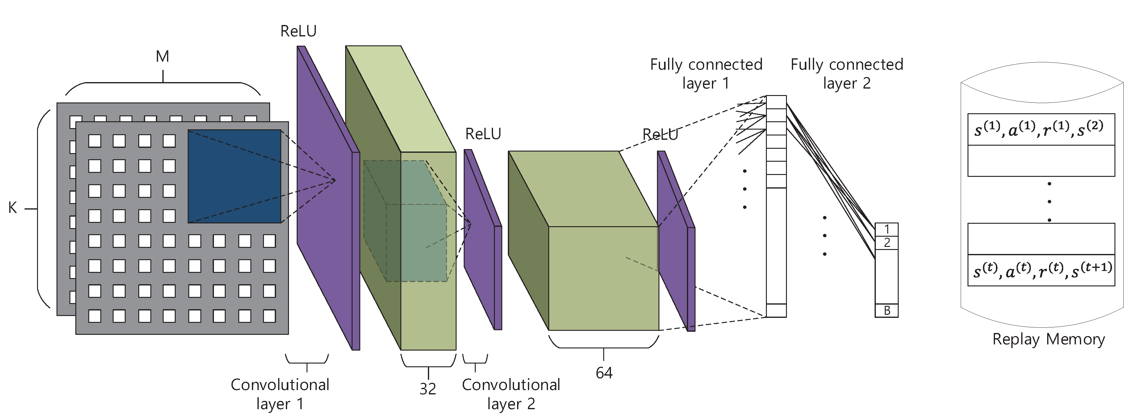
The Q-network for Deep Scanning is composed of two convolutional layers and two fully connected layers as depicted in
Figure 2. The input of the Q-network is two real valued matrices whose shapes are
. The elements of these matrices correspond to the magnitude and phase of the received signal at each antenna of the BS. These two matrices are fed into two convolutional layers with stride 2 where each convolutional layer is followed by a rectifier linear unit(ReLU) layer. Herein, the convolutional layer performs 2D spatial convolution and the ReLU layer performs
such that the negative inputs are nullified. The sizes of spatial filter in the first and second convolutional layer are set to
and
, respectively, and the depth of the layer is set to 32 and 64, respectively. These convolutional layers are used to extract spatial features from the input layer of the received data. After the spatial features have been extracted by the convolutional layer, the ReLU layers give non-linearity to the deep Q-network [
13]. The output of the convolutional layers is fed into two fully connected layers, each followed by a ReLU layer allowing the results of convolutional layers to be properly combined such that the Q-value of each beamforming vector is calculated. In addition, the Q-network also has a replay memory, which stores the current state (received signals), selected action (beamforming vector), current reward (channel capacity achieved by selected beamforming vector), and the next state, [
], for each of input data, and is used during the training.
In our proposed deep Q-learning, the Q-network is trained to minimize the following loss function, which is the difference between the current Q-value and the optimal Q-value approximated by an older network [
11,
12].
In the loss function,
is the Q-value approximated by the current Q-network where the weights of the CNN are
and
is the Q-value approximated by a C-step older Q-network whose weights are
. Note that the Q-network becomes myopic, that is, only the current reward is taken into account, when
. Since we use an old (
) and a new (
) Q-network simultaneously during training, it becomes double deep Q-learning, which has been shown to be robust to divergence and oscillation compared with single deep Q-learning [
12].
The training of the Deep Scanning is divided into two stages, namely observe and explore. In the observe stage, current state, selected action, current reward, next state which are resulted from random beamforming vector selection are stacked into the replay memory without adjustment of the weights in the CNN. Second, in the explore stage, the Q-network is trained using an -greedy algorithm where for each state, the beamforming vector is randomly chosen with a probability of (exploration) and the beamforming vector with the highest Q-value is chosen with a probability of (exploitation). Specifically, during training, the value of decreases from 1.0 to 0.0 so that the Q-network can be trained for various different situations. In this stage, the stochastic gradient descent (SGD) method is used in which the 100 training samples are randomly chosen for a batch from the replay memory. Finally, after finishing the training, the value of is set to 0 and the trained CNN is used for the beamforming vector selection (inference stage). It is worth noting that only the state s is needed, which can be acquired from a single pilot signal that is, full channel information is not needed.
4. Performance Evaluation and Discussion
In this section, we present simulation results that show the performance of Deep Scanning, that is, the probability of selecting the optimal beamforming vector, the channel capacity, and the searching complexity. In order to consider a practical and generic wireless environment, we generate a geometric channel based on the WINNER II channel model [
14] such that the multipath channel with 3-dimensional field pattern is considered in the performance evaluation. The transmit power and noise power are assumed to be 30 dBm and −174 dBm/Hz, respectively, and the center frequency is 2.4 GHz with a working bandwidth of 10 MHz. A BS has quasi-omni coverage with 10 sector beams, that is,
= 10. The UE is randomly placed within the coverage of the BS. We assume the BS has a 12 × 12 planar array antenna that is,
, and a UE has 4 antennas, that is,
.
Also, 3000 epochs are used to train DNN where each epoch is composed of 100 samples. Of 3000 epochs, first 500 epochs are used for exploration and rest 2500 epochs are used for exploitation with linearly decreasing from 1 to 0, so that there is no random selection at the end of training. For the testing, we randomly generated 5000 channel realizations. The simulation duration depends on the performance of computers, however, it would be helpful to provide our simulation duration, that is, 16 h, to give a glimpse to the readers.
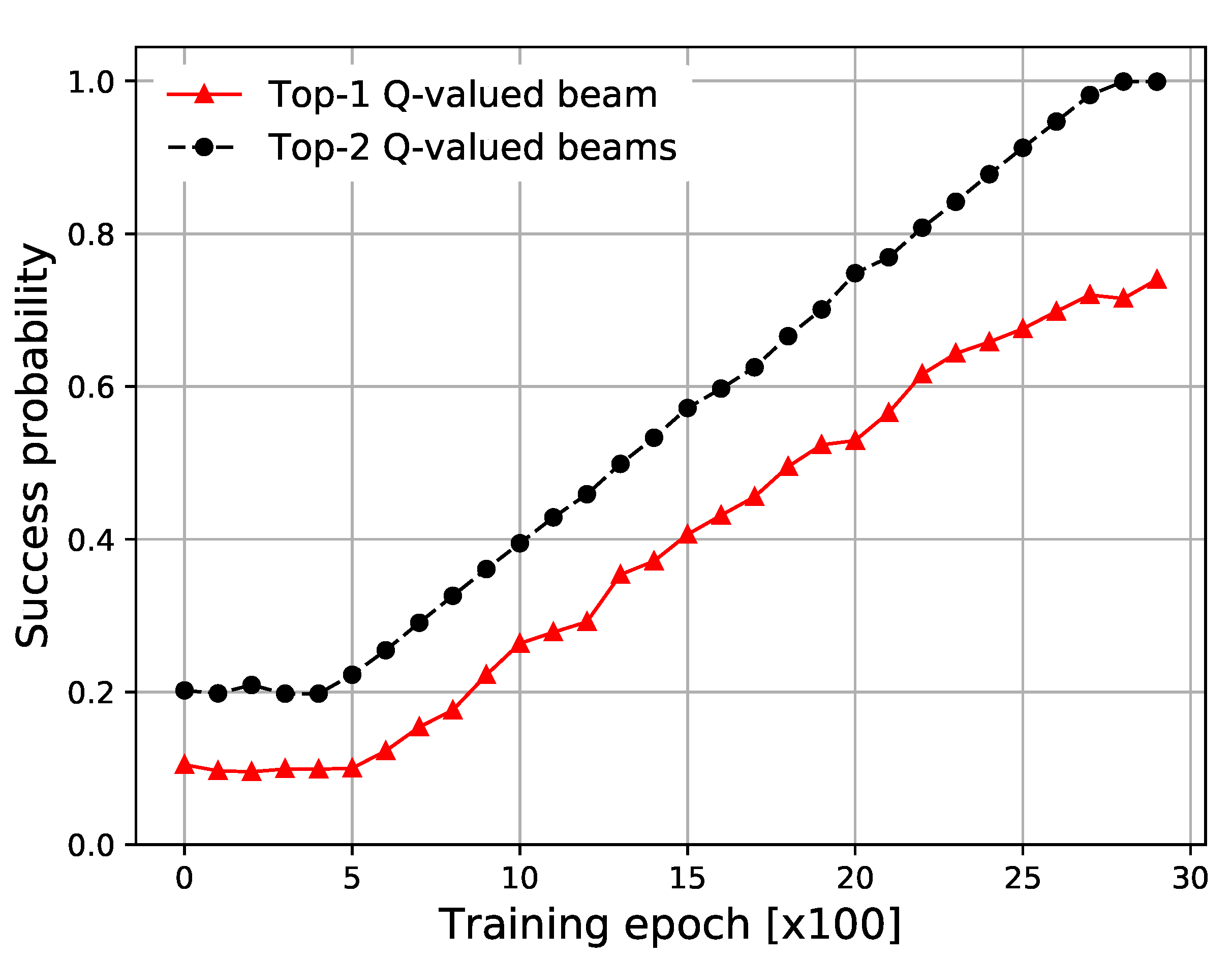
In
Figure 3, we show the success probability, which is the probability that the optimal beamforming vector is found during the proposed Deep Scanning. In the simulation results, ‘Top-1’ is the success probability that the optimal beamforming vector is matched with the highest Q-valued beamforming vector from the Q-network and ‘Top-2’ is the success probability that the optimal beamforming vector is correctly matched with the highest or second highest Q-valued beamforming vector from the Q-network. Top-1 and Top-2 can be seen to reach values of 0.7 and 1.0, respectively.
In addition, we can see that the success probability starts at around 0.1 for the observation stage because during this stage, the serving beamforming vector is randomly chosen out of 10 beamforming vectors.
In
Figure 4, we compare the channel capacity of our proposed scheme with that can be achieved using an exhaustive beam search, denoted by optimal capacity and also with a Least Square (LS) channel estimation scheme, in which the squared value of difference between the original and estimated signal is minimized for given pilot sequence [
2]. In the simulation results, ‘Top-1 beam’ is the capacity when the beamforming vector with highest Q-value is used and ‘Top-2 beam’ is the capacity when the highest and second highest Q-valued beamforming vectors are alternately used. As the number of used beamforming vectors increases, the channel capacity also increases, because the directional gain of the antenna increases. The capacities of both ‘Top-1 beam’ and ‘Top-2 beams’ are close to the optimal values where ‘Top-2 beams’ shows a higher capacity than ‘Top-1 beam’. The gap between the optimal capacity and the capacity of the proposed scheme is due to the huge difference between the capacity for the optimal beamforming vector and that for a non-optimal beamforming vector.
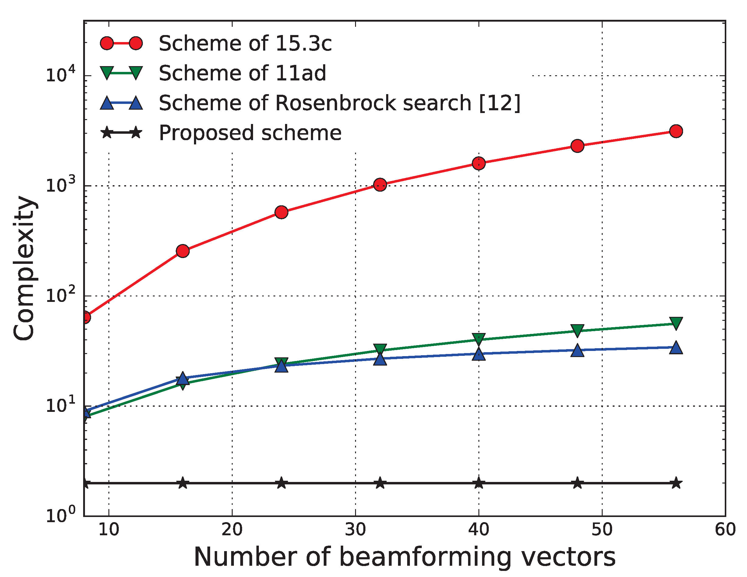
In
Figure 5, we compare the complexity, in terms of the number of trials to be attempted to select the best beam, of our proposed scheme with that of conventional beam search algorithms. It should be noted that the LS scheme requires a single pilot transmission such that the beam searching complexity of the LS scheme is the same as that of the proposed scheme, and hence it is not shown in
Figure 5. Our proposed beam searching procedure requires training using a number of samples, but, once it is trained, the optimal beamforming vector can be found with negligible computational complexity. Therefore, the beam searching complexity of our scheme depends neither on the number of antennas nor on the number of predefined beamforming vectors, as can be seen from the simulation results, unlike in conventional schemes [
5,
15,
16], where the complexity increases with the number of beamforming vectors. Although it is not shown in the figure, the exhaustive search can be used to find the optimal beam. When the number of possible beams is small, for example,
, the proposed scheme which is based on reinforcement learning (RL), has only minor advantage over the exhaustive search, however, when the number of possible beams is large, the complexity of our proposed scheme will be significantly smaller than that of the exhaustive search. Moreover, when the adjustment of beam is performed in a continuous manner, that is, the number of possible beams is infinite, it is impossible to utilize the exhaustive search and the benefit of our proposed scheme is evident. In summary, for the massive multiple-input-multiple-output (MIMO) system which can possibly have large number of possible beams and even infinite number of possible beams due to continuous beam formulation, our proposed scheme based on RL will be beneficial than the exhaustive search scheme in terms of computational complexity. It should be noted that the tradeoff between the success probability of choosing the optimal beam and the searching complexity is inevitable, therefore, the major goal of our beam selection scheme is to achieve the larger capacity while keeping the searching complexity low.


