FPGA-Based Optical Surface Inspection of Wind Turbine Rotor Blades Using Quantized Neural Networks

Abstract

Quantization of the weights and activations of a neural network is a way to drastically reduce necessary memory accesses and to replace arithmetic operations with bit-wise operations. This is especially beneficial for the implementation on field-programmable gate array (FPGA) technology that is particularly suitable for embedded systems due to its low power consumption. In this paper, we propose an in-situ defect detection system utilizing a quantized neural network implemented on an FPGA for an automated surface inspection of wind turbine rotor blades using unpiloted aerial vehicles (UAVs). Contrary to the usual approach of offline defect detection, our approach prevents major downtimes and hence expenses. To our best knowledge, our work is among the first to transfer neural networks with weight and activation quantization into a tangible application. We achieve promising results with our network trained on our dataset consisting of 8024 good and defected rotor blade patches. Compared to a conventional network using floating-point arithmetic, we show that the classification accuracy we achieve is only slightly reduced by approximately $0.6$%. With this work, we present a basic system for in-situ defect detection with versatile usability.

1. Introduction

Since 1992, the cumulative energy output, as well as the number of wind turbines, have continuously increased By 2017, wind energy plants were responsible for approximately 49% of renewable energy in Germany [1]. Further gains in efficiency and energy yield are achieved by constructing increasingly large plants. This, in turn, increases the amount of environmental stress these plants are exposed to, which entails regular inspection, maintenance and repair by the operators. These cause considerable downtimes and expenses due to the manual inspection process. The conventional approach consists of visual inspection by trained technicians. There also exists a variety of support systems, e.g., man-carrying platforms, rope systems or cranes. However, manual inspection is still costly and the automation of the inspection process has hence become a long-standing goal of researchers and operators [2]. One such approach is the use of unpiloted aerial vehicles (UAV), as they provide a fast and flexible platform for positioning sensors close to different areas of the wind turbine. Multiple such approaches have hence been proposed and implemented [3,4,5]. A key component for further automating such systems is automatic real-time defect detection. This would not only speed up the inspection process by decreasing the need for human intervention but also open new possibilities for implementing more dynamic measurement routines. Particularly, if real-time or close-to-real-time performance is achieved, the UAV could, e.g., automatically adapt to improper lighting conditions or ambiguous defect detection results by changing the measurement angle or taking multiple images from different perspectives.

To augment existing UAV-based approaches for wind turbine inspection, the defect detection algorithm must be able to achieve high defect detection with a very low false alarm rate. Furthermore, it has to be possible to run it in real-time on a low-weight and low-power hardware system. A promising candidate for the development of such algorithms are convolutional neural networks (CNN) as they have consistently found success in a variety of image processing tasks ranging from image classification [6] to image segmentation and have hence also been successfully applied to surface inspection tasks [7,8,9]. However, CNNs require suitable hardware to achieve real-time performance. A common solution is to use GPU-based systems, e.g., NVIDIA’s Jetson boards, but recent advantages in applying deep learning methods with limited numerical precision [10] and particularly the introduction of binarized neural networks [11,12] have opened new possibilities to utilize alternative hardware systems, such as field-programmable gate arrays (FPGA), to implement CNNs. While GPU-based embedded systems are optimized in terms of achieving high performance at low power consumption, FPGA-based systems hold the potential to further reduce power consumption by at least one order of magnitude. Even for basic tasks, the power consumption of the commonly used Nvidia GeForce GTX 1080 TI graphic card alone is higher than that of the complete FPGA platform [13].

We introduce a system for real-time defect detection of rotor blades utilizing a drone. Our proposed approach deals with the application of an FPGA-based system for the classification of damaged and undamaged rotor blades using binarized convolutional neural networks (BCNN). An Arty Z7-20 development platform containing a Xilinx XC7Z020-1CLG400C FPGA and a Dual ARM Cortex A9 microprocessor is used as the basic system. By using that combination, different tasks can be distributed to one of the components to benefit from their particular special abilities. The proposed subsystem represents the core element of our project, which is highly important for the real-time capability.

Multiple approaches for utilizing UAVs for inspecting wind turbines have been proposed and implemented. For example, the authors of [5] discussed the factors that influence measurement quality when inspecting different structures with UAVs. Stokkeland et al. presented a routine based on the Hough transform for detecting wind turbine towers, hub and blades as well as the Kalman filter for tracking [4]. They also showed that their method can be executed in real-time on a single board computer carried with the UAV. The authors of [3] used photogrammetry software to reconstruct a 3D profile of rotor blades based on images captured with a UAV, which also contains defects, discontinuities, and markings and can hence be used for surface inspection. As for the automatic surface inspection of wind turbine rotor blades, Wang et al. proposed a method based on Haar-like features and classification via an extended cascading classifier with LogitBoost, decision trees and support vector machines to detect surface cracks on wind turbine rotor blades [14].

Over the last years, convolutional neural networks became the most commonly used approach for image analyses such as classification, object detection and image segmentation, for both two- and three-dimensional data [15,16,17,18,19,20]. Denhof et al. recently conducted an extensive investigation using different pre-trained convolutional neural network (CNN) model architectures for the detection of surface defects on wind turbine rotor blades [21]. Shihavuddin et al. also proposed a complete defect detection pipeline based on CNNs [22]. As for the implementation of CNN-based defect detection in an on-board solution, i.e., directly attached to the UAV, we could not find any previous work. However, a growing number of studies investigates the implementation of CNNs on FPGAs. A key idea behind this is the introduction of so-called binarized convolutional neural networks (BCNN) [12,23]. Using that, the weights and activations of the network’s neurons are quantized to a defined amount of bits and, in the extreme case, binarized, i.e., they only know two different states, and hence are representable by one bit. Thus, most arithmetic operations during the forward pass, i.e., when feeding the network with data to be classified, are replaced by bit-wise operations, which greatly reduces memory consumption and the number of memory accesses. Hence, the calculation can be done more power-efficiently [12]. Several studies confirm the efficiency of BCNNs on image classification tasks [11,12,23]. All of them use common benchmarks like MNIST or CIFAR. Zhou et al. generalized the idea of training low bit-width convolutional neural networks by introducing DoReFa-net [24], where they present methods for the quantization of weights, activations and gradients and show the efficiency of their method on the Street View House Numbers (SVHN) and the ImageNet datasets [25]. Sanaullah et al. presented an FPGA-based implementation of a multilayer-perceptron for real-time data analysis for medical diagnosis [26], showing the applicability of binarized neural networks in combination with FPGAs in a real-world application. They highlighted the advantages of the possibility of direct interfacing peripheral hardware such as sensors, actuators or memory blocks and achieve promising results with a high increase of processing speed.

To our knowledge, our work is among the first to translate the used quantized neural networks into a tangible image processing application. Through our work, we prove the suitability of low-power embedded systems for surface inspection tasks.

2. Materials and Methods

In this section, we present our proposed methods. First, we explain the structural properties of the binarized neural network. Afterwards, we elaborate on the training and the transformation into the FPGA hardware.

2.1. Binarized Convolutional Neural Networks

BCNNs use binary weights and activation functions instead of real numbers such as their standard floating-point counterparts. Floating-point arithmetic, especially multiplications that are used in deep learning, e.g., during gradient calculation and parameter updating, is highly computation-intensive, which complicates an implementation on hardware such as FPGAs. Convolutional layers are more affected by that than fully-connected layers, which are in comparison more memory-consuming [27]. 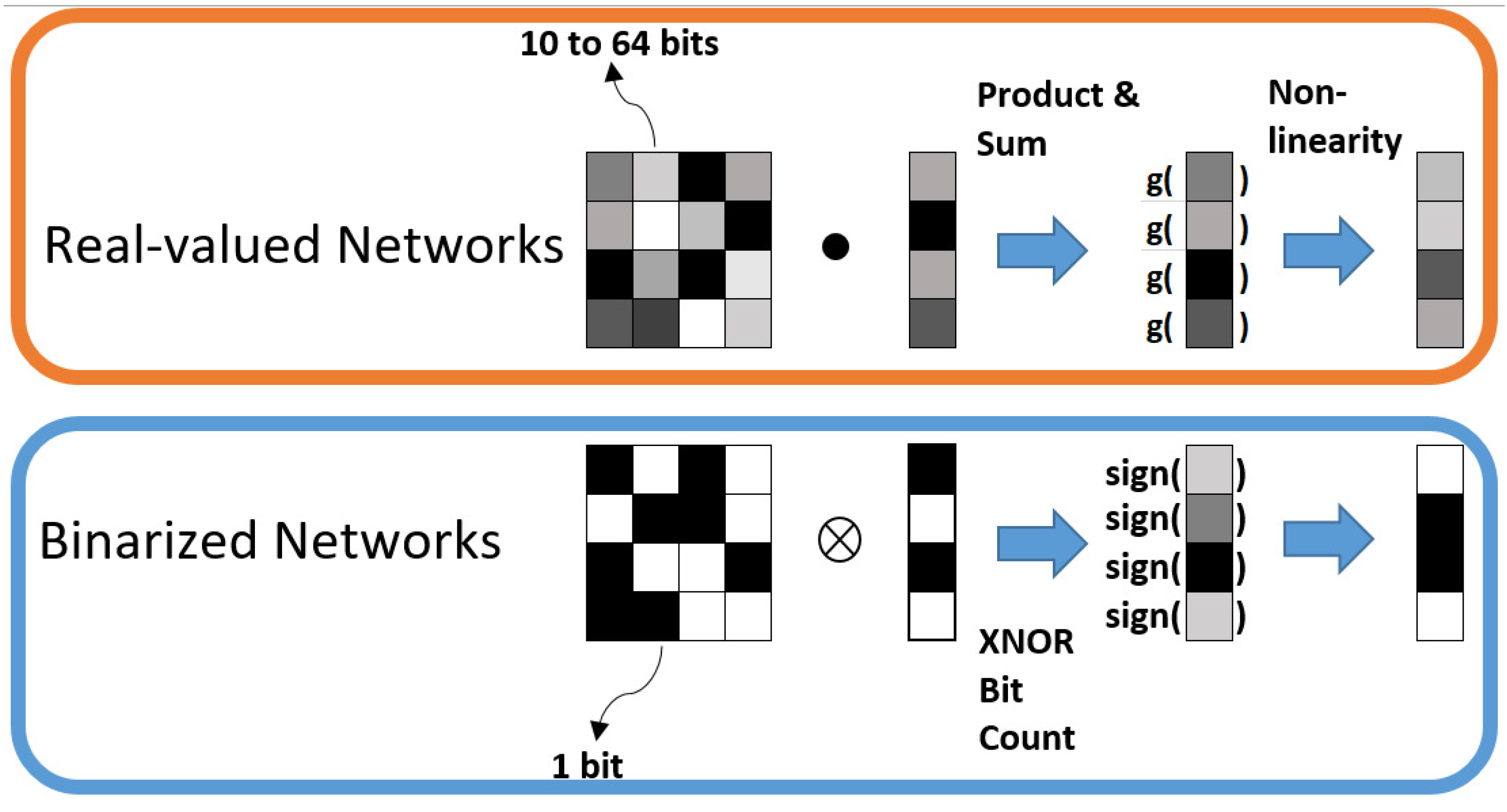Figure 1 illustrates the general difference between real-valued and completely binarized neural networks.

While real-valued networks are based on multiplications and accumulations, these calculations are replaced by simple XNOR operations and a bit count. The output of the XNOR operation is true when both bits have the same sign and false otherwise. Afterwards, the number of set bits is counted. A detailed overview of the involved operations can be found in [29]. The quantization of the weights and the activations is essential for the function of BCNNs. Quantization means the process of constraining continuous values to a discrete set with a finite number of elements. We use the following quantization function, which quantizes a real number $r_i\in [0,1]$ to a number of k bits $r_0\in [0,1]$ according to [24]:

$$quant\left(r_i\right)=r_0=\left\{\begin{array}{cc}0\hfill & if{r}_i<0\hfill \\ 2^k-1\hfill & if{r}_i>2^k-1\hfill \\ round\left(r_i\right)\hfill & else\hfill \end{array}\right.$$

(1)

To obtain the quantized weights for our neural network, we apply the equation:

$$f_w^k\left(r_i\right)=2\times quant\left(\frac{tanh\left(r_i\right)}{2\times max\left(\right|tanh\left(r_i\right)\left|\right)}+\frac{1}{2}\right)-1$$

(2)

Using a bit width of one reduces the function to:

$$r_0=sgn\left(r_i\right)\times E\left(\right|r_i\left|\right)$$

(3)

i.e., we take the sign of the real-valued weights and scale it by the scaling factor $E\left(\right|r_i\left|\right)$, which increases the value range. The resulting fixed-point integer allows the calculation of convolutions by means of fixed-point integer dot products, which can be performed on FPGAs in a highly efficient manner. For the quantization of the activations, we apply the function:

$$f_a^k\left(r_i\right)=quant\left(r_i\right)$$

(4)

The parameter k represents the number of the bits that should be used for the quantization of the activation r. By means of that, a discrete set of values is obtained, which replaces the floating-point convolutions by bit convolutions.

The binarization of the weights and activation and thus the switch from floating-point to fixed-point arithmetic can be implemented by bit shifts and basic logic operations on an FPGA, which speeds the calculations up significantly while additionally saving logic gates. Since the first convolutional layer represents the interface to the image, we do not apply quantization to its weights. It was shown that the quantization of the first layer leads to massively degraded prediction accuracy. Hence, we keep the first layer weights real-valued to keep the balance between computation complexity and prediction accuracy.

2.2. Dataset

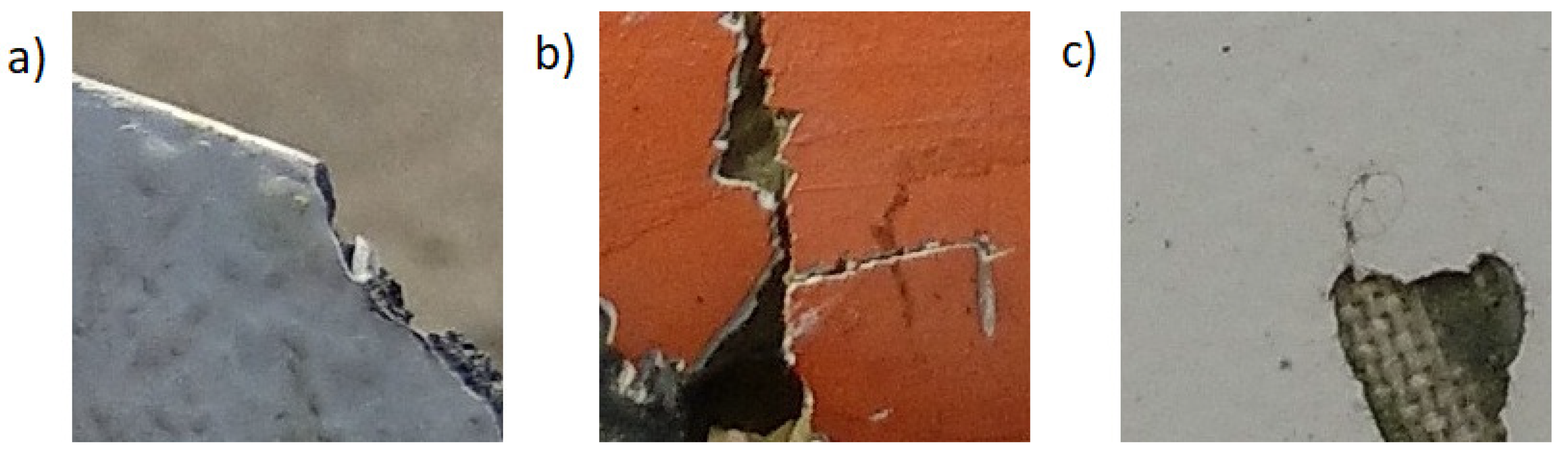
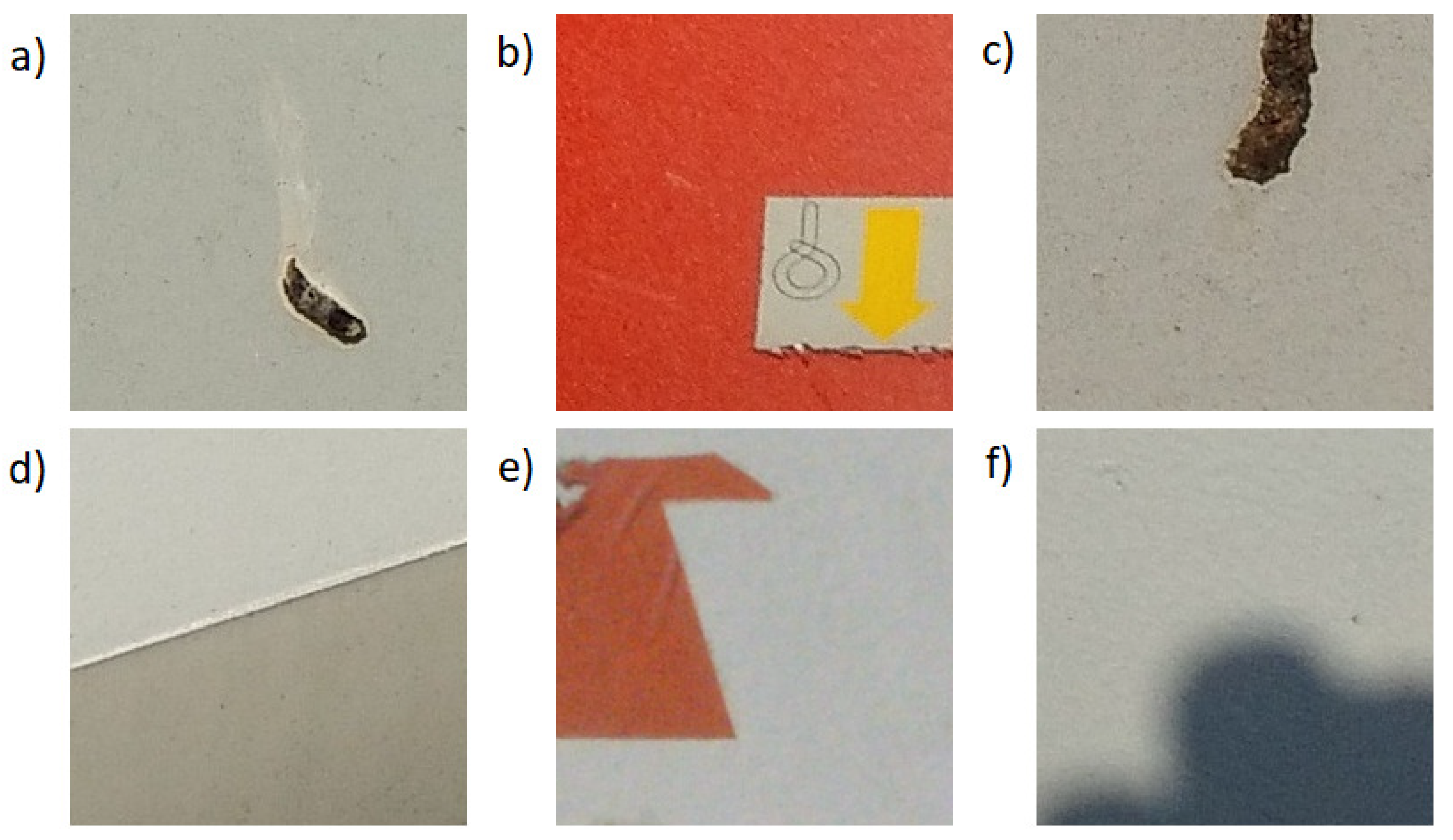
For our experiments, we built a dataset containing 1046 color images of different wind turbine rotor blades, taken at a resolution of $4608\times 3456$ pixels. From these images, we cut out windows of $224\times 224$ pixels containing relevant areas. This resulted in 8024 images of two classes: defective and non-defective. We included different classes of defects containing scratches, cracks, fractures and chippings. The defect types were selected by an expert to ensure a highly accurate differentiation between images of rotor blades with real defects and those which only seem to be defects. We did not classify the images into different classes but only into defective and non-defective ones. For each class, there are equal numbers of samples, i.e., 4012. To ensure proper training of all relevant scenarios, we oversampled difficult cases such as bird droppings, markings and color changes. Figure 2 and Figure 3 show different samples for each of these two classes. To limit the resource utilization of the FPGA, we converted the images to $80\times 80$ pixels and averaged the three color channels to one grayscale channel.

During the training, we applied different techniques for data augmentation, which have been shown to increase model accuracy. We implemented this by using the AugmentImageComponent class of the training interface Tensorpack based on Tensorflow. The interface allows a fast and flexible training of Tensorflow models by, e.g., providing classes for dataset streaming and data augmentation. We set-up a list with the parameters shown in

Table 1. Augmentation parameters.

Parameter Name	Parameter Value
Horizontal flip	True (probability 0.5)
Vertical flip	True (probability 0.5)
Transpose	True (probability 0.5)
Shift	Horizontal and vertical fraction 0.2

.

The parameter values for the horizontal and vertical flip and the transpose were set to 0.5 to augment the images with a probability of 50%. The horizontal and vertical fraction parameters for the shift augmentation were set to 20% so that not too much of the image content is lost. Since most of the defects are located in the center of the images, this value is appropriate.

2.3. Neural Network Configuration

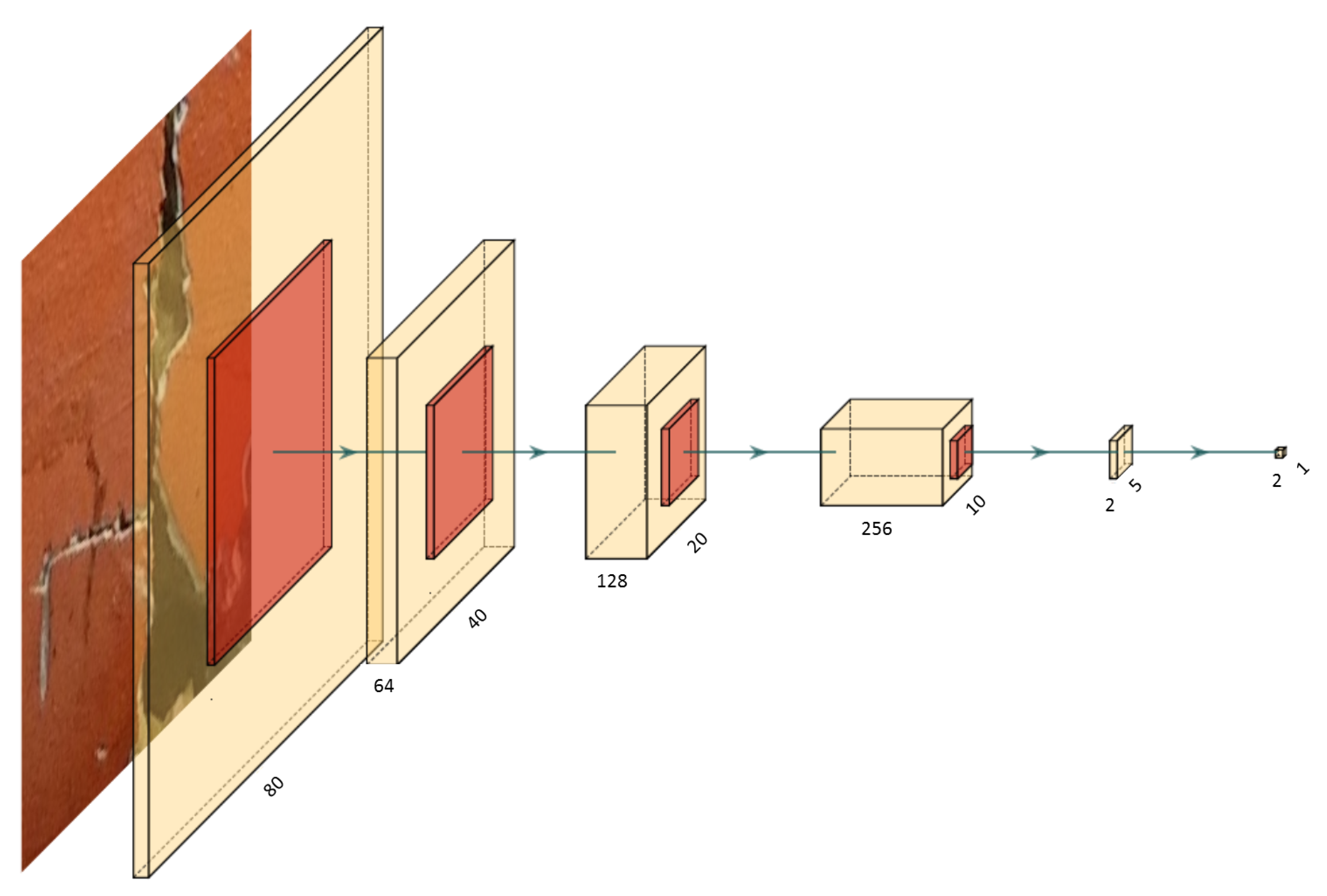
In the first step of the development of the binary neural network, the Convolutional Neural Network model was described in software, where we used Tensorflow as Python-framework. We implement ed a structure according to Figure 4. Five convolutional layers followed by max-pooling layers reduced the image size from 80 × 80 pixels and one channel (grayscale) to a feature tensor of dimensions 5 × 5 × 256. In the last convolutional layer, the feature maps were reduced to two channels to represent the two detectable classes. In the end, a global average pooling was applied to the two channels followed by a softmax layer to get the probability for each class of the image input. In that way, fully-connected layers, which are commonly used as the last layers for the classification task, were kept out of the network. These are much more memory-intensive than convolutional layers, and, by avoiding them, a great part of the FPGA memory could be saved for other operations such as additional convolutional layers or a higher number of feature maps.

The network size was restricted due to the limited amount of block RAM of the FPGA. More neurons and layers lead to more parameters that have to be stored. As common for classification tasks, we used the sparse softmax cross-entropy as a loss function to be minimized and the ADAM optimizer as an optimization algorithm [30,31]. Among the hyperparameters that define the training of a neural network, the learning rate is one of the most important. Several recommendations for the optimal learning rate were proposed in different publications, while it is mostly stated to be chosen between ${10}^{-6}$ and 0.1 [30]. Instead of using standard parameter values, the authors of [32] developed a systematic approach for finding the optimal one by sweeping the rate from a small lower to a high upper bound and by plotting the loss development. Figure 5 shows the result of that technique applied to our dataset. The optimal learning rate range can be found at the steepest slope of the plot, in this case between approximately $4\times {10}^{-5}$ and $9\times {10}^{-5}$. Below that range, the loss decreases at a very slow rate, which would lead to a too long training time. A higher learning rate than the upper bound of the optimal range causes an increase of the loss and a divergent and unstable behavior. Due to these results, we set the initial learning rate of our training to $9\times {10}^{-5}$ and applied a step decay function to it, which dropped the rate by a factor after a particular number of steps. The equation of the learning rate decay can be represented by:

$$learningrate=learningrat{e}_{initial}\times dro{p}^{\lfloor \frac{1+epochs}{decaystep}\rfloor }$$

(5)

where the quotient $\frac{1+epochs}{decaystep}$ states after how many training steps the decay should be applied. The brackets $\lfloor \rfloor$ represent the floor-function that gives the greatest integer less than or equal to a given real number. We chose a drop of 0.1 and a decay every 50 epochs.

The correct quantization of the neuron weights and their activation functions is essential for the quality of the neural network. Quantization means the digitalization of analog floating-point values; in this case, the analog values are represented by the weights and activations. We evaluated the performance of different weights and activation quantizations and chose the best compromise between accuracy and computational complexity for our final model. The first convolutional layer was left real-valued without quantization at first due to the important role within the feature extraction and quantized in a second step to see if we could get reliable results in that way.

2.4. Training

The training and validation of the binarized neural network were performed within the Python environment on a PC equipped with an NVIDIA GeForce GTX 1060 6 GB. To ensure that our results are repeatable, we used k-fold cross-validation for each experiment. As a value of $k=10$ is most commonly used in the literature, we adopted that scheme, i.e., we split the data into ten equally sized subsets and used nine of the folds for training/validation and the remaining fold for evaluation [33]. The model accuracy was determined on the validation set using the weights after 120 epochs of training. This process was repeated ten times until each fold had served as evaluation data.

2.5. Field-Programmable Gate Arrays (FPGA)

FPGAs represent a type of integrated digital circuits, which can be loaded with logic circuits to perform certain tasks. These consist of arrays of logic blocks that can be interconnected with each other in different configurations to produce simple logic gates, such as AND, OR and XOR, more complex combinational functions or memory elements. The behavior of an FPGA is described directly through a hardware description language, e.g., VHDL (Very High Speed Integrated Circuit Hardware Description Language) or Verilog, or using high-level synthesis tools using higher programming languages such as C [34]. In comparison to microcontrollers, FPGAs work in parallel instead of a sequential manner. Thus, every computation within one clock cycle is performed at the same time without any time scheduling as is done by a CPU of a microcontroller, which can lead to massive speed gains for tasks benefiting from parallelism. Many modern machine learning tasks require high-performance hardware setups that imply high power consumption and hence are expensive to operate. FPGAs are known for their power efficiency and, because of that, have aroused interest from machine learning researchers within the last years, especially from those using neural networks [35].

To run a quantized neural network on an FPGA, the structure and weights have to be transformed into a bit-file, in which the logic gates are described to perform the desired task. The weights and activations of the layers calculated during the training are exported into a C-header-file and build, together with a C-implementation of the network structure, the final model for the hardware. Internally, the FPGA communicates with the Cortex A9 microprocessor over a 512-bit wide Advanced eXtensible Interface (AXI) for data transmission between the two devices. Due to the gray-scaling of the input images, one pixel consists of 8 bit. To determine the maximal amount of pixels that can be transmitted in parallel, the following minimization problem has to be solved.

$$J=argmin(512-8x)\forall x\in \mathbb{N},x\le 64$$

(6)

with the constraint:

$$(height\times width)modx=0$$

(7)

Using a dimension of 80 × 80 pixels for our input images, we obtained a number of 40 pixels, represented by 320 bits, that can be transmitted over the bus within one clock cycle. The total number of clock cycles needed for one image transmission can be calculated by the quotient of the total number of pixels and the number of pixels transmitted per clock, which resulted in 160 clocks.

The input data are passed through the layers of the network by means of streams. Those layers consist of the necessary operations such as convolution, max-pooling or global average pooling. For a detailed overview of the particular algorithms, we refer to the work of Kaara [36]. For the transformation of the C-Code into the register transfer level (RTL) and the following bit-file generation, the Xilinx Vivado High-Level-Synthesis (HLS) environment is used to translate the network into the FPGA-specific configuration. We used ready-to-use Vivado HLS scripts to perform that task, which were provided by Kaara [36]. Those define, among others, the destination platform and the desired clock period. The generated RTL is represented by a so-called intellectual property (IP), which is afterwards instantiated in Vivado to create the final bit-stream. Additionally, a Tcl file describing the overlay needs to be generated, which can be directly exported from the Vivado project.

We configured the weights and activations of the network to be placed by the optimizer either in distributed or in block RAM to be more flexible with the memory utilization. During the transformation process, several optimizations were performed to meet the necessary parameters such as timing. The timing of the FPGA logic has to be kept as small as possible and directly influences the achievable clock frequency and hence the inference time of the classification. It has to be guaranteed that every connection between logic gates is short enough to transmit a signal within one clock cycle. Several constraints such as clock skew, the arriving of the same clock signal at different components at different times or propagation delay, i.e., the time of a signal to reach its destination, have to be taken into consideration. For detailed information on the optimization methodology, we refer to the work of Kilts [37].

3. Results

We carried out a test series consisting of 400 different weights and activation quantization combinations to find a good compromise between classification accuracy and computation complexity, and thus computation time. 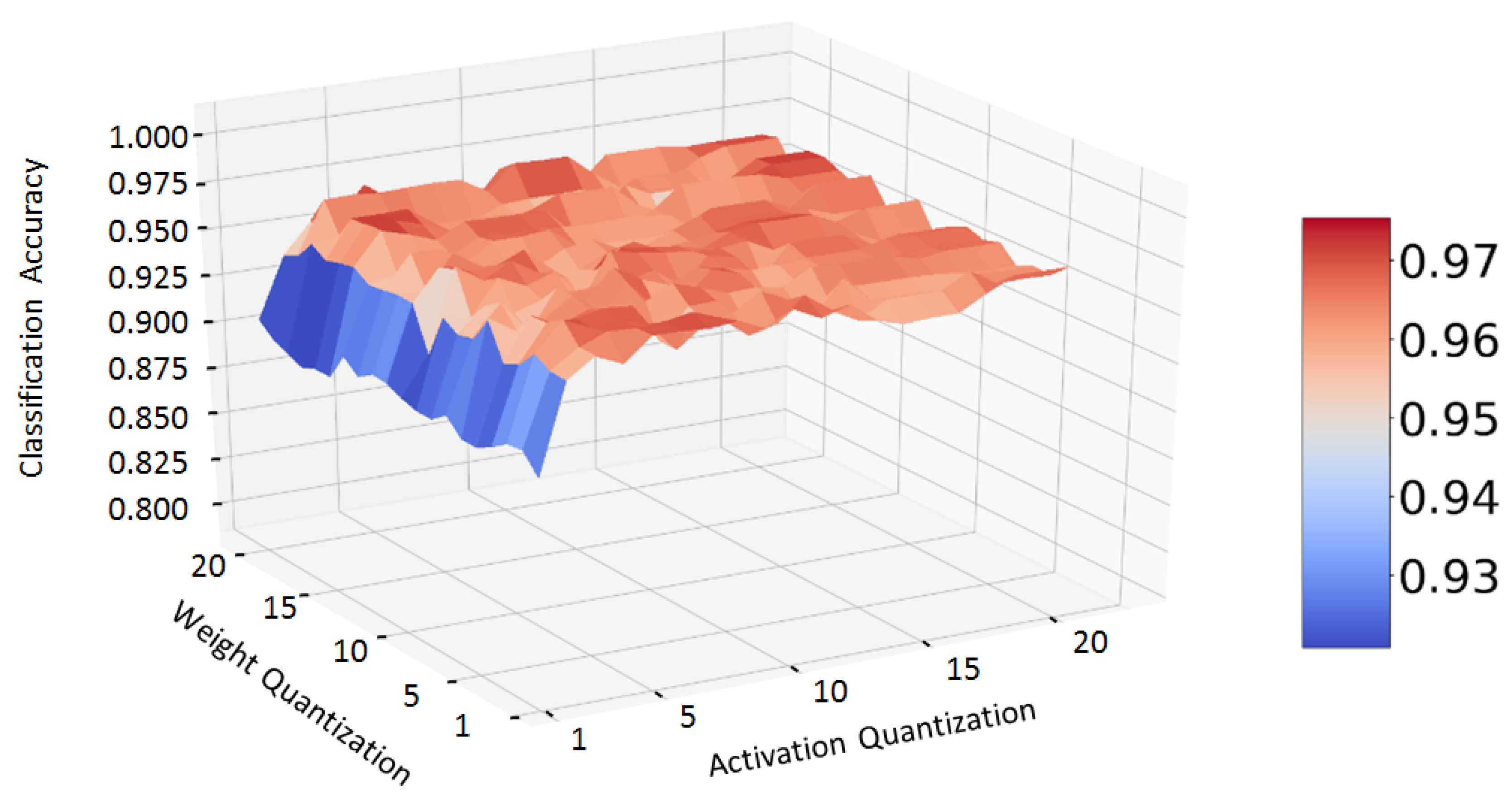The computation complexity of the dot product between two fixed-point integers, which is the basis of bit convolution, is directly proportional to the bit width of the two particular numbers [24]. Thus, the bit widths should be chosen as small as possible while keeping a good level of accuracy. Therefore, we trained the same network structure one after the other with quantizations reaching from 1 to 20 bits for weights and activations. Figure 6 shows the classification accuracy of our network tested on a test dataset depending on the bit width of weights and activation.

While the accuracy shows a high dependency on the number of bits used for activation quantization, the weight quantization seems to have no recognizable impact. As long as the bit width of the activations is greater than two, the classification accuracy remains approximately at the same level without improvement at higher bit widths. According to that result, we chose a quantization of 1 bit for the weights and three bits for the activations.

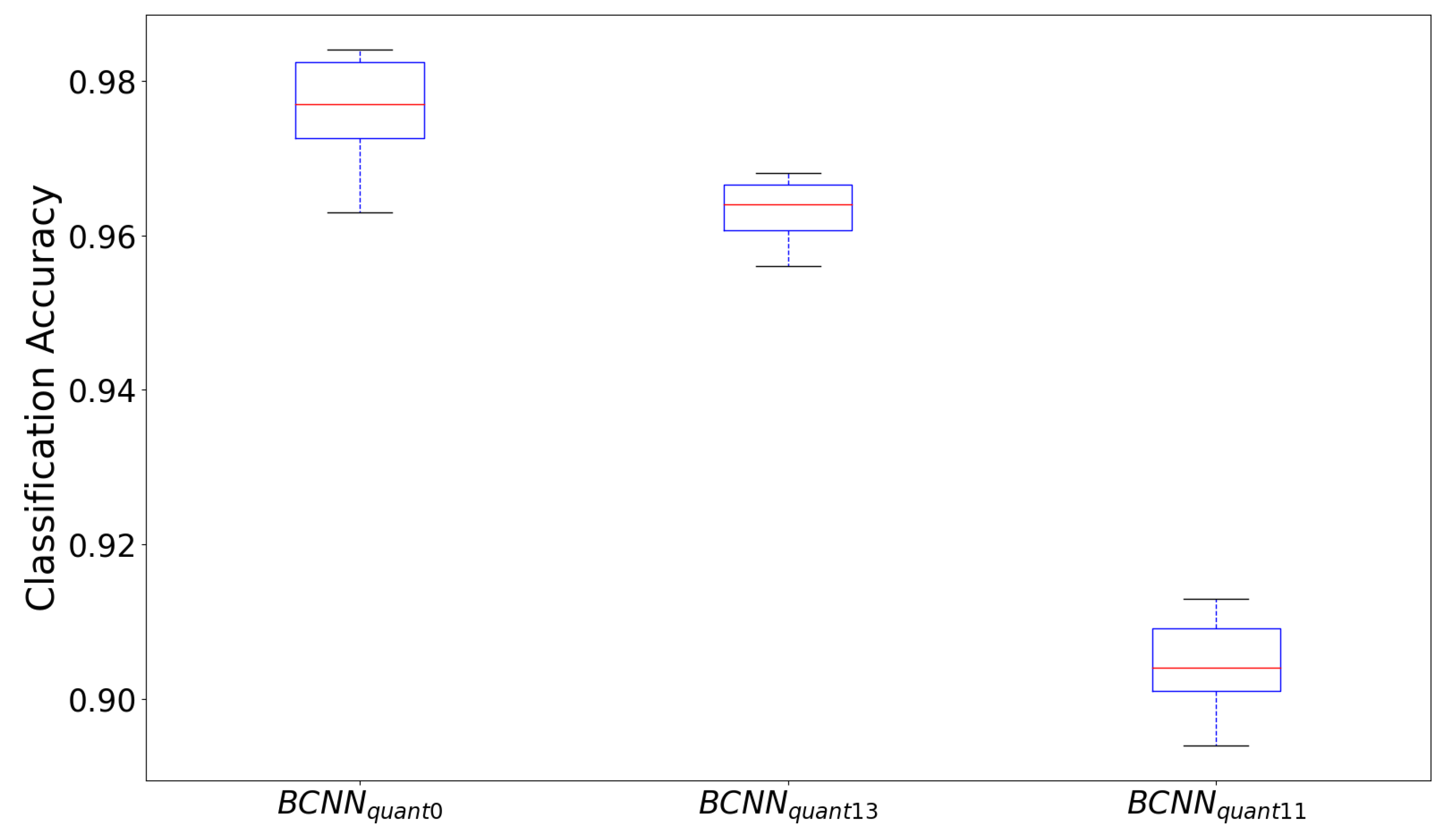
The results of the 10-fold cross-validation of the two network configurations are illustrated in Figure 7. The boxplot shows the comparison of the network with $80\times 80$ pixels input between the real-valued ($BCN{N}_{quant0}$), the 1-bit weight and 3-bit activation quantization ($BCN{N}_{quant13}$) and the 1-bit quantization for both weights and activations ($BCN{N}_{quant11}$) (from left to right). It can be observed that, as expected, the network $BCN{N}_{quant0}$ without quantization shows the best performance. The median of all folds is approximately 1 percentage point higher than the $BCN{N}_{quant13}$ ($97.7\%$ versus $96.4\%$). With a median of approximately $90.4\%$, the completely binarized network $BCN{N}_{quant11}$ performs worst during the cross-validation. It is noticeable that both the interquartile range (0.58% versus 0.94% [$BCN{N}_{quant0}$] and 0.81% [$BCN{N}_{quant11}$]) and the absolute range between maximum and minimum (1.2% versus 2.1% [$BCN{N}_{quant0}$] and 1.9% [$BCN{N}_{quant11}$]) of the network $BCN{N}_{quant13}$ with 3-bit activations quantization is the smallest among the configurations, which implies less dispersion over the folds.

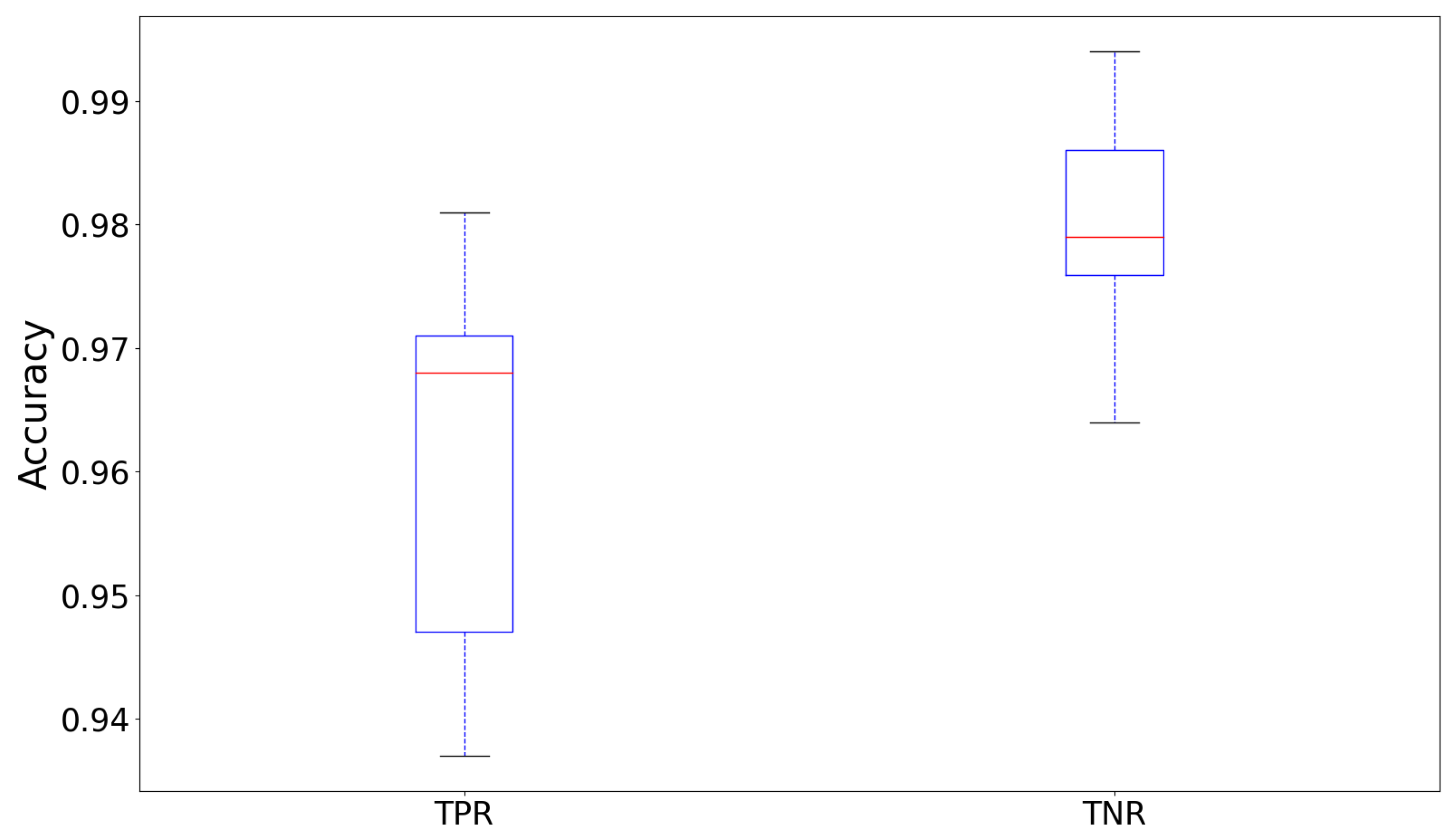
In conclusion, it can be stated that the network $BCN{N}_{quant13}$ shows the best compromise between calculation complexity and classification performance. We furthermore compared the true positive rate (TPR), called sensitivity and the true negative rates (TNR), called specificity, of the network $BCN{N}_{quant13}$ over the ten folds of the cross-validation, which is shown by the boxplot in Figure 8.

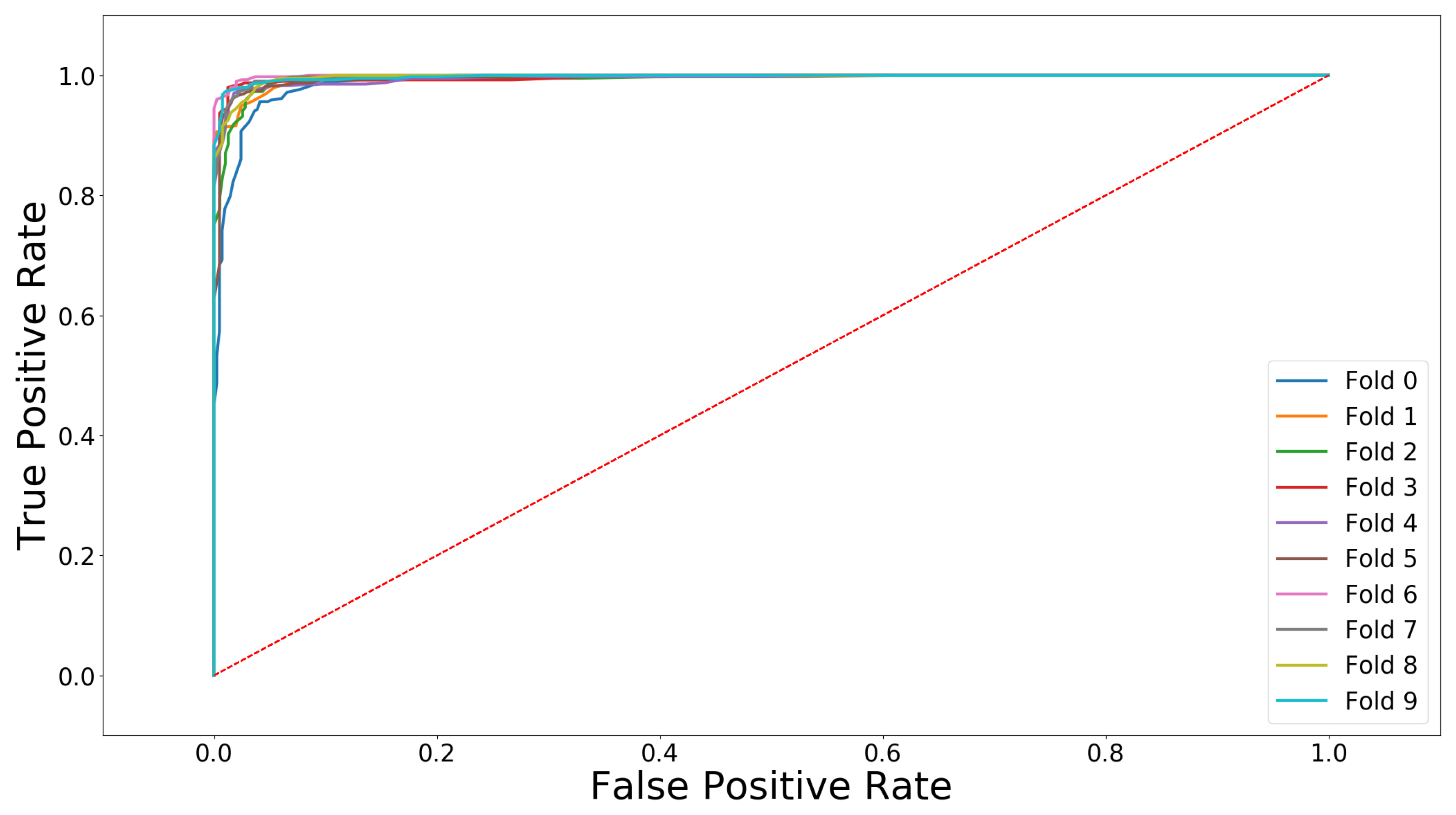
True positive in our case means a defect that was correctly detected, while a true negative means a correctly detected not defected input image. First, it can be ascertained that the median of the TNR is around 1% higher than the TPR ($97.9\%$ [TNR] compared to 96.8% [TPR]), which means that the classifier detects rotor blades without defects more accurately than it detects defected ones. The interquartile range of the TNR is furthermore approximately half the size of the TPR (∼1.1% compared to ∼2.3%) and also the absolute range of the TNR is much narrower (∼3.0% compared to ∼5.5% range). These observations mean that the TNR is more constant over the ten folds than the TPR. The receiver operating characteristic curves (ROC curve) in Figure 9 illustrates graphically the diagnostic ability of our classifier network over the ten folds. Thereby, the diagonal red line at 45 degrees represents a classifier that would do random guessing, also called the line of no-discrimination. Overall, our classification network shows the desired curve with a vertical rise at the beginning and near the upper left corner of the graph representing the perfect classification ($100\%$ sensitivity and $100\%$ specificity). The analysis of the ROC curve results in an optimal cut-point value, i.e., the optimal threshold for our classifier, which can mathematically be found by the highest Youden-index defined by [38]:

$$J=TPR-FPR$$

(8)

We calculate the median of the maximal Youden-indices of all ten folds resulting in a value of approximately $0.95$, which represents the median of the maximal vertical distance between the ROC curve and line of no-discrimination. The training of the completely quantized network reaches, as expected, a much lower accuracy of approximately $82\%$ and an unstable behavior during the training. A small learning rate has shown to be useful to prevent the loss function from diverging and from reaching stable values. We generate the bit-file for the FPGA with the weights and activations calculated during the training of the neural network with non-quantized first convolutional layer and otherwise 1-bit quantization for the weights and 3-bit quantization for activations. The resource utilization can be seen in

Table 2. Resource utilization of $BCN{N}_{quant13}$.

Resource Type	Used	Available	Utilization (%)
Slices	11,172	13,300	84.00
Look-up tables	27,132	53,200	51.00
Block RAM	117.5	140	83.93
DSPs	84	220	38.18
MUXes	73	26,600	0.27

.

Slices represent the configurable logic blocks of the FPGA and look-up-tables store predefined outputs for every combination of input, which allows a fast calculation. The utilization amounts to almost $85\%$ and approximately $50\%$, respectively. Thus, not many resources are left for logic operations, which limits possible extensions of the network with the current configuration. Increased input size of the images would lead to more calculations being necessary and hence would cause exhaustion of resources. The Block RAM enables the possibility to save data and contains inter alia the weights and activations of the neurons. The utilization amounts to approximately $2/3$. The DSP (Digital Signal Processing) slices perform complex calculations and speed up the performance of the FPGA. Almost half of them are used by the network which leaves space for extension. It can be seen that almost no Muxes (multiplexers) are needed as they are avoided due to the binarized network structure. During the continuous test classification, we measured the median power consumption of the FPGA board utilizing a USB power meter Crazepony UM24C and observed a value of approximately 1.2 Watts. The currently leading low-power embedded platform NVIDIA Jetson AGX Xavier consumes up to 15 Watts on average during GPU-intensive operations, which is more than 10 times higher. Even though the power consumption of a drone setup is many times higher than the consumption of an embedded platform, over time the additional required power can have a noticeable impact. In our case, we use a drone with a power consumption of approximately 880 Watts, which leads to an average flight time of 18 min when using a 12000 mAh battery with an output voltage of 22.2 Volts (manufacturer specifications). By using a NIVIDA AGX as an image processing board with an average power consumption of 15 Watts including necessary cooling, the flight time would be reduced by approximately 1% compared to almost no loss with the FPGA board. An additional factor is the small weight of the FPGA board, which is, with a value of 70 g, approximately three and a half times lighter than the NIVIDA AGX.

We achieve an inference time of approximately 4.6 ms at a clock rate of 200 MHz, which means that approximately 217 images can be classified per second by our quantized convolutional neural network. Denhof et al. tested the inference times of different pre-trained neural network structures and found the best result with the VGG16 network with an inference time of approximately 26 ms, which is about five times higher than our result.

Table 3. Performance comparison.

Network Model	Inference Time (ms)	Accuracy (%)
$BCN{N}_{quant13}$ (FPGA)	4.6	96.4
$BCN{N}_{quant13}$ (Jetson)	6.9	96.4
VGG16 (GPU)	26	97.0

compares the inference times and corresponding accuracies of the $BCN{N}_{quant13}$ run on an Nvidia Jetson AGX Xavier, the $BCN{N}_{quant13}$ run on a Xilinx XC7Z020-1CLG400C FPGA and the VGG16 implementation presented in [21] run on an Nvidia GeForce GTX 1060 TI.

Due to the deep structure of the VGG16 model, the inference time is approximately 5.6 times higher than our model run on the FPGA while gaining only six per mil in classification accuracy. The inference time of our model run on the Jetson is approximately $50\%$ higher than on the FPGA, which proves the speed improvement of our system.

4. Conclusions

In this paper, we present an FPGA implementation of a quantized convolutional neural network for the detection of surface defects on wind turbine rotor blades. Through that, we show that the classification accuracy on our dataset compared to a real-valued neural network with the same dimension is only slightly reduced. We obtain promising results with grayscale images and low resolution of $80\times 80$ pixels and a network with few layers, which can be optimized to increase the accuracy and probably to reduce the inference time, which is already low compared to an Nvidia Jetson AGX. By using bigger devices, e.g., the Xilinx XC7Z100 FPGA, much deeper neural networks could be implemented to achieve a higher accuracy similar to those running in software. Conceivable is also a connection of multiple FPGAs and the distribution of the network layers over them. By using techniques of the so-called ensemble learning, such as bootstrap aggregation or boosting and meta-ensembling, called stacking, high-performance neural networks could also be built despite the limited FPGA resources [39]. Thereby, small classifiers, with low performance on their own, can be clustered together to create more powerful networks. Generally, it can be said that the classification accuracy and the inference time are still improvable. Much higher performance with much lower inference time might be possible by optimizing the timing closure. That can be achieved by focusing on the optimization of the place and route algorithms of the network logic on the grid of the FPGA. If the inference time can be reduced to approximately 160 $\mathsf{\mu }$s, we can scan complete images of $1645\times 1234$ pixels by an $80\times 80$ grid in real-time with a frame rate of 20 fps. With the availability of higher clock rates, an optimized place and route routine, as well as generally a bigger device, the necessary low inference time could be possible.

Future work should also cover the differentiation between different kinds of defects instead of only distinguishing between good and defected rotor blades. Through that, particular repair methods can be organized and controlled. The use of FPGA-based machine learning platforms represents a promising alternative for mobile systems that have a limitation of power supply, due to the very low power consumption.