1. Introduction
In any scientific discipline where data usage is extensive, the provision of mathematical models that efficiently simulate a certain problem is a powerful tool that provides extremely valuable information. In economics, the study and use of econometric models that can simulate the relationship among many variables has been a key point in its development throughout the twentieth century. Nevertheless, in many cases, the computational cost has been an important drawback setting back the use of the largest models.
One of the most extended econometric models are Vector Autoregression (VAR) models [
1] which are multi-equation models that linearly describe the interactions and behavior of a group of variables, by using their own past. More specifically, a VAR is a particularization of a Simultaneous Equations Model formed by a system of equations in which the contemporary values of the variables do not appear in any explanatory variable in the equations. VAR models are traditionally used in finance and econometrics [
2,
3], but, with the arrival of Big Data, huge amounts of data are being collected in numerous fields like medicine, psychology or process engineering, giving to the VAR models an important role modeling this data. Although there are tools to tackle this issue, the large amount of data, along with the availability of computational techniques and high performance systems, advise an in-depth analysis of the computational aspects of VAR, so large models can be solved efficiently with today’s computational systems, whose basic components are nodes of multicore CPU plus GPUs.
There is ample literature on time series [
4], and, when the value of a variable at a time depends linearly on the value of one or more variables at previous instants, the structure of VAR is considered. In these models, there are dependent (endogenous) and independent (exogenous) variables. The first ones influence and are influenced by the rest of endogenous and exogenous variables. The second ones just influence but are not influenced, and are not predicted by the model.
To solve a VAR model, classical techniques like Ordinary Least Squares (OLS) (used equation by equation) or Maximum Likelihood estimator are commonly used. The practical challenge of its design lies in selecting the optimal length of the lag of the model. A general and actualized review can be seen in [
5].
Nevertheless, nowadays, an alternative point of view of VAR models is the Bayesian Vector Autoregressive models (BVAR), first proposed by Litterman [
6]. These models have become popular to deal with the overparameterization problem that appears in VAR models. In fact, BVAR models seem to be an alternative technique of the classic ones to estimate a VAR model.
Several recent articles survey the literature on BVARs. Koop and Korobilis (2010) [
7] propose a discussion of Bayesian multivariate time series models with an in-depth discussion of time-varying parameters and stochastic volatility models. As a recapitulation, S. Miranda and G. Ricco (2018) [
8] provide a review of ideas and contributions of BVAR literature.
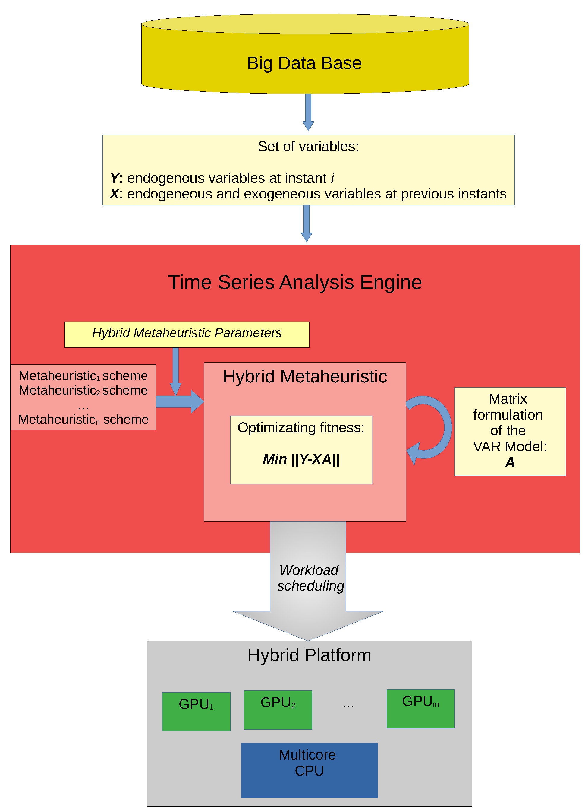
In summary, the main contribution of this work consists of the design and implementation of a high performance software engine for the estimation of VAR models by minimizing the difference between the dependent variables at instant
i, and the expression of their own past and the exogenous variables of the model. For the achievement of this general objective, it has been necessary to work in an interdisciplinary way in order to join a set of techniques, tools and paradigms of problem solving (
Figure 1):
A matrix formulation of VAR has been used, where, as will be described in detail in the following section, given a set of endogenous and exogenous variables (represent by Y and Z respectively), the endogenous variables at time i are expressed as a linear function of those endogenous variables in previous instants (, ,…) and the exogenous variables (both represented by X). Thus, the objective of the software is to find the coefficients of the model, represented by matrix A, which best represents the dependency of the VAR model; that is, that it better relates both data matrices Y and X. From a matrix point of view, this objective can be summarized in the minimization of the difference between the Y values and the values of the matrix multiplication . This matrix approach to VAR allows to apply high performance techniques in its resolution; that is, by becoming a problem of matrix calculation, several improvements has been introduced in the algorithms of resolution, such as the use of data block methods to optimize access to different levels of the hardware platform memory, with the consequent improvement of its performance. Likewise, the matrix vision of the problem allows the use of pre-optimized matrix libraries and an efficient execution of the software on high performance parallel platforms.
The problem of finding the optimum VAR model for a given series is an optimization problem whose solution can be approached through metaheuristics. The application of parameterized metaheuristic schemes has proved to be a practical approach for the determination of satisfactory metaheuristics for several problems [
9,
10]. Therefore, a flexible metaheuristic scheme has been used hybridizing it from a set of metaheuristics, both Local Search and population-based methods. A set of configuration parameters adjusts the degree of hybridization in each phase of the final metaheuristic scheme.
The parameterized metaheuristic scheme facilitates the development and optimization of parallel implementations [
11,
12]. The application of shared-memory parallelism to VAR is analyzed in [
13]. This work extends the proposal to heterogeneous parallelism so that shared-memory and CUDA parallelism are combined to fully exploit today’s computational systems composed of multicore CPU plus one or more GPU cards. In addition, for the distribution of workload between the different computing units (CPU and GPUs), different scheduling schemes (static versus dynamic, uniform versus balanced) are proposed and compared.
This high-performance proposal can facilitate tackling huge problems, with a large number of variables involved on which to study their relationships over long periods of time. In this way, in the last section of this paper, some previous results of the works that are being developing with scientists of several fields are shown.
The rest of the paper is organized as follows.
Section 2 describes the matrix formulation used in this paper. The hybrid metaheuristics considered for approaching the time series model are analyzed in
Section 3, while their parallelization for the exploitation of heterogeneous multicore+multiGPU parallelism is analyzed in
Section 4. The results of some experiments are shown in
Section 5.
Section 6 analyses possible applications of the parallel metaheuristics, and
Section 7 concludes the paper.
2. Matrix Formulation for Vector Autoregression Models
Considering
d dependent parameters at
t time instants, the vector of parameters at an instant
i is represented by
. Therefore, the time series
Y is a matrix of dimension
. Similarly, vectors
,
, represent the values of independent variables; each vector
is of size
e and the series of independent variables is a matrix
Z of dimension
. The values of the endogenous variables at instant
i depend on those of
and
previous instants for the endogenous and exogenous variables. The dependencies on the endogenous variables are represented by matrices
,
and those on the exogenous ones by matrices
,
:
where
C is a vector
of constant values.
They can be represented in matrix form, with the values of the series at instants
to
t depending on the previous ones:
Alternatively, if the vectors at previous instants are represented in a matrix
X of dimension
Equation (2) can be represented as
where the matrix on the right (built from matrices
,
and
C) represents the model of the time series. We call this matrix
A, of dimension
.
The optimization problem to be solved consists of the determination of the model (matrix
A) which best represents the dependencies on the time series:
The problem can be approached by Ordinary Least Squares (OLS). Here, basic Local Search and distributed metaheuristic algorithms and their hybridations are considered. The basic distributed metaheuristics are Genetic Algorithms [
14] and Scatter Search [
15], in combination with Local Search [
16] and Tabu Search [
17].
For each possible model (matrix
A, an element for the metaheuristic), the norm in Equation (5) represents the fitness. The time series,
, generated with the model represented by matrix
A and with the
initial vectors, is simulated with the multiplication
, with cost
, which means a high computational cost in the application of metaheuristics for large time series with large dependencies. Therefore, matrix computation techniques should be used to reduce the execution time [
18]. These techniques are not considered in this paper, which is devoted to the analysis of the application of hybrid metaheuristics and their parallelization on today’s multicore+multiGPU nodes. If optimized matrix operations were used, the execution time would be reduced, with no modifications to the metaheuristic, parallel schema.
3. Basic and Hybrid Metaheuristics
The representation of the candidate elements and their fitness are common to all the metaheuristics considered:
A candidate solution is a matrix
A (
,
and
C in Equation (4)) of size
. Different types of problems can be stated by imposing restrictions on the values in
A. For example, the values can be in an interval or a set of integers or real numbers. LAPACK [
19] can be used for the solution of Equation (5) for the real, continuous problem. The metaheuristic approach, generally with a larger execution time, can be used for the different versions of the problem. The results in the experimental section were obtained for solutions in an interval of real numbers, but this work focuses on the exploitation of parallelism, and the conclusions do not change significantly for different versions.
The fitness for a candidate solution
A is a measure of how the time series
Y is approached with model
A. The norm
divided by the square root of the number of elements of
Y (
) is used in the experiments. Other statistical criteria (Akaike (AIC) [
20], Schwarz (BIC) [
21], Hannan–Quinn (HQC) [
22], etc.) could be used, with different costs for the computation of the fitness. The differences in the solutions with the different criteria are residual, and now, again, the parallelism is not influenced by the fitness function.
Local Search methods work by analyzing the neighborhood of the candidate elements. The neighborhood considered for a vector with
entries consists of
elements, which are obtained by adding and subtracting a certain value to each position of the vector. If the best element in the neighborhood is better than the active element, it becomes the new active element. If not, the search continues with the same element, and the new neighborhood to be explored changes, due to the random generation of the neighbors. A maximum number of iterations from an initial value can be established and, after this number, a new active element can be generated for a new search. Therefore, a method similar to GRASP [
16] is obtained.
Tabu Search [
17] is used to guide the search. In our implementation, the last positions modified in the vector
v are maintained in the list. On the other hand, a long-term tabu strategy is used with a tabu element which is the mean of the best elements in a number of the last iterations. It is used in the selection of elements to be explored. Elements close to this tabu element are discarded.
The previous methods are Local Search metaheuristics, which can be hybridized with distributed metaheuristics. The most popular distributed (or population-based) metaheuristic is the Genetic Algorithm [
14], GA. The way in which the basic functions of the GA have been implemented is briefly explained:
Scatter Search (SS) [
23] differs from GA in the systematic application of intensification and in the way in which diversification is achieved. The main differences are:
Initialize: An initial set of elements is randomly generated as in GA, but it is normally smaller than for GA. The elements are improved before starting the iterations (hybridization).
Select: Typically, all the elements are combined, in pairs or bigger groups. In our implementation, the combination is like that for GA, but the percentages of best and worst elements selected for combination are similar, and a large number of combinations is carried out, and the elements so obtained are improved (hybridization).
Diversify: The diversification is carried out through the selection and combination of non-promising elements, and so mutation is not applied.
Include: The percentage of non-promising elements to be included in the reference set is now higher, again to help diversification.
Metaheuristics can be hybridized in many ways [
24], and hybridation with exact methods is also possible [
25]. Some hybridation possibilities have been mentioned for the basic methods considered. Metaheuristics can be developed with a unified schema [
26], which can in turn be parameterized [
9]. The parameterized schema used here for hybrid metaheuristics is shown in Algorithm 1. Each basic function includes some parameters whose values are selected to obtain basic metaheuristics or hybridations. The hybridation of Local Search and distributed methods is achieved with the inclusion of improvements in two parts of the schema.
| Algorithm 1: Parameterized schema for hybrid metaheuristics. |
| Initialize(ParamIni) |
| Improve(S_ini, ParamImpIni) |
while not EndCondition(S_ref, ParamEndCon) do Select(S_ref, ParamSel) Combine(S_sel, ParamCom) Diversify(S_ref, S_com, ParamDiv) Improve(S_com, S_div, ParamImp) Include(S_imp_com, S_imp_div, S_ref, ParamInc) end while
|
The metaheuristic parameters of the parameterized metaheuristic schema (Algorithm 1) are:
ParamIni (Parameters Initialize function): (Initial Number of Elements).
ParamImpIni (Parameters for Improving Initial Elements): (Percentage of Elements to be Improved in the initialization), (Intensification in the Improvement of Elements), (Length of the Tabu List for Local Search), (Final Number of Elements for successive iterations).
ParamEndCond (Parameters for End Condition): (Maximum Number of Iterations), (Maximum number of Iterations with Repetition).
ParamSel (Parameters for Select function): (Number of Best Elements selected for combination), (Number of Worst Elements selected for combination).
ParamCom (Parameters for Combine fuction): (Number of Best-Best elements combinations), (Number of Best-Worst elements combinations), (Number of Worst-Worst elements combinations).
ParamDiv (Parameters for Diversify function): (Percentage of Elements to be Diversified).
ParamImp (Parameters for Improve function): (Percentage of Elements obtained by combination to be Improved), (Intensification of the Improvement of Elements obtained by combination), (Intensification of the Improvement of elements obtained by Diversification), (Length of the Tabu List for Local Search on elements obtained by combination), (Length of the Tabu list for Local Search on elements obtained by Diversification).
ParamInc (Parameters for Include function): (Number of Best Elements included in the reference set for the next iteration), (Long-Term Memory size for the selection of elements to be included in the reference set).
The searching task of the most appropriate set of values for these parameters is a challenge in itself beyond the scope of this paper. One possibility to address it is by a hyperheuristic approach [
10], where this set of values can be selected so that it is suitable for the set of problems on which it will be applied, avoiding the dependence of each specific problem. A hyperheuristic can be implemented on top of the parametrized metaheuristic schema, searching within the space of metaheuristics determined by the values of the metaheuristic parameters.
4. Hybrid Metaheuristics on Heterogenous Multicore+multiGPU
Metaheuristics can be parallelized in a number of ways [
27,
28], and there are works on parallelization of each of the basic metaheuristics considered (Local Search [
29], Tabu Search [
30], Genetic Algorithm [
31], Ant Colony [
32], …), and for different types of computational systems (e.g., CMP architectures [
33], distributed platforms [
34] and GPUs [
35,
36]). On the other hand, the unified, parameterized schema enables the simultaneous implementation of parallel versions of different basic metaheuristics and their hybridations for different types of computational systems (e.g., shared-memory [
11], heterogeneous clusters [
12] and many-core systems like GPUs [
37]). In addition, when a hyperheuristic approach is included, a lot of metaheuristics are applied to different inputs, leading to a very large computational cost. Therefore, an upper parallel schema becomes mandatory to reduce execution times [
38,
39].
In shared-memory, parallelism can be implemented with independent parallelization of each basic routine in Algorithm 1. There are three parallelism levels:
The parallelization in the routines Initialize, Combine, Diversify and Include consists of just parallelization of a loop, with dynamic assignation of the steps of the loop to a pool of threads.
The improvement function has higher computational cost, and two levels of parallelism are used—the first to distribute the set of elements to be improved, and the second to assign different areas of the neighborhood to different threads.
Additionally, for our approximation to the time series problem, the matrix operations (matrix multiplication and computation of the norm) can be done in parallel.
The three levels are exploited in shared-memory with multilevel parallelism in OpenMP [
40], with a different number of threads at each level depending on the amount of work at each level and the characteristics of the computational system (number of cores and computational capacity). On the other hand, GPU parallelism can be exploited at different levels:
The highest level corresponds to an island schema, with the reference set divided in subsets which are each assigned to a different GPU. If only one GPU is available, all the computation should be carried out in that GPU.
The highest level of the shared-memory version corresponds to the parallelization of the loops for the treatment of elements. The steps of a loop are assigned to different threads, with one thread per GPU, and each thread calls its GPU to work with the corresponding element, which is transferred from the CPU to the GPU for the computation, and the required results (the elements generated together with the fitness) are transferred back from the GPU to the CPU. In this way the GPU computes the fitness of the element or explores its neighborhood in the improvement function.
GPUs can work at the second level of the shared-memory version: the analysis of the neighborhood of each element would be done in parallel, with each GPU working in one area of the neighborhood to obtain the best neighbor in its area, which is transferred together with its fitness back to the CPU, which computes the best neighbor before the next step of the improvement of the active element.
The parallelization at the lowest level would delegate the computation of the fitness to GPU.
In this work, a combination of the two middle-level versions has been considered. The GPUs work in the computation of the fitness after initialization, combination and diversification, and in the improvement of elements, where the parallelism at two levels might be explored (Algorithm 2).
| Algorithm 2: Parameterized schema for hybrid metaheuristics. CPU/GPU work distribution. |
| CPU: Initialize(ParamIni) |
| GPU: Computefitness(S_ini, ParamIni) |
| GPU: Improve(S_ini, ParamImpIni) |
while not EndCondition(S_ref, ParamEndCon) do CPU: Select(S_ref, ParamSel) CPU: Combine(S_sel, ParamCom) GPU: Computefitness(S_com, ParamCom) CPU: Diversify(S_ref, S_com, ParamDiv) GPU: Computefitness(S_div, ParamDiv) GPU: Improve(S_com, S_div, ParamImp) CPU: Include(S_imp_com, S_imp_div, S_ref, ParamInc) end while
|
Thus, taking into account this parallel schema, the method of finding the solution does not change in substance with respect to the CPU version, but now the work that is done with the components of these populations is distributed between the CPU and GPU threads. Therefore, the stop condition of the main loop is the same, thus maintaining the quality of the solution. Therefore, the experimental study of this work will focus on improving the speed of treatment of successive populations when multiple GPUs are used.
5. Experimental Results
Experiments were performed in 3 nodes with different CPUs and GPUs:
Marte: hexa-core CPU AMD Phenom II X6 1075T at 3.00 GHz, 16 GB of RAM. It includes a GPU NVidia GeForce GTX 480 (Fermi).
Saturno: 4 CPU Intel Xeon E7530 (hexa-core) at 1.87 GHz, 32 GB of RAM. It includes a GPU NVidia Tesla K20c (Kepler).
Jupiter: 2 CPU Intel Xeon E5-2620 (hexa-core) at 2.00 GHz, 32 GB of RAM. It includes 6 GPUs: 2 NVidia Tesla C2075 (Fermi) and 4 GeForce GTX 590 (Fermi).
Shared-memory parallelism is analyzed in [
13]. In general, the preferred number of threads at each of the three levels is different depending on the values of the metaheuristic parameters. Therefore, a different number of threads can be fixed for each level in each of the basic functions in Algorithm 1. The main conclusions in [
13] are summarized here:
The exploitation of parallelism at the highest level is, in general, preferred for small problems. The difference depends on the computational capacity of the node.
The performance with medium level parallelism decreases for small problems when the number of threads increases.
For large problems, medium level parallelism is preferred, especially when the number of threads increases.
The exploitation of low level parallelism is far worse than with the other types of parallelism.
In order to improve the global performance of the routine, the possibility of using GPUs has been studied to carry out the part of the work that best suits their characteristics. They can be used in different parts of the algorithm and with different levels of parallelism (Algorithm 2). Generally speaking, the use of these accelerators tends to offer better performance when they are responsible for solving computation-intensive parts of the problem, with a large number of operations on the same set of data and with an as uniform as possible operational schema. For this reason, the use of GPUs is centered mainly on the calculation of the fitness of each element: functions Computefitness and on the computation of the fitness inside function Improve. Different versions with different degrees of parallelism and schedule and balancing policies are considered:
The first version with one accelerator, called single_fitness_1GPU or sf_1GPU, consists of using a single GPU that performs the fitness calculations for each element (matrix multiplication and norm) one by one. It corresponds to parallelism at the third level in the shared-memory version, but in this case the computation of the fitness is delegated to the GPU.
The second version, called grouped_fitness_1GPU or gf_1GPU, seeks to increase the amount of data the GPU operates with, in order to optimize its use by addressing operations on large data sets. When calculating the fitness of the set of elements of the next generation that are children or neighbors (depending on the function) of the current elements, the set of individual multiplications is substituted by one multiplication by building a matrix composed of all the individual matrices to be multiplied. Therefore, parallelism works now at a higher level.
The first version for multiple GPUs, called static_uniform_scheduling_multiGPU or sus_mGPU, uses a static, uniform work distribution. The fitness calculations are distributed among the GPUs in the system without making decisions during the execution (static scheduling) and without taking into account possible differences in the performance of these accelerators (uniform scheduling).
The next version, called static_balanced_scheduling_multiGPU or sbs_mGPU, is a multiGPU version with static but non uniform distribution of the fitness calculations, where the quantity of work sent to each GPU is proportional to its relative computing capacity.
The last version, called dynamic_balanced_scheduling_multiGPU or dbs_mGPU, dynamically distributes the workload among the GPUs: the successive calculations of the fitness are scheduled, at runtime, among the different GPUs.
The use of two GPU matrix multiplication routines has also been considered in all the versions: a naive implementation and the multiplication routine in the CUBLAS library [
41].
The versions are compared in the nodes mentioned and for problems of variable sizes.
Table 1 shows the problem scenarios for the experiments. The names of the parameters are those used in the matrix formulation in
Section 2. The size of the multiplications when computing the fitness is also shown (
); it serves to compare the expected time for the different scenarios.
Different sets of metaheuristic parameters, which were introduced in
Section 3, have been tested, obtaining similar results in terms of the scope of this work (heterogeneous CPU+GPUs parallelization of the hybrid metaheuristic schema). The set of metaheuristic parameters used is:
ParamIni:
ParamImpIni: , , , .
ParamSel: , .
ParamCom: , , .
ParamDiv: .
ParamImp: , , , , .
ParamInc: , .
ParamEndCond: , .
That is, 80 elements are randomly generated, 50% of them are improved, with 10 steps of exploration of the neighborhood and a tabu list of only one element; the reference set for the successive iterations comprises 20 elements; the best 10 elements and 5 elements from the remaining ones are selected for combinations, with 10, 10 and 5 combinations between best, best-worst and worst elements; 50% of the elements in the reference set and those obtained by combination are improved, with intensity 10 and tabu list with 1 element; 20% of the elements are mutated, and the elements generated are improved with 20 steps of improvement and tabu list with 1 element; the 15 best elements and five elements from the remaining ones form the reference set for the next iteration; and information of the last 3 iterations is used to diversify the non-best elements selected.
For the experiments performed, a regular escalation in the execution times has been verified, independently of the number of algorithm main iterations. Therefore, each of the values that will be shown in figures and tables correspond to the average time of 20 executions, with 10 iterations per execution.
5.1. Experimental Results Using One GPU
In marte, with only one GPU, a version which only exploits CPU parallelism (
parallel_CPU or
pCPU) is compared with the two versions that use both the CPU and the GPU (
sf_1GPU and
gf_1GPU).
Table 2 shows the execution times of these versions for the problem scenarios in
Table 1 (the best time value for each scenario has been highlighted). As expected, as the problem size increases, the use of the GPU together with the CPU makes more sense, because the cost of the transfers from CPU to GPU is compensated by the exploitation of the computational power of the two units. Hence, for problem
, the execution times of all the GPU versions are similar, and larger than that of the CPU version. For larger problems (scenarios
,
and
), the times of the different versions that use GPU start to be lower than that of the parallel routine for CPU. The version
pCPU+gf_1GPU, which includes a global fitness calculation for a whole new generation of newborn or neighbor elements, produces a small improvement, which corresponds to how the operations performed are grouped. For the CUBLAS library, we can see in the first version (single application of each matrix multiplication) how its performance improves on those of the three-loop routine when the size of the problem grows. However, the version which combines the matrix computations shows similar performance when CUBLAS is used, which may be due to a larger cost of the CPU-GPU transfers.
Table 3 includes the same comparison for saturno. In this case, both the CPU and GPU are more powerful than in marte, although the costs of communication between the CPU-GPU memories are similar. For that reason, unlike in marte, GPU is not recommended for medium sized problems (scenario
), although the accelerator offers improvements in performance when the input problem is larger (scenarios
and
).
In jupiter, the CPU is more powerful than in marte, as it comprises 12 cores, and 6 GPUs, 4 of them similar in power to that of marte, and the other 2 usually offer better performance, although it depends on the specific operations/routines to be executed.
Table 4 compares, in jupiter, the execution times of the CPU and one-GPU versions. The GPU used is one of the fastest in the node. The execution time of the CPU version is reduced by about a half for scenario
and by about one third in
, both with the basic version of single fitness calculation (
pCPU+sf_1GPU) and when it includes calculation grouping (
pCPU+gf_1GPU). The latter is somewhat better, mainly when the size of the problem grows, as happens in marte and saturno. In both cases, in addition, the use of CUBLAS supposes an improvement of around 10% in the performance.
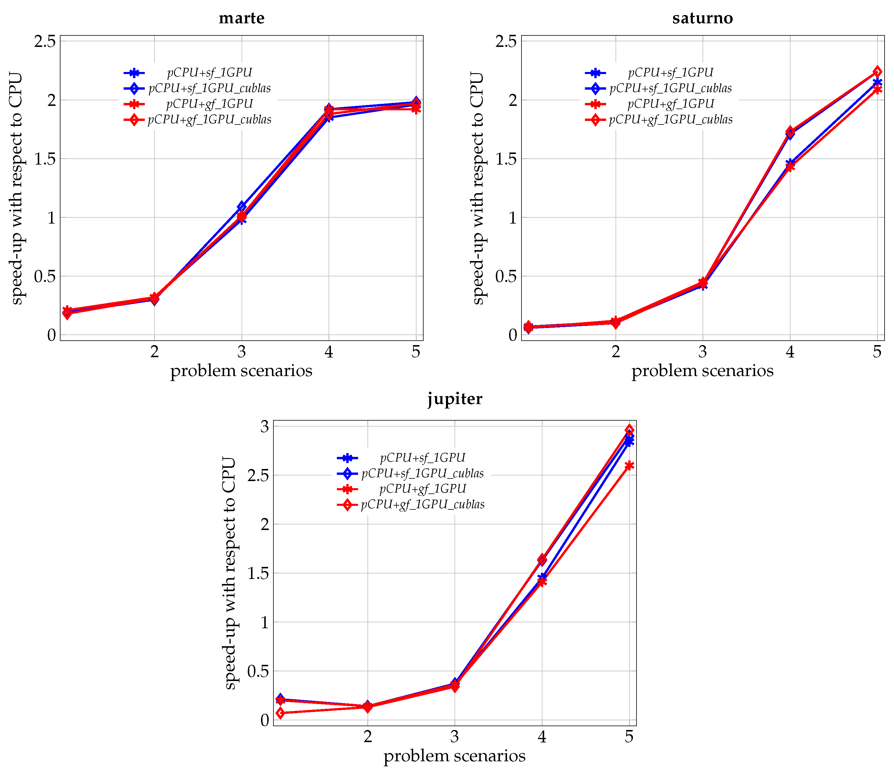
In
Figure 2, we can appreciate how, in the three hardware platforms and for all the CPU+GPU versions of the routine, the speed-up with respect to the CPU version clearly grows as we advance in the work scenario, which reaffirms the idea of the utility of the hybrid proposal, mainly as we face problems of greater dimension.
The differences in the behavior of the routines in the three nodes are due to the differences in relative CPU/GPU performance and in the cost of CPU-GPU transfers.
5.2. Experimental Results Using Multiple GPUs
The use of multiple GPUs can help to further reduce the execution time.
Table 5 shows the execution time of the different hybrid versions using multiple GPU with and without CUBLAS. Results are shown for the largest scenarios in
Table 1 (the best time value for each scenario has been highlighted; for each number of GPUs, the best time value for each scenario has been underlined). The main conclusions from the comparison of the results with the different scheduling methods are:
The simplest method, with a uniform and static work distribution (pCPU+sus_mGPU) gives satisfactory results for small problems and/or with few GPUs.
When the size of the problem grows and, mainly, with more GPUs, both the static balanced distribution (pCPU+sbs_mGPU) and the dynamic distribution (pCPU+dbs_mGPU) begin to show better behavior, outperforming pCPU+sus_mGPU in some cases. In general, it seems that scheduling policies that take into account the heterogeneous capacity of GPUs, either statically or dynamically, make more sense when the problem and platform grow in size and complexity:
- ∘
In the case of pCPU+sbs_mGPU, the size of the problem must grow so that the static balancing policy corresponds better to the relative performance of the GPUs.
- ∘
On the other hand, in pCPU+dbs_mGPU, the overload introduced by the dynamic distribution of work is compensated by achieving work distributions which are more proportional to the computational capacity of each process unit.
Figure 3 shows the evolution of the speed-up with respect to the parallel execution in CPU when the problem size increases, for the different hybrid versions and for different number of GPUs. In general, with multiple GPUs, greater performance is achieved, increasing with the size of the problem and the number of GPUs, and showing good scalability of the routine. For example, under scenario
, the performance generally improves when using more than 3 GPUs, while for scenarios
and
, a single GPU improves the CPU time, and the performance is multiplied up to
when the 6 GPUs are used. Although the growth of this value is initially less pronounced in those versions using CUBLAS, for the largest problem size it tends towards costs similar to the other implementations. This seems to indicate that when there are more GPUs in the system, CUBLAS needs even larger problem sizes, in order to have enough distributed work on each GPU to achieve better performance.
6. Ongoing Work: Possible Applications
Experiments have been carried out in five different problems obtaining five VAR models, three of them are classic economy problems, and the others two are from medicine. The time, the internal variables and the time dependencies are shown in
Table 6. No exogenous variables were considered. The cost of the multiplication
in Equation (5) is also shown. Therefore, there are big differences in the expected times for the different applications, especially for the data in the medicine application called
Neurology.
A brief description of these problems and the main characteristics of these applications are exposed:
Productivity corresponds to a classical economic problem of forecasting the Gross Domestic Product (GDP) based on the work of Gali (1999) [
42]. In this problem, data on productivity and hours worked spanning the period from 1983 to 2016 at quarterly frequency are used for the U.S. Given that GDP can be decomposed into productivity and hours worked, obtaining predictions of these two variables can be used as predictors of the GDP.
Interest is another classical problem used by economic researchers to predict the business cycle, i.e., expansions and recessions. The gap in the maturity of interest rates, also known as the yield curve, is a leading indicator of the business cycle behavior [
43]. We use monthly data for the one-year and the three-month interest rates from 1953M5 to 2005M7 for the U.S. in a VAR framework to assess this problem.
Product denotes a classical economic problem. In particular, is a monetary policy concern. Given that it is crucial to understand how monetary policy operates through the economy [
44], we evaluate this by using the following variables: industrial production as our economic activity variable, consumer price index as our price level variable, the one-year treasury bill rate as the monetary policy variable and the excess bond premium as our financial variable. We use monthly frequency from 1979M6 to 2018M2 for the U.S., taken from Datastream [
45].
Pressure corresponds to data of blood pressure (systolic and diastolic) and heart rate. Measures are taken during one day of a person’s normal daily life [
46]. Data from a population of patients are available. Only one patient is considered in the experiments, with measures taken approximately each 30 minutes in one day. The length of the dependency for the time series is not known, and two times are considered for the experiments.
Neurology is the biggest problem. Data came from the cerebral activity of a person. A helmet with potentiometers is used to register the answer of groups of neurons to some stimulus [
47]. It is not clear if a Multivariable Regression Model can be used to model the answers, so we are collaborating to detect patterns inside the large amount of data. Two time dependencies are considered in the experiments.
Experiments were conducted for these problems. In all cases, several executions (between five and fifteen, depending on the execution time) were carried out.
For the problems of Economy, the lowest fitnesses achieved are 0.4241 (
Productivity), 0.4553 (
Interest) and 0.3606 (
Product). These problems are classical examples of time series in economy, so it is not unusual to obtain satisfactory models. Here, the convergence greatly varies in time. While for
Productivity only 0.28 s of a Local Search method are needed, for the
Interest problem, the Local Search method runs for around 30.52 s and the time for
Product rises to 540.33. Experiments were carried out in a multicore with 12 cores, so for
Productivity, which is a very small problem, the sequential version of the algorithm was used, and for the other problems, with a similar size to the small problem in the figure, the shared-memory version with parallelism at the second level and with four threads was used.
Figure 4 shows the evolution of the fitness for the three problems, each 0.01 s for the first problem, each 1.5 s for the second and each 25 s for the third. For all three problems the convergence was satisfactory.
We are working on the application of techniques traditionally used in econometrics to medical data. For the Pressure problem, the best fitness obtained was 5.7212, in around 35 s. Thus, the model obtained is not as satisfactory as the fitness obtained in the economy problems. The data of only one patient were used, with a time dependency of two instants. The application of the software presented here to this problem needs to be carefully studied in collaboration with specialists in this field. Some possibilities are to consider several patients for the determination of the model, the analysis of the number of time dependencies, the classification of patients using their model, the study of pathologies represented by anomalous models, etc.
In the last problem, the computational system needs to be fully studied to be exploited, including multiple GPUs and linear algebra libraries, as it has been shown in the previous section. In any case, the initial experiments show a convergence of the metaheuristic similar to that in
Figure 4, but at much higher values than for the other problems. Collaboration with specialists in the field is needed to analyze, for example, the number of time dependencies and the variables to be considered.
7. Conclusions and Future Work
A matrix formulation for Vector Autoregression Models has been stated together with the basic and hybrid metaheuristics for the determination of satisfactory models. Parallel versions of the metaheuristics for multicore+multiGPU are studied. In shared-memory, three-level parallelism obtained with parallelism in the metaheuristic schema and in the matrix operations allows us to experiment with different combinations in order to obtain the best configuration according to the problem size, the values of the metaheuristic parameters (the metaheuristic being applied) and the computational system. For large problems, GPU parallelism can be used to reduce execution times, and the heterogeneity needs to be exploited to fully exploit the computational capacity of today’s multicore+multiGPU nodes. In these platforms, it seems that scheduling policies that take into account the heterogeneous capacity of GPUs offer better results when the platform grows in size and complexity.
Preliminary results show that the hybrid metaheuristics can be applied to obtain VAR models for series of data in different fields. The methods analyzed do not guarantee satisfactory models, but can be used in collaboration with scientists in these fields to analyze large amounts of data.
More research is needed to further reduce the execution time for large problems. The use of parallel matrix libraries needs to be optimized for the type and size of the problems on hand. Matrix computation techniques are being considered to improve the application of linear algebra routines, so reducing the cost of computation of the fitness and the overall execution time. For example, QR or LQ decompositions can be applied to simplify the model, and the Toeplitz-type structure in Equation (4) advises the adaptation of algorithms for structured matrices. Message-passing versions could be developed to solve the problems in larger computational systems composed of heterogeneous multicore+multiGPU nodes.

 ,
, 


