Underwater-Sonar-Image-Based 3D Point Cloud Reconstruction for High Data Utilization and Object Classification Using a Neural Network

1. Introduction

Object classification by autonomous underwater vehicles (AUVs) is necessary for various underwater missions, such as terrain-based navigation [1,2], target detection [3], and surveillance [4]. Because sonar sensors are robust to turbidity and have a long sensing range, AUVs are commonly equipped with a sonar sensor to perceive surrounding objects [5,6,7]. However, sonar sensors also suffer from a low signal-to-noise ratio (SNR) and low resolution. Therefore, various algorithms that can accurately classify objects even in noisy and low-resolution sonar data have been developed.

Such algorithms mainly represent sonar data as two-dimensional (2D) images and recognize objects using image processing techniques. Reed et al. [8] classified mines based on the shapes of shadows in sonar images. Kim et al. [9] proposed an object recognition method using Haar-like features, focusing on the fact that objects appear as a pair of highlights and shadows in sonar images. Recently, deep-learning-based algorithms have been introduced. Neural networks (NNs) extract and pool features from a large amount of data through deep layers, so they can accurately classify and detect target objects, such as docking stations [10], sea turtles [11], agent vehicles [12], and divers [13], even in noisy sonar images.

However, 2D-sonar-image-based algorithms have a drawback. Owing to the imaging mechanism of the sonar sensor, the shape of the object in the sonar image is affected greatly by the viewing angle. Because it is difficult to predict the direction from which the AUV approaches underwater objects, feature-based algorithms have limited accuracy. Furthermore, deep-learning-based algorithms require a large number of sonar images for training. Because open-source sonar data are scarce, underwater experiments should be conducted to capture training sonar images of objects according to viewing angles, which would require significant time and cost.

Therefore, methods to recognize objects using sonar images captured in multiple views have been proposed. Myer et al. [14] reduced object classification uncertainty by finding additional views that can increase the information of the object using the Markov Decision Process. Cho et al. [15] classified objects via template matching using images simulated according to viewing angles. Lee et al. [16] proposed an NN that classifies objects using eight sonar images taken at 45-degree intervals while rotating around the objects. However, these multi-view-based methods still face challenges. Considering all viewing angles along the roll, pitch, and yaw directions is difficult. They can also be challenging to apply to AUVs, which commonly have limited batteries, or to situations where rapid exploration is required.

To tackle the challenges of underwater object classification based on 2D sonar images, we herein propose a method to classify underwater objects by reconstructing their three-dimensional (3D) geometry. We generated 3D point clouds of underwater objects by extracting highlights from the sonar images of the objects that an AUV captured during a single fly-by scan. Then, the NN classified the objects using the restored 3D geometry.

The proposed method has the following advantages. First, the proposed method classifies objects more accurately than using a single 2D sonar image. The proposed method restores lost elevation information from consecutive sonar images and classifies the objects based on the reconstructed 3D geometry of the objects. Therefore, the proposed method can distinguish objects that may appear similar in 2D sonar images according to the viewing point. It is also robust to variation of highlight intensity depending on the environment in which the sonar image is captured. Next, the training process is straightforward. The training dataset for the proposed method can be synthesized directly from rough 3D models of objects, so additional underwater experiments to acquire training data, which require a lot of time and cost, are unnecessary. Finally, it is suitable for AUVs, which generally have limited operating times and computing power. The 3D geometry is reconstructed in a point cloud format—a set of $(x,y,z)$ coordinates—through a single scan by an AUV. Therefore, it does not require massive memory for storing data or complex computation for path planning of the AUV.

Using the proposed method, the AUV can create a 3D map of the underwater terrain and accurately recognize the map through classification. Additionally, the point cloud is a standardized data format for various terrestrial algorithms. Therefore, the proposed method can be applied to various AUV applications, such as simultaneous localization and mapping (SLAM), underwater investigation, and target object detection.

The remainder of this paper is organized as follows: In Section 2, we explain the difficulties of sonar-based underwater object classification. Section 3 describes the pipeline of the proposed method. Section 4 illustrates the experiments designed to verify the proposed method and present the experimental results. The paper ends with the conclusion in Section 5.

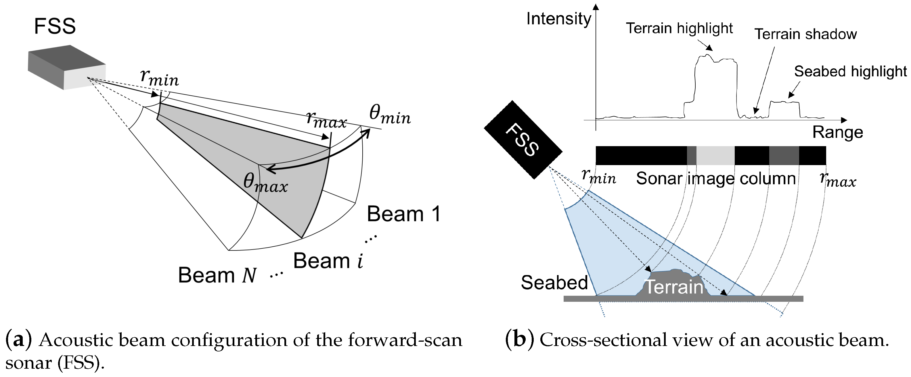
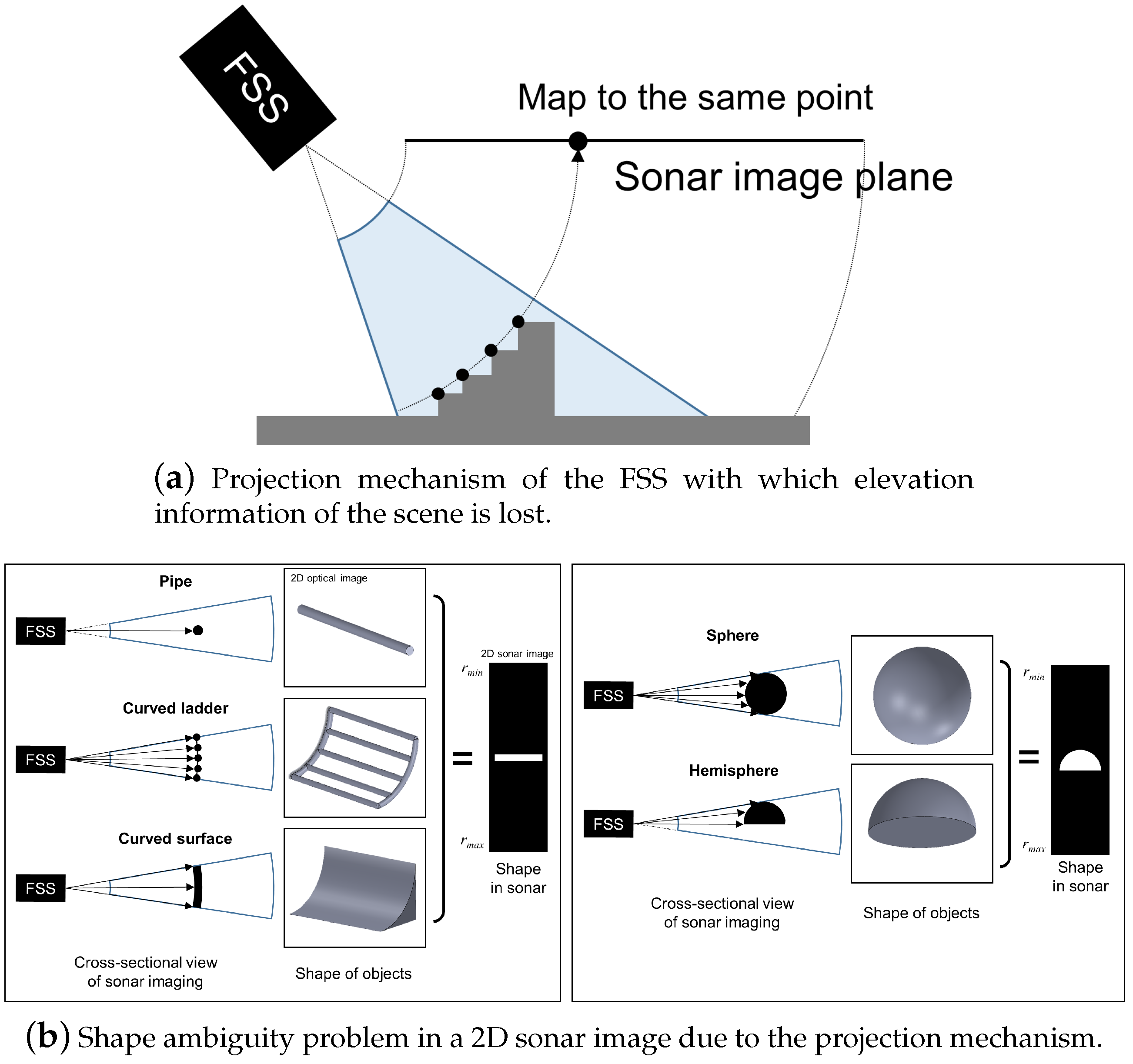
2. Problem Statement

Among various sonar sensors, we targeted a forward-scan sonar (FSS), which is widely used because it provides a relatively high-resolution images of its forward scene.

We first analyzed the principle of the FSS. An FSS senses its forward environment by transmitting acoustic beams and outputs it as a 2D image, as shown in Figure 1. The FSS consists of multiple acoustic transmitters and receivers to scan between the azimuth angles ${\theta }_{min}$ and ${\theta }_{max}$. For each azimuth angle $\theta$, a transmitter and receiver pair scans the range between $r_{min}$ and $r_{max}$ using an acoustic beam. Once a transmitter emits an acoustic beam, the beam is reflected from the surface of the underwater terrain and returned to the FSS. Then, its receiver measures the intensity of the returned beam according to the time of flight (TOF). The TOF represents the distance between the FSS and the underwater terrain from which the beam is reflected. The sonar image is constructed by mapping the measured intensity according to the corresponding distance and azimuth angle.

Object classification using a 2D sonar image has several drawbacks from its distinct imaging mechanism. First, the accuracy of the object classification can be seriously degraded according to the viewing point of the FSS, as shown in Figure 2. When the FSS projects the underwater scene, the elevation angle information of the underwater scene is lost because the FSS maps all points that have the same distance and azimuth from the sensor on an arc onto the same pixel, as in Figure 2a. As a result, depending on the viewing point of the FSS, objects with different shapes could all appear the same in the sonar image. For example, as shown in Figure 2b, a pipe, curved ladder, and curved shape can appear identical in 2D sonar images; a sphere and hemisphere as well. Furthermore, the shape and intensity of the same object change sharply depending on the viewing angle of the FSS and the underwater condition of capturing. Additionally, various vision-based algorithms have been developed on land, but such algorithms are hard to apply to a sonar image because the sonar imaging mechanism is different from the optical camera. The NN-based method is also difficult to use because the characteristics of sonar images are different from those of optical images, and there are not many open-source sonar image datasets.

This paper proposes a method to classify underwater objects by reconstructing the 3D geometry of the objects to tackle these difficulties of the FSS. The 3D geometry of an object provides more shape and dimension information compared to a 2D sonar image. It is also possible to generate base 3D models for the classification target readily, and then the object can be classified by comparing the restored 3D shape and the base 3D model at various viewing angles. The proposed method first restores elevation information lost when an object is projected onto 2D sonar images, and reconstructs the original 3D geometry of the object by analyzing consecutive sonar images while the AUV moves. Then, the proposed method classifies the reconstructed object using an NN. As a result, the proposed method can classify underwater objects more accurately through a more straightforward training process than classification based on a single 2D sonar image.

3. 3D-Geometry-Reconstruction-Based Underwater Object Classification

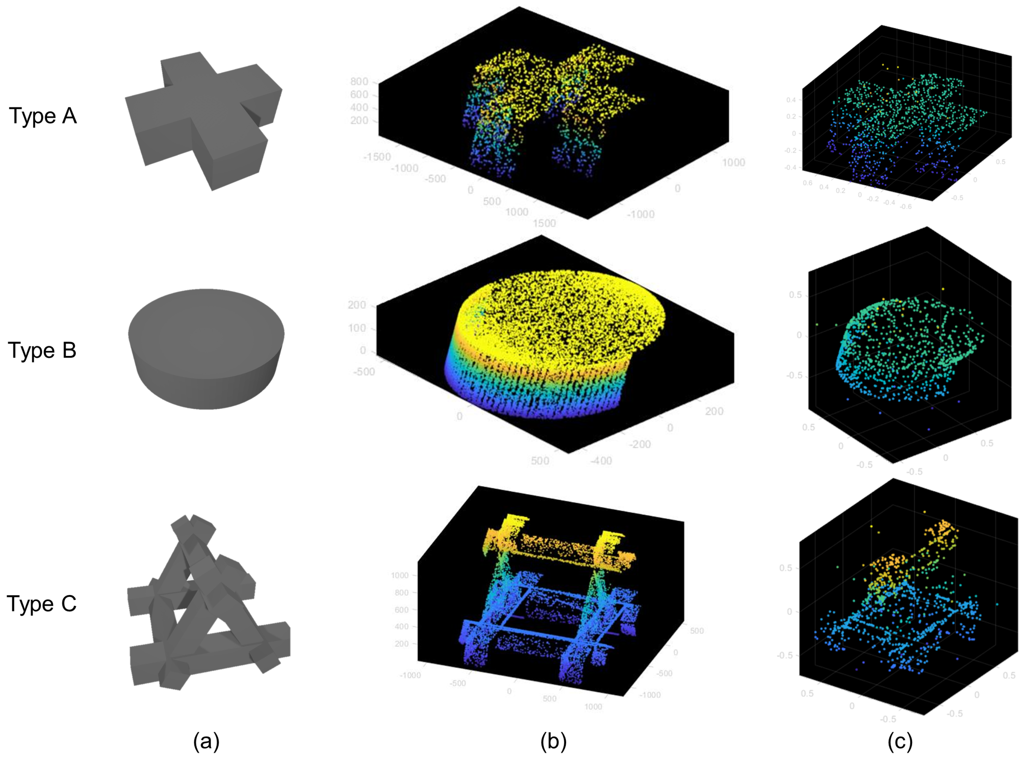
3.1. Target Scenario

Figure 3 describes the pipeline of the proposed method for classifying underwater objects. In the survey area, the AUV scans the seabed using the FSS while moving in a lawnmower trajectory, one of the primary methods of investigation of the AUV [17]. In the lawnmower trajectory, the AUV passes over the underwater objects covering the entire scan area. Then, by analyzing the captured sonar images as the AUV passes over an object, the 3D geometry of the underwater scene is restored in a point cloud. Because the sonar images have a low SNR and low resolution, the reconstructed point cloud is also noisy and sparse. Clustering removes the noise and extracts only the point cloud of the object. Finally, the NN predicts the class of the object from the extracted point cloud.

The proposed method can handle various difficulties of the sonar sensor. We address the 3D reconstruction of objects to classify underwater objects. Owing to the unique projection principle of the sonar sensor, the appearance of the object in the sonar image is largely affected by the viewing point. Sonar-image-based underwater object classification is problematic because it is nearly impossible to predict the angle at which the AUV encounters an object in an unstructured environment. If the object is restored in 3D, it is possible to classify the object more accurately by comparing the restored model with the 3D ground truth of the target object in various aspects.

For the classifier of the point cloud, we introduced an NN. The NN extracts and pools features through deep layers to enable robust classification from noisy and sparse sonar data.

Furthermore, the proposed method has a straightforward training process. When applying existing NN-based algorithms to underwater sonar sensors for their mission, the training step was one of the main challenges. The shape of the target object in the sonar images had to be predicted in advance, or a dataset consisting of many images had to be constructed through additional underwater experiments. On the other hand, because the proposed method classifies objects by restoring the object to its original form, the training does not require sonar images. Instead, it is possible to directly synthesize the training dataset from a 3D model of the object by reflecting the characteristics of the sonar sensor. As a result, the proposed classifier is easy to implement.

We propose using a point cloud when reconstructing the object in 3D from sonar images. There are several methods to represent the 3D model of an object, such as using voxels and meshes. The point cloud is a set of points with coordinate values of $(x,y,z)$; therefore, it does not consume much memory. Therefore, the point cloud is a suitable data format for the AUV, which has limited computing power. Additionally, the point cloud is a standardized format that is often used on land, so various terrestrial algorithms could be applicable for underwater operation.

The generated point cloud and classified object information can be utilized for AUV operations such as target detection and navigation. The remainder of this section explains the main elements of the proposed method in more detail.

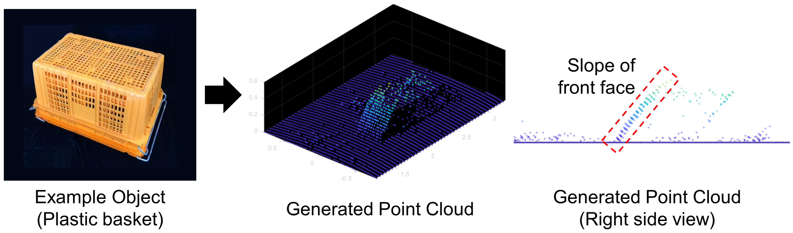
3.2. Reconstruction of the 3D Point Cloud of an Object Using FSS

For underwater object classification, the proposed method first reconstructed the 3D geometry of an underwater object using a sonar sensor. By restoring the 3D geometry using a point cloud, the AUV can accurately classify underwater objects without excessive memory overhead.

We could generate the 3D point cloud of underwater objects from a series of 2D sonar images. Cho et al. [18] developed a method to specify the elevation angle of underwater terrain by analyzing highlights in consecutively taken sonar images with an AUV, as shown in Figure 4. Although the FSS can scan a region between $r_{min}$ and $r_{max}$ in a single capture, the FSS has a sweet spot in which the strength of acoustic beams is concentrated and has the highest SNR. Therefore, when capturing an object by using an FSS, it is common to place the object in the sweet spot and make the seabed appear in the background, as shown in Figure 4a. On the other hand, Cho addressed an effect called highlight extension to restore the elevation angle of the object. As shown in Figure 4b, if the FSS approaches the object, the highlight extension effect occurs, in which the highlight of the object is observed before the seabed, since the object protrudes from the seabed. If the FSS approaches the object more, the length of the highlight extension increases until it reaches a critical position and does not change thereafter, as shown in Figure 4c,d.

The point cloud of the object can be generated using this highlight extension effect. Figure 5 shows the geometry between the FSS and the object at the critical position. Once the object reaches the critical point, the elevation angle of the object is specified as $t+s/2$ by the tilt angle of FSS t and spreading angle of beam s. Thus, the global coordinates of the highlight pixel of the object $[x_{obj},y_{obj},z_{obj}]$ can be calculated as

$$\left[\begin{array}{c}{x}_{obj}\\ y_{obj}\\ z_{obj}\end{array}\right]=\left[\begin{array}{c}{x}_{fss}\\ y_{fss}\\ z_{fss}\end{array}\right]+\mathit{R}\left[\begin{array}{c}{r}_c\sqrt{1-{sin}^2{\theta }_c-{sin}^2(t+\frac{1}{2}s)}\\ r_{c}sin{\theta }_c\\ r_{c}sin(t+\frac{1}{2}s)\end{array}\right],$$

(1)

where $[x_{fss},y_{fss},z_{fss}]$ denotes the position of the FSS, $\mathit{R}$ is the coordinate transform matrix from the FSS coordinate to the global coordinate, and $r_c$ and ${\theta }_c$ are the range and azimuth of the highlight pixel for which the 3D coordinate is to be calculated. Here, $[x_{fss},y_{fss},z_{fss}]$ and $\mathit{R}$ can be measured using navigational sensors of the AUV, and $r_c$ and ${\theta }_c$ can be calculated from the sonar image as

$$\left[\begin{array}{c}{r}_c\\ {\theta }_c\end{array}\right]=\left[\begin{array}{c}{r}_{min}+(r_{max}-r_{min})\frac{m}{M-1}\\ {\theta }_{min}+({\theta }_{max}-{\theta }_{min})\frac{n}{N-1}\end{array}\right],$$

(2)

where the size of the sonar image is M by N, and $(m,n)$ is the pixel coordinate of the highlight. Then, the point cloud of the object can be generated by accumulating the calculated coordinates of the extended highlights while scanning the object by utilizing the mobility of the AUV.

We pre-processed the point cloud for robust object classification. The pre-processing is to select only the points that belong to the object from the generated point cloud, and it consists of seabed removal and noise removal.

The points belonging to the seabed are removed first because the seabed is independent of the shape of the object. The raw point cloud is generated by analyzing highlights from the consecutive scene captured by the sonar image. The seabed itself also has highlights, so points corresponding to the seabed are also generated. However, according to (1), the z-coordinate of the seabed is calculated as near zero. We eliminated the seabed from the point cloud by filtering the points whose z values were smaller than a small threshold value.

Next, noise points that do not belong to the scanning target object are removed. Because the SNR of the sonar image is low, there is much noise in the point cloud generated from the sonar images. Additionally, even if the points with small z values are filtered, there may be natural features such as rocks and seaweed that have height. These points should be recognized as noise and removed.

To remove noise, we used density-based spatial clustering of applications with noise (DBSCAN) [19]. DBSCAN is a clustering algorithm that groups points based on whether there are enough neighboring points within a certain radius. The noise of the point cloud occurs from several highlight noise pixels of the sonar image, so points that do not have enough neighboring points could be considered as noise.

This method can generate point clouds of underwater objects in real time with less computation. Classically, 3D reconstruction from 2D images uses stereo vision. Stereo vision compares multiple images to find common areas or features, so it requires more memory and computation. On the other hand, this method generates the point cloud by calculating the height of an object slice that intersects the scan line whose elevation angle is $t+s/2$ while an AUV passes over the object. This approach does not require extraction of features, remembering previous images, or complicated path planning for AUVs. Therefore, this method is suitable for AUVs that operate in an unstructured environment and have limited computing power and batteries.

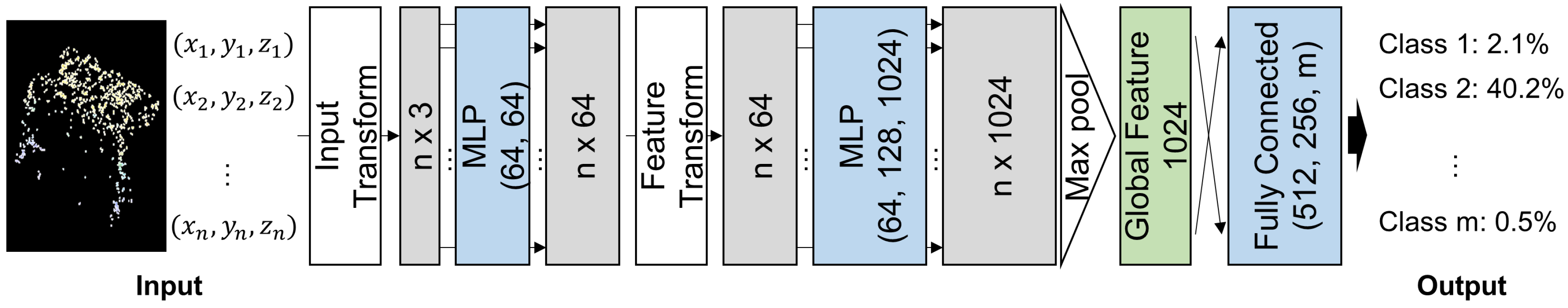
3.3. Object Classification Based on a Point Cloud Using PointNet

We introduced an NN to classify underwater objects with the generated point cloud of an object. As performance of GPUs has recently improved, NNs have been actively developed and exhibit an outstanding performance in object classification. Furthermore, a well-trained NN is robust to noise and environmental variation [20].

A point cloud is more advantageous than voxel or mesh in terms of memory [21], especially when reconstructing and storing a relatively small object in 3D using a sonar sensor with a large field of view and low resolution; however, it is difficult to extract meaningful information, since it is an unordered and unstructured set. An NN for classifying objects from a point cloud should have the following characteristics. First is the permutation invariance. Because a point cloud is a set of points that comprise an object, the NN should output the same result regardless of the order of those points. Second is the rigid motion invariance. The essential information of the point cloud is the overall shape and the distances among points. Therefore, transformations of the entire point cloud, such as translation or rotation, should not change the result.

From the NNs with these characteristics, we adopted PointNet [22]. Figure 6 illustrates the PointNet pipeline. The $(x,y,z)$ coordinate values of n points are input to the NN. For each point, PointNet extracts the local features of 1024 channels through multi-layer perceptrons (MLPs). Then, by applying max pooling to the extracted local features, a global feature vector representing the 3D shape of the point cloud is created. Finally, using this global feature vector, the NN can classify objects by predicting the score for each class through two fully connected layers.

In this pipeline, MLPs extracted local features independently for each point. Additionally, the max pooling operation is a symmetric function satisfying $f(x_1,x_2)=f(x_2,x_1)$, and is not affected by the input order. Therefore, PointNet satisfies order invariance.

Furthermore, PointNet applies transformations to the input point cloud and local features to meet the rigid motion invariance. The input and local features are transformed into canonical space by predicting the affine transformation matrix using mini-networks, which have an architecture analogous to the entire PointNet, and multiplying by the predicted matrix. These transformation steps can align inputs and extracted features, so the point clouds are classified as the same objects even if points are rotated and translated.

The PointNet is suitable for sonar-based underwater object classification. Because the sonar image is noisy and has low resolution, the point cloud generated from the sonar image is also noisy and sparse. However, PointNet can accurately classify sonar-based point clouds by extracting high-dimensional features through multiple layers. Furthermore, the PointNet has a simple and unified architecture consisting of few-layer MLPs, so the inference is calculated quickly and efficiently. Therefore, it is also suitable for use with AUVs.

Using the PointNet, underwater objects are classified as follows: An AUV generates a point cloud while the AUV passes over an underwater objects. For the input of PointNet, n points are randomly sampled from the generated point cloud. These points are then normalized to fit inside a sphere whose center is the origin and whose radius is one. Then, the object is classified by the inference of the PointNet.

3.4. Training Point Cloud Synthesis

Finally, we addressed a method to construct data to train the proposed underwater object classifier. A point cloud generated using a sonar sensor has two characteristics, which are different from those of sampling points directly from the polygons of the 3D shape of an object. We analyzed these two features for synthesized training point clouds from the 3D model of the object.

The first characteristic is the front slope, as in Figure 7. After the FSS reaches the critical point, the elevation angle is specified as $t+s/2$. However, from the beginning of the highlight extension until reaching the critical position, the frontmost and the uppermost point of the object, whose elevation angle is not $t+s/2$, is approximated to the point of the front surface. This approximation of the elevation angle causes the slope of the front face.

The front slope can be modeled by considering the displacement of the FSS in two consecutive sonar images when generating the point cloud [23], as shown in Figure 8. The sonar image is originally generated by projecting the points along the arc to the image plane, but it can be approximated that the points are projected orthogonally to the center plane of the sonar beam when the beam angle is sufficiently small. Then, if the FSS moves by $\mathsf{\Delta }{x}_{fss}$, the difference of ranges to the highlight pixel in two consecutive sonar images $\mathsf{\Delta }{r}_c$ is approximated as

$$\mathsf{\Delta }{r}_c\approx -\mathsf{\Delta }{x}_{fss}cost,$$

(3)

where t is the tilt angle of the FSS. On the $XZ$ plane of the FSS, the points of the front face in two consecutive sonar images i and $i+1$ are calculated as follows:

$$\left[\begin{array}{c}{x}_i\\ z_i\end{array}\right]=\left[\begin{array}{c}{x}_{fss,i}+r_{c,i}cos(t+\frac{1}{2}s)\\ z_{fss,i}+r_{c,i}sin(t+\frac{1}{2}s)\end{array}\right],\left[\begin{array}{c}{x}_{i+1}\\ z_{i+1}\end{array}\right]=\left[\begin{array}{c}{x}_{fss,i+1}+r_{c,i+1}cos(t+\frac{1}{2}s)\\ z_{fss,i+1}+r_{c,i+1}sin(t+\frac{1}{2}s)\end{array}\right].$$

(4)

Assuming that the FSS maintains altitude, $\mathsf{\Delta }{z}_{fss}$ is negligible. Then, from (3) and (4), the front slope is derived as

$$\frac{z_{i+1}-z_i}{x_{i+1}-xi}=\frac{costsin(t+\frac{1}{2}s)}{1-costcos(t+\frac{1}{2}s)}.$$

(5)

As a result, the front slope could be estimated from the tilt angle of the sonar. The generated point cloud can be corrected using the calculated slope. Alternatively, the network can be trained more robustly by adding the modeled front slope.

Next, the generated point cloud has limited surface information. The proposed method scans an object in a single direction to avoid overhead in the operation time of the AUV. Additionally, elevation angles can be specified only for the points reaching the critical position. Therefore, the points are reconstructed from the limited surfaces.

We proposed a method to detect the hidden surfaces that are not scanned according to the movement of the FSS, as shown in Figure 9. When the 3D model of an object is given, polygons facing the back based on the FSS are culled first. The scan direction vector $\overrightarrow{v_{fss}}$ of the FSS is specified as

$$\overrightarrow{v_{fss}}=(cos\psi ,sin\psi ,-tan(t+\frac{1}{2}s)),$$

(6)

by the heading of the AUV $\psi$, the tilt angle of the FSS t, and the beam spreading angle s. When the normal vector of a polygon of the 3D model is $\overrightarrow{N}$, if $\overrightarrow{v_{fss}}·\overrightarrow{N}\ge 0$, it means that the acoustic beam is not reflected from the polygon. Therefore, we removed those polygons from the given model.

Furthermore, points on the polygon could be generated when the polygon meets the scan line whose elevation angle is $t+s/2$ from the FSS. Hidden surfaces blocked by other surfaces could be removed by inspecting the collision between polygons and scan lines as the FSS moves.

We could construct a training dataset through the following process. When a 3D computer-aided design (CAD) model of an object is given, we first set a scan direction and remove the hidden surfaces. Then, points are randomly sampled from the remaining surface. By adding the estimated front slope through shear transformation, we could synthesize realistic training point clouds of target objects. In this way, because it is unnecessary to conduct actual underwater experiments to obtain the training data, the training process of the proposed object classifier becomes straightforward.

4. Experiment

To evaluate the proposed method, we conducted two types of experiments: a simulation experiment to verify whether the proposed method generates a 3D point cloud well for object classification and a field experiment that applies the proposed method to the classification of artificial reefs that have been installed in the sea. This section explains the data gathering, training, and experimental setup to test the proposed method and presents the experimental results for each experiment.

4.1. Simulation Experiment

A simulation experiment was conducted to verify the proposed point cloud generation and classification method. Figure 10 shows the steps for the simulation experiment. First, PointNet was trained using ModelNet40 [24]. ModelNet40 is an open-source dataset used as a benchmark for 3D shape classification. It consists of 12,311 mostly human-made 3D CAD models from 40 common categories, such as tables, chairs, and airplanes. We simulated the point clouds of these categories and checked whether the pre-trained PointNet could classify the point clouds.

4.1.1. Sonar Image Simulator

We used a sonar image simulator to generate the point cloud of the objects strictly according to the proposed method. There are several open-source simulators, such as the UUV Simulator [25] and Stonefish [26]. However, we developed a sonar simulator to customize well for the AUV and FSS in use. The sonar image simulator can be implemented by emulating the imaging mechanism of the sonar sensor analyzed in Figure 2a using ray tracing [27].

First, for the ray tracing of an acoustic beam with a vertical beam spreading angle, K rays were sampled between $t-s/2$ and $t+s/2$, where t is the tilt angle of the sonar sensor and s is the spreading angle. Given the 3D-modeled shape of an object, the simulator calculates the point of collision $\overrightarrow{p_{\theta ,k}}$ between the transmitted acoustic wave and the object as

$$\overrightarrow{p_{\theta ,k}}=\frac{\overrightarrow{N}·\overrightarrow{p_1}}{\overrightarrow{N}·\overrightarrow{v_{\theta ,k}}}\overrightarrow{v_{\theta ,k}},$$

(7)

where $\overrightarrow{N}$ and $\overrightarrow{p_1}$ are a normal vector and a position vector of the collided polygon of the given 3D model, respectively, and $\overrightarrow{v_{\theta ,k}}$ denotes the unit direction vector of the sample ray.

The sonar image is determined according to the TOF and intensity of the beam reflected from the collision point. Considering the transmission loss according to the distance of flight, material of the object, and Lambert’s cosine law [28], the intensity of the returned beam is modeled as

$$I_{p_{\theta ,k}}=w\frac{z-z_0}{z+z_0}\frac{I_0}{|\overrightarrow{p_{\theta ,k}}{|}^2}{cos}^2\alpha ,$$

(8)

where w is a constant for unit conversion, z and $z_0$ are the acoustic impedances of the object and water, respectively, $I_0$ denotes the initial intensity of the beam, and $\alpha$ is the angle between the sample ray and the collided polygon. The sonar image can be simulated by mapping the intensity to the corresponding range and azimuth angle as follows:

$$I(r,\theta )=\sum _{k\in \{\overrightarrow{p_{\theta ,k}}=r\}}{I}_{p_{\theta ,k}},$$

(9)

for $r_{min}\le r\le r_{max}$, ${\theta }_{min}\le \theta \le {\theta }_{max}$.

Finally, we added speckle noise to make the sonar image more realistic. Speckle noise is a typical noise of a sonar sensor caused by interference between acoustic beams and particles in water. By modeling speckle noise [29], the sonar image is synthesized according to the following equation:

$$I_{final}(r,\theta )={\left(\sqrt{I(r,\theta )}+\sum _{i=1}^{s(r,\theta )}{u}_i(r,\theta )\right)}^2+{\left(\sum _{i=1}^{s(r,\theta )}{v}_i(r,\theta )\right)}^2,$$

(10)

for $r_{min}\le r\le r_{max}$, ${\theta }_{min}\le \theta \le {\theta }_{max}$, where $s(r,\theta )$ is a random integer uniformly sampled within a range $[0,10]$, which is determined experimentally to make the output image realistic, and $u_i$ and $v_i$ are the real and imaginary parts of the acoustic beam phasors randomly sampled from the 2D Gaussian distribution.

The sonar image simulator can calculate the 2D sonar image of the given object from desired positions. We modeled four objects, such as bookshelves, doors, and stairs. Then, the sonar image simulator synthesized consecutive sonar images with changing positions along a predefined trajectory. Then, the proposed method generated point clouds from the simulated sonar images. For a precise verification, we simulated sonar images along three predefined trajectories and changed the tilt angle of the sonar simulator to 30${}^{\circ }$ and 45${}^{\circ }$ for each object.

4.1.2. Simulation Experiment Results

We confirmed the precision of the point cloud and the accuracy of the NN by classifying the generated test point clouds with the pre-trained PointNet. The point clouds were reconstructed using the proposed method from the simulated sonar images. Rotational transformations were also applied to the reconstructed point clouds to check whether the NN could classify objects invariant to rigid body transformation. In total, 82 test point clouds were generated. Then, using the test point clouds, the classification accuracy of the PointNet pre-trained with the terrestrial open-source dataset was measured.

Figure 11 shows the restored point cloud using the proposed method. Four objects were modeled in 3D using CAD, as shown in Figure 11a. The sonar simulator then synthesized consecutive sonar images by assuming a situation in which the AUV passed over the object, as shown in Figure 11b. Finally, the proposed method could restore the 3D point cloud of the objects, as shown in Figure 11c. Although the generated point clouds were sparse due to the low resolution of the sonar images and had undesired front slopes, the overall shape was reconstructed similarly to the original form of the object.

Finally, we measured the classification accuracy of the proposed method. For the quantitative results, the proposed method was evaluated using the precision and recall of classification. As a result, the precision recorded 91.7%, and the recall recorded 89.0%. PointNet classifies objects based on 3D geometry, so the high accuracy shows that the proposed method restores the essential 3D information of the object well. The proposed method generates a point cloud with only a single-directional scan, which is suitable for AUVs that have limited operating time. Therefore, the generated point cloud has little information about the side or back faces. We verified that accurate object classification is possible even for these point clouds, which only have limited information, with the capability of NN.

As proposed, more accurate classification can be made by reconstructing the object in 3D, as shown in Figure 11. Owing to the image projection principle of the sonar sensor, some objects can appear almost the same in the sonar images, as shown in Figure 11b. This characteristic of the sonar sensor degrades the accuracy of the classifier using a single 2D sonar image. On the other hand, when the objects are restored in 3D, a clear difference is revealed, as shown in Figure 11c, so the two objects can be distinguished. Furthermore, the proposed method was robust to the viewing angle. To verify whether the proposed method could classify objects robustly to the viewing points, we assumed six different scanning paths with varying heading and tilt angles of the FSS when simulating sonar images for each 3D models. We verified that the proposed method could classify objects with high precision, even when the 3D point clouds were generated from different viewing points for the same object.

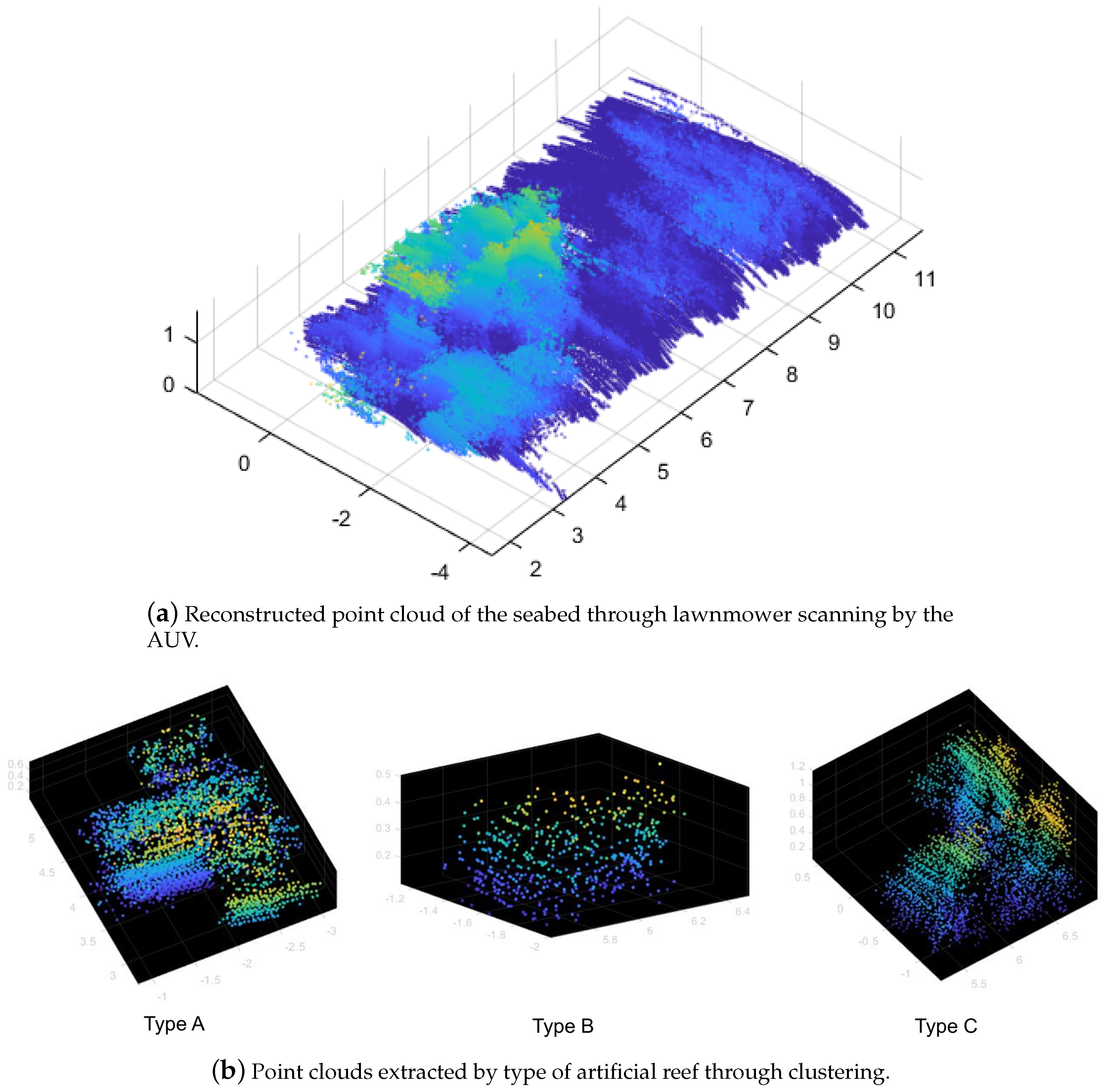
4.2. Field Experiment

For the testing of the proposed method, we also conducted a field experiment. The categories of objects that exist underwater are different from the types commonly found on land. Among underwater objects, we tested whether the proposed method could classify various types of artificial reefs through the field experiment.

4.2.1. Training of the Proposed Object Classifier

The NN of the proposed method was trained in advanced with a custom dataset consisting of point clouds of the artificial reefs. The training dataset can be constructed by installing target objects on the seabed, capturing sonar images through additional experiments, and generating point clouds of the objects with the proposed method. However, because the training requires a large amount of data, the experiments to acquire training data require considerable time and effort.

Instead, we could synthesize a point cloud for training in a short time using the proposed training data synthesis method, which modeled the target object in 3D using CAD and transformed the model to have the characteristics of a sonar-based point cloud. First, we modeled the 3D shapes of artificial reefs, as shown in Figure 12a. We made a rough 3D model of three typical artificial reefs of the East Sea in Korea with similar shapes and sizes using the photos and dimensions provided by the manufacturer [30]. Then, we assumed 72 scanning directions with the heading angle rotating around the object at 20-degree intervals and with the tilt angle changing from 20${}^{\circ }$ to 45${}^{\circ }$ for each model. As a result, base point clouds were generated by the proposed training data synthesis method, as shown in Figure 12b. The synthesized point clouds show characteristics such as the front slope and hidden surfaces according to the scan direction, which appear when reconstructing a point cloud by scanning a real object with a sonar sensor. To make the object classifier robust to the noise, we added 3D Gaussian noise points of 5% to 15% of the total number of points to these base point clouds. Finally, to normalize the point density and size of the point clouds as the input of the NN, 1024 points were randomly sampled and scaled to fit a unit sphere with a radius of one, as shown in Figure 12c. In total, 1296 point clouds were synthesized.

The NN of the proposed method was trained using these synthesized point clouds. Among 1296 point clouds, we used 1096 point clouds for the training of the NN and the remaining 200 point clouds for validation data. The NN was trained for 205 epochs. The training took about an hour using a single GPU Titan V.

4.2.2. Field Experiment Setup

Figure 13 illustrates the field experiment. An AUV equipped with an FSS was deployed into the sea of Jangil-bay, Pohang, Republic of Korea, as shown in Figure 13a,b. The AUV ‘Cyclops’ [31] was used as the AUV, and a dual-frequency identification sonar (DIDSON) [32] was used as the FSS; their specifications are described in

Table 1. Specifications of the AUV ’Cyclops’.

Features	Specifications
Dimension	0.9 m (width) × 1.5 m (length) × 0.9 m (height)
Weight	210 kg in air
Depth rating	100 m
Power source	600 Wh Li-Po battery × 2
Computing System	PC-104 (Intel Atom @ 1.66 GHz) × 2
Propulsion	8 thrusters (2 for surge, 4 for sway, 2 for heave)
Max speed	2 knots
Sensors	Forward-Scan Sonar (1.8 MHz)
	Doppler Velocity Logger (1.2 MHz)
	Digital pressure transducer
	Fiber-optic gyro

and

Table 2. Specifications of the DIDSON.

Features	Specifications
Operating frequency	1.8 MHz
Field of view	0.42–46.25 m (in range)
	−14.5–14.5${}^{\circ }$ (in azimuth)
	−7–7${}^{\circ }$ (in elevation)
Beam spreading angle	14${}^{\circ }$
Beam width	0.3${}^{\circ }$
Max resolution	0.3${}^{\circ }$
Image size	512 × 96
Frame rate	4–21 fps

, respectively. Through the investigation using the AUV, we found the seafloor in which three types of artificial reefs had been installed, as shown in Figure 13c. Four artificial reefs were found, with one type A, one type B, and two type Cs. As shown in Figure 13d, the AUV scanned the seabed near the sea area where the artificial reefs were installed with lawnmower trajectories. When the AUV moved in the lawnmower trajectory, it passed through the artificial reefs lying on the seabed in any direction, so the point clouds of the artificial reefs were generated. We checked whether the proposed method could classify various types of artificial reefs by generating point clouds during the AUV’s operation.

4.2.3. Field Experiment Results

As the AUV scanned the seafloor with the FSS while moving in a lawnmower trajectory, the proposed method first generated a 3D point cloud for the scanned area, as shown in Figure 14a. Then, the point clouds of the artificial reefs could be extracted through clustering, as shown in Figure 14b. Each point cloud consists of less than 3000 points. Managing these point clouds requires less memory than even a single 2D sonar image. Therefore, the proposed method could handle practical information about objects with small memory.

Then, we verified that the trained object classifier could distinguish the different types of underwater artificial reefs based on the generated point clouds. A total of 80 test point clouds were prepared by sampling 1024 points several times from all of the point clouds and applying rotation transformation to the point clouds. For a quick test, the inference of the trained classifier was also conducted using the GPU Titan V.

The precision and recall of the proposed method were also measured. The proposed method recorded 92.3% precision and 90.0% recall. To compare the accuracy of the proposed method, we built a convolutional neural network (CNN) for object recognition based on a single 2D image [33]. We trained the CNN using a simulated 2D sonar image of the target object; however, the CNN failed to recognized objects given real sonar images captured in the field because there were differences of illumination and characteristics of noises between simulated and real sonar images. On the other hand, the proposed method, which was also trained using the synthesized training dataset, could classify the objects. There were differences between the synthesized training point clouds and the point clouds reconstructed from actual artificial reefs because we approximated the artificial reefs in the 3D model and because bio-fouling occurred in the artificial reefs. Furthermore, as shown in type A of Figure 14b, part of the artificial reef was not correctly reconstructed due to occlusion. Nevertheless, the proposed method could classify the actual artificial reefs on the seabed. Because it is challenging to obtain base data for training in an underwater environment, that it can classify objects using synthesized training data by modeling the rough 3D shape of the target object is an advantage of the proposed method.

5. Conclusions

This paper proposes an underwater object classification method for an AUV that reconstructs an object into a 3D point cloud and predicts the class with an NN. The AUV could capture sonar images during its mission and generate a point cloud of an underwater scene by analyzing the highlights of the sonar image. Then, object point cloud candidates were obtained through clustering and removal. Finally, the NN could classify the underwater objects by predicting the labels of the point clouds.

By restoring the 3D geometry of the object, the proposed method could classify the object accurately utilizing the lost information, and it also simplified the training process. Furthermore, the restoration of 3D geometry is made in a point cloud format through a single scan by an AUV, so it requires less memory and time and is suitable for use by the AUV. Finally, the introduction of an NN facilitated robust classification, even when using a low-resolution and noisy sonar sensor.

An AUV can construct a 3D map for an underwater scene and recognize objects in the map using the proposed method. This information is expected to be applicable to various AUV operations, such as terrain-based navigation and target object detection. Furthermore, because a point cloud is a data format often used as an input to various terrestrial robot algorithms, the proposed method can improve the utilization of the underwater sonar data.

References

1. Kim, T.; Kim, J.; Byun, S.W. A comparison of nonlinear filter algorithms for terrain-referenced underwater navigation. Int. J. Control Autom. Syst. 2018, 16, 2977–2989. [Google Scholar] [CrossRef]
2. Lee, D.; Kim, G.; Kim, D.; Myung, H.; Choi, H.T. Vision-based object detection and tracking for autonomous navigation of underwater robots. Ocean Eng. 2012, 48, 59–68. [Google Scholar] [CrossRef]
3. Tang, Z.; Wang, Z.; Lu, J.; Ma, G.; Zhang, P. Underwater robot detection system based on fish’s lateral line. Electronics 2019, 8, 566. [Google Scholar] [CrossRef] [Green Version]
4. Johannsson, H.; Kaess, M.; Englot, B.; Hover, F.; Leonard, J. Imaging sonar-aided navigation for autonomous underwater harbor surveillance. In Proceedings of the 2010 IEEE/RSJ International Conference on Intelligent Robots and Systems, Taipei, Taiwan, 18–22 October 2010; pp. 4396–4403. [Google Scholar]
5. Bingham, B.; Foley, B.; Singh, H.; Camilli, R.; Delaporta, K.; Eustice, R.; Mallios, A.; Mindell, D.; Roman, C.; Sakellariou, D. Robotic tools for deep water archaeology: Surveying an ancient shipwreck with an autonomous underwater vehicle. J. Field Robot. 2010, 27, 702–717. [Google Scholar] [CrossRef] [Green Version]
6. Stokey, R.P.; Roup, A.; von Alt, C.; Allen, B.; Forrester, N.; Austin, T.; Goldsborough, R.; Purcell, M.; Jaffre, F.; Packard, G.; et al. Development of the REMUS 600 autonomous underwater vehicle. In Proceedings of the OCEANS 2005 MTS/IEEE, Washington, DC, USA, 17–23 September 2005; pp. 1301–1304. [Google Scholar]
7. Nakatani, T.; Ura, T.; Ito, Y.; Kojima, J.; Tamura, K.; Sakamaki, T.; Nose, Y. AUV “TUNA-SAND” and its Exploration of hydrothermal vents at Kagoshima Bay. In Proceedings of the OCEANS 2008-MTS/IEEE Kobe Techno-Ocean, Kobe, Japan, 8–11 April 2008; pp. 1–5. [Google Scholar]
8. Reed, S.; Petillot, Y.; Bell, J. An automatic approach to the detection and extraction of mine features in sidescan sonar. IEEE J. Ocean Eng. 2003, 28, 90–105. [Google Scholar] [CrossRef]
9. Kim, B.; Yu, S.C. Imaging sonar based real-time underwater object detection utilizing adaboost method. In Proceedings of the 2017 IEEE Underwater Technology (UT), Busan, Korea, 21–24 February 2017; pp. 1–5. [Google Scholar]
10. Karimanzira, D.; Renkewitz, H.; Shea, D.; Albiez, J. Object Detection in Sonar Images. Electronics 2020, 9, 1180. [Google Scholar] [CrossRef]
11. Maki, T.; Horimoto, H.; Ishihara, T.; Kofuji, K. Tracking a Sea Turtle by an AUV with a Multibeam Imaging Sonar: Toward Robotic Observation of Marine Life. Int. J. Control Autom. Syst. 2020, 18, 597–604. [Google Scholar] [CrossRef]
12. Kim, J.; Kim, T.; Kim, J.; Rho, S.; Song, Y.w.; Yu, S.C. Simulation and Feasibility Test of Mini-ROVs with AUV for the Manipulation Purpose. In Proceedings of the OCEANS 2019 MTS/IEEE SEATTLE, Seattle, WA, USA, 27–31 October 2019; pp. 1–6. [Google Scholar]
13. Lee, S.; Park, B.; Kim, A. Deep learning from shallow dives: Sonar image generation and training for underwater object detection. arXiv 2018, arXiv:1810.07990. [Google Scholar]
14. Myers, V.; Williams, D.P. Adaptive multiview target classification in synthetic aperture sonar images using a partially observable Markov decision process. IEEE J. Ocean Eng. 2011, 37, 45–55. [Google Scholar] [CrossRef]
15. Cho, H.; Gu, J.; Yu, S.C. Robust sonar-based underwater object recognition against angle-of-view variation. IEEE Sens. J. 2015, 16, 1013–1025. [Google Scholar] [CrossRef]
16. Lee, M.; Kim, J.; Yu, S.C. Robust 3D Shape Classification Method using Simulated Multi View Sonar Images and Convolutional Nueral Network. In Proceedings of the OCEANS 2019-Marseille, Marseille, France, 17–20 June 2019; pp. 1–5. [Google Scholar]
17. Das, J.; Rajany, K.; Frolovy, S.; Pyy, F.; Ryany, J.; Caronz, D.A.; Sukhatme, G.S. Towards marine bloom trajectory prediction for AUV mission planning. In Proceedings of the 2010 IEEE International Conference on Robotics and Automation, Anchorage, AK, USA, 3–7 May 2010; pp. 4784–4790. [Google Scholar]
18. Cho, H.; Kim, B.; Yu, S.C. AUV-based underwater 3-D point cloud generation using acoustic lens-based multibeam sonar. IEEE J. Ocean Eng. 2017, 43, 856–872. [Google Scholar] [CrossRef]
19. Ester, M.; Kriegel, H.P.; Sander, J.; Xu, X. A density-based algorithm for discovering clusters in large spatial databases with noise. In Proceedings of the Knowledge Discovery and Data Mining, Portland, OR, USA, 2–4 August 1996; Volume 96, pp. 226–231. [Google Scholar]
20. Cho, Y.; Jang, H.; Malav, R.; Pandey, G.; Kim, A. Underwater Image Dehazing via Unpaired Image-to-image Translation. Int. J. Control Autom. Syst. 2020, 18, 605–614. [Google Scholar] [CrossRef]
21. Wang, W.; Yu, R.; Huang, Q.; Neumann, U. Sgpn: Similarity group proposal network for 3d point cloud instance segmentation. In Proceedings of the IEEE Conference on Computer Vision and Pattern Recognition, Salt Lake City, UT, USA, 18–22 June 2018; pp. 2569–2578. [Google Scholar]
22. Qi, C.R.; Su, H.; Mo, K.; Guibas, L.J. Pointnet: Deep learning on point sets for 3d classification and segmentation. In Proceedings of the IEEE Conference on Computer Vision and Pattern Recognition, Honolulu, HI, USA, 21–26 July 2017; pp. 652–660. [Google Scholar]
23. Joe, H.; Kim, J.; Yu, S.C. 3D Reconstruction Using Two Sonar Devices in a Monte-Carlo Approach for AUV Application. Int. J. Control Autom. Syst. 2020, 18, 587–596. [Google Scholar] [CrossRef]
24. Wu, Z.; Song, S.; Khosla, A.; Yu, F.; Zhang, L.; Tang, X.; Xiao, J. 3d shapenets: A deep representation for volumetric shapes. In Proceedings of the IEEE Conference on Computer Vision and Pattern Recognition, Boston, MA, USA, 7–12 June 2015; pp. 1912–1920. [Google Scholar]
25. Manhães, M.M.M.; Scherer, S.A.; Voss, M.; Douat, L.R.; Rauschenbach, T. UUV simulator: A gazebo-based package for underwater intervention and multi-robot simulation. In Proceedings of the OCEANS 2016 MTS/IEEE Monterey, Monterey, CA, USA, 19–23 September 2016; pp. 1–8. [Google Scholar]
26. Cieślak, P. Stonefish: An Advanced Open-Source Simulation Tool Designed for Marine Robotics, with a ROS Interface. In Proceedings of the OCEANS 2019-Marseille, Marseille, France, 17–20 June 2019; pp. 1–6. [Google Scholar]
27. Kim, J.; Sung, M.; Yu, S.C. Development of Simulator for Autonomous Underwater Vehicles utilizing Underwater Acoustic and Optical Sensing Emulators. In Proceedings of the 2018 18th International Conference on Control, Automation and Systems (ICCAS), Daegwallyeong, Korea, 17–20 October 2018; pp. 416–419. [Google Scholar]
28. Catmull, E. A Subdivision Algorithm for Computer Display of Curved Surfaces; Technical Report; Utah Univ. Salt Lake City School Of Computing: Salt Lake City, UT, USA, 1974. [Google Scholar]
29. Perreault, C.; Auclair-Fortier, M.F. Speckle simulation based on B-mode echographic image acquisition model. In Proceedings of the Fourth Canadian Conference on Computer and Robot Vision (CRV’07), Montreal, QC, Canada, 28–30 May 2007; pp. 379–386. [Google Scholar]
30. Sin, H. Artificial Reef Information Book. 2020. Available online: https://www.fira.or.kr/fira/fira_040301.jsp?mode=view&article_no=26351 (accessed on 22 October 2020).
31. Pyo, J.; Cho, H.; Joe, H.; Ura, T.; Yu, S.C. Development of hovering type AUV “Cyclops” and its performance evaluation using image mosaicing. Ocean Eng. 2015, 109, 517–530. [Google Scholar] [CrossRef] [Green Version]
32. Belcher, E.; Hanot, W.; Burch, J. Dual-frequency identification sonar (DIDSON). In Proceedings of the 2002 Interntional Symposium on Underwater Technology (Cat. No. 02EX556), Tokyo, Japan, 19 April 2002; pp. 187–192. [Google Scholar]
33. Redmon, J.; Divvala, S.; Girshick, R.; Farhadi, A. You only look once: Unified, real-time object detection. In Proceedings of the IEEE Conference on Computer Vision and Pattern Recognition, Las Vegas, NV, USA, 27–30 June 2016; pp. 779–788. [Google Scholar]
Figure 1. Imaging mechanism of the FSS.
Electronics 09 01763 g001
Figure 2. Difficulties in object classification using a 2D sonar image.
Electronics 09 01763 g002
Figure 3. Pipeline of the proposed underwater object classification method.
Electronics 09 01763 g003
Figure 4. Elevation angle restoration using the highlight extension effect as the FSS approaches an object.
Electronics 09 01763 g004
Figure 5. Calculation of an object’s coordinates using the highlight extension.
Electronics 09 01763 g005
Figure 6. Architecture of the neural network (NN) in the proposed method. The number in parentheses means the number of nodes in the layer.
Electronics 09 01763 g006
Figure 7. Front slope of the generated point cloud.
Electronics 09 01763 g007
Figure 8. Modeling of the front slope using navigational data of the autonomous underwater vehicle (AUV).
Electronics 09 01763 g008
Figure 9. Hidden surface removal by analyzing the scan line of the FSS.
Electronics 09 01763 g009
Figure 10. Design of the simulation experiment to verify the object classification using the sonar-based point cloud generation.
Electronics 09 01763 g010
Figure 11. Point cloud generation results of the simulation. (a) Objects modeled in 3D. (b) Synthesized sonar images while moving the FSS. (c) Generated point clouds of the objects.
Electronics 09 01763 g011
Figure 12. Synthesizing training point clouds from 3D-modeled objects (artificial reefs). (a) Rough 3D models of the artificial reefs. (b) Point clouds synthesized from the 3D models. (c) Normalized and noise-added point clouds for training.
Electronics 09 01763 g012
Figure 13. Field experiment for the artificial reef classification.
Electronics 09 01763 g013
Figure 14. Point clouds of artificial reefs generated in field experiments.
Electronics 09 01763 g014