Performance Analysis of Sparse Matrix-Vector Multiplication (SpMV) on Graphics Processing Units (GPUs)


Abstract
1. Introduction
2. Dataset, Sparsity Features, and Performance Metrics
2.1. Dataset and Sparsity Features
2.2. Performance Metrics
3. Compressed Sparse Row (CSR)
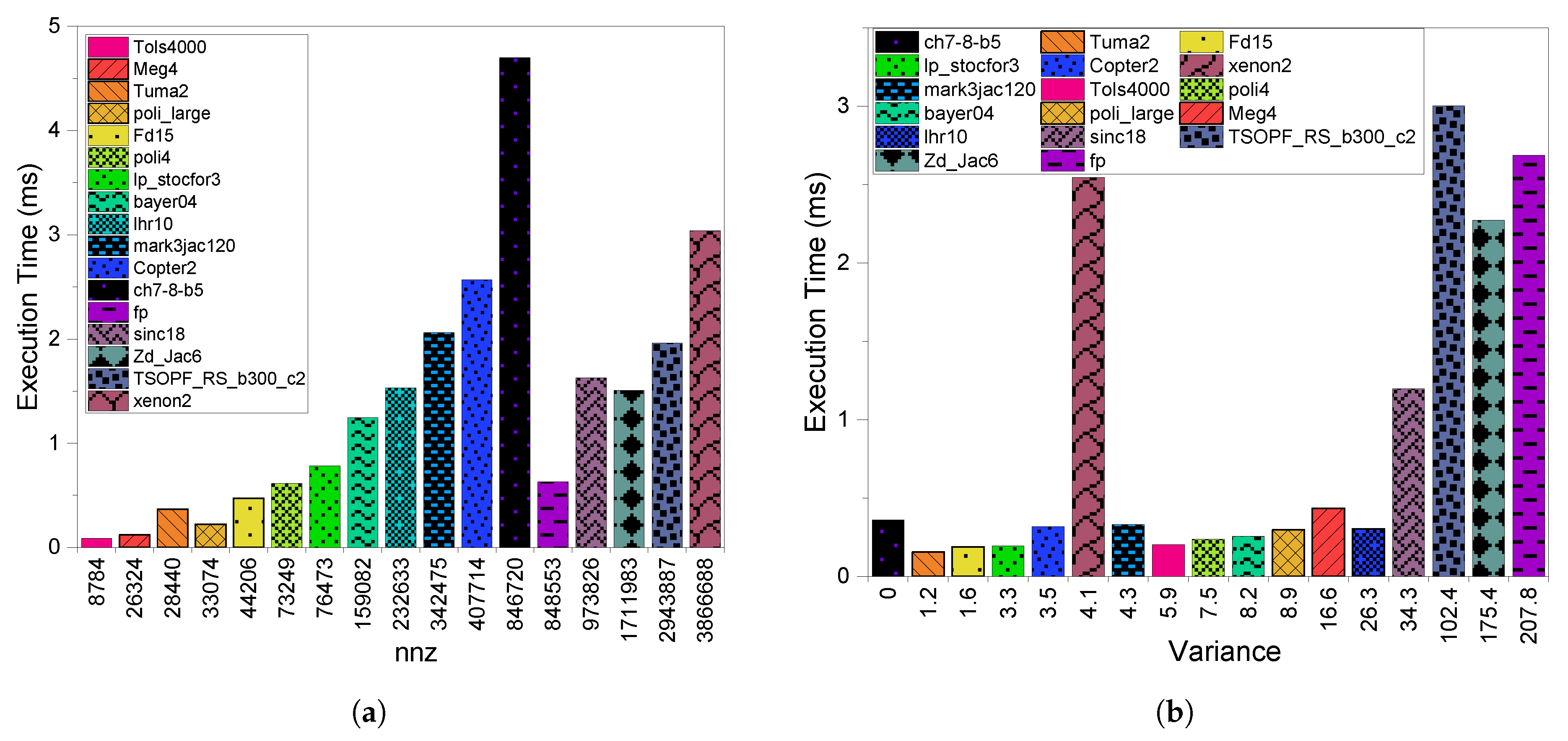
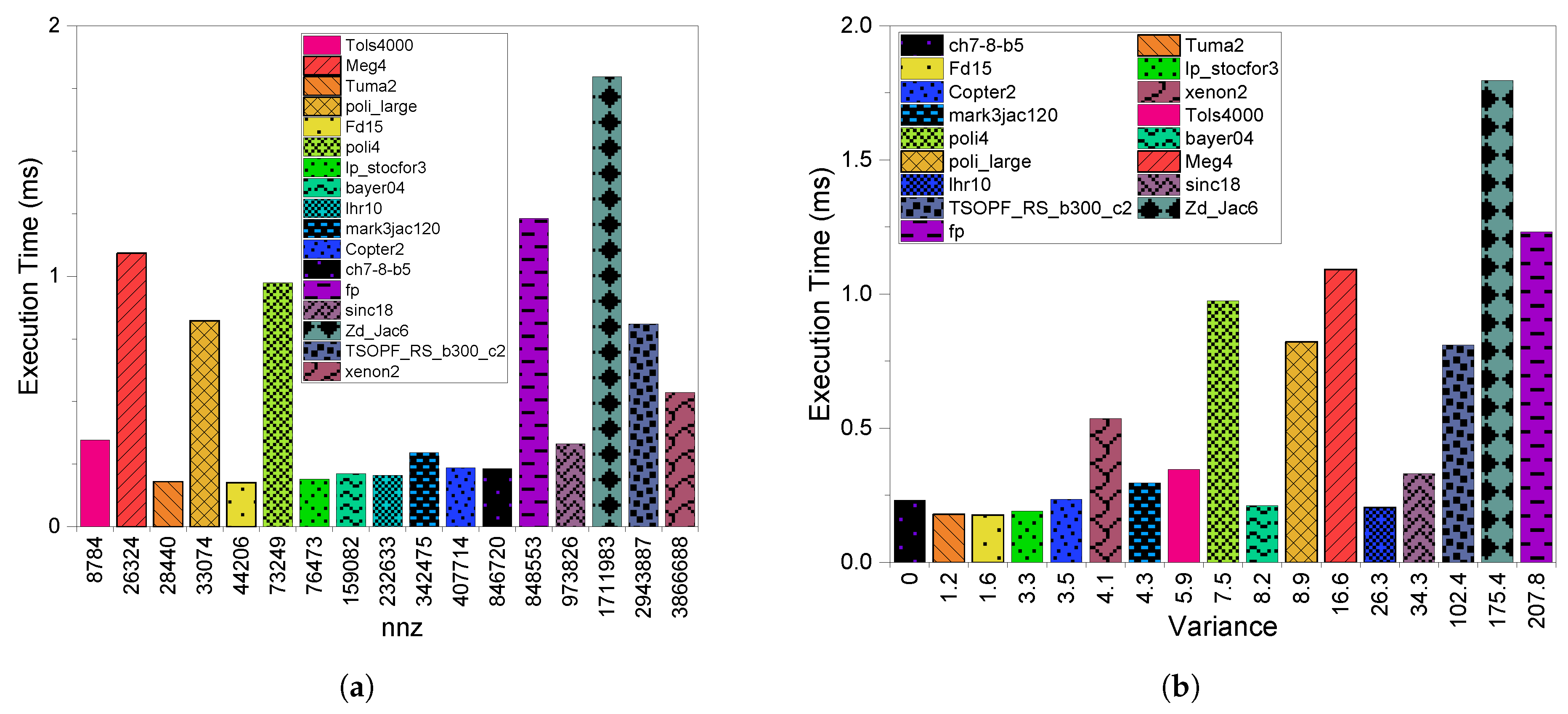
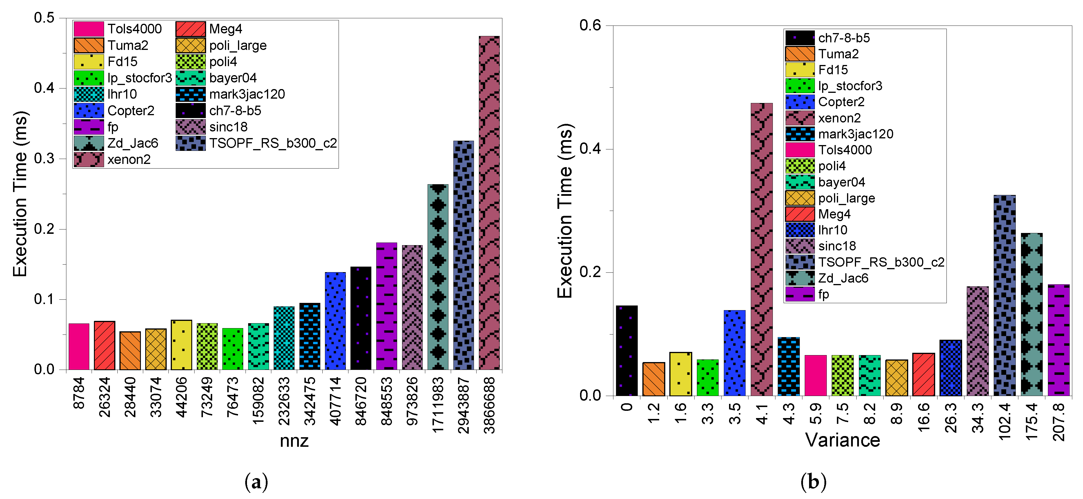
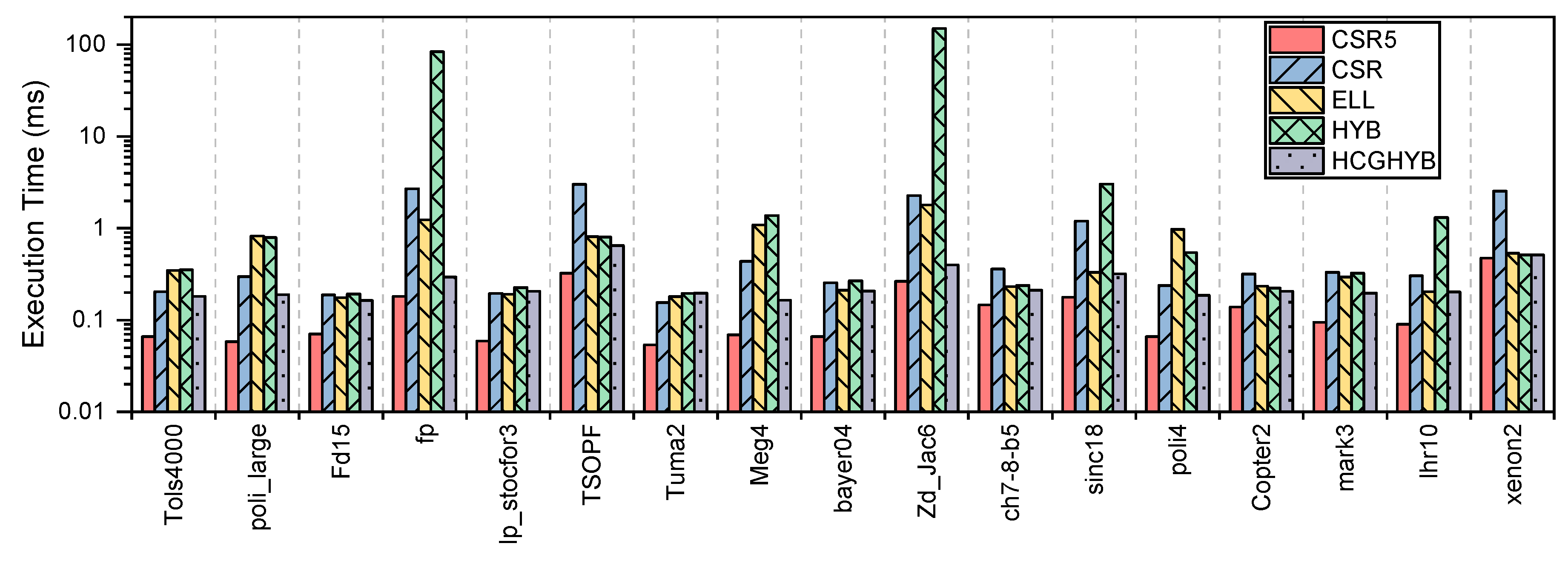
3.1. Execution Time
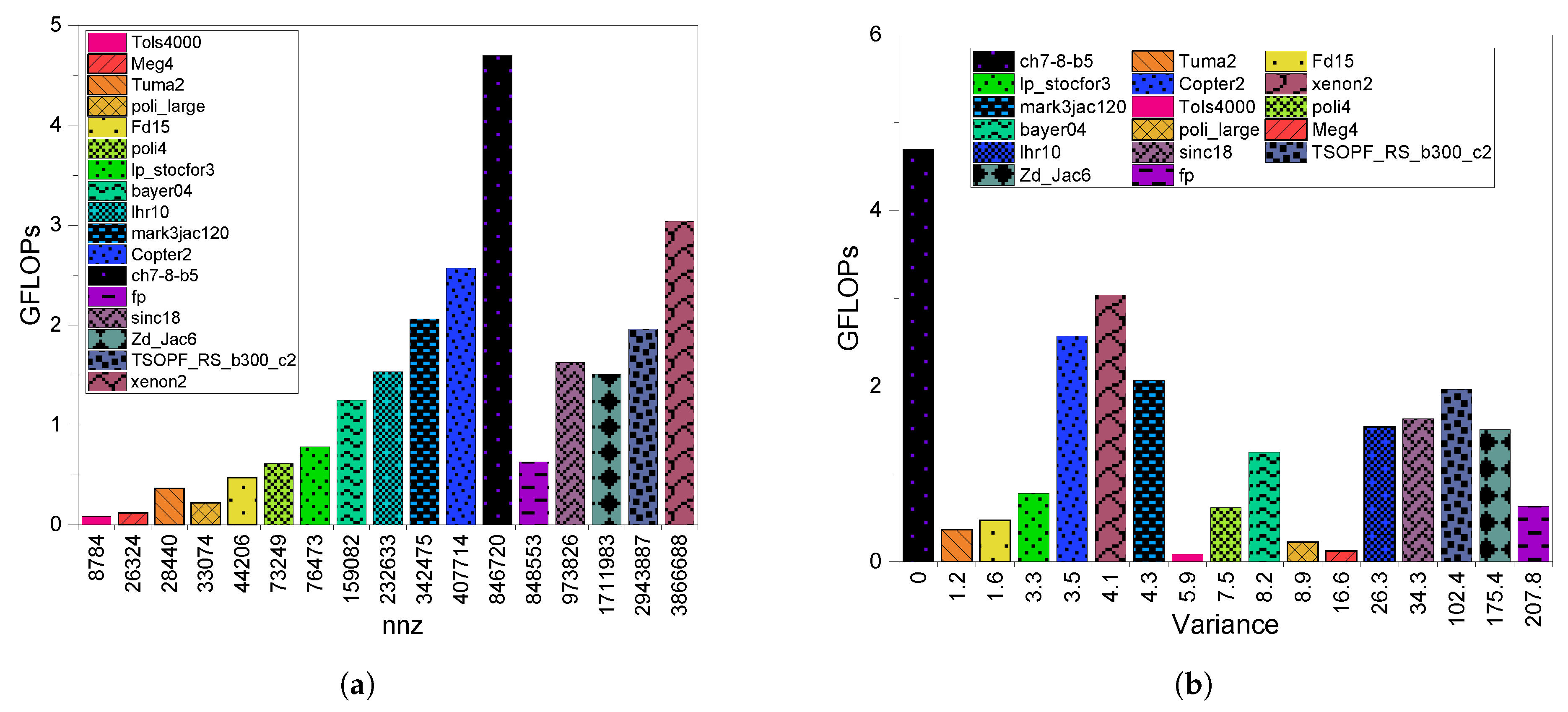
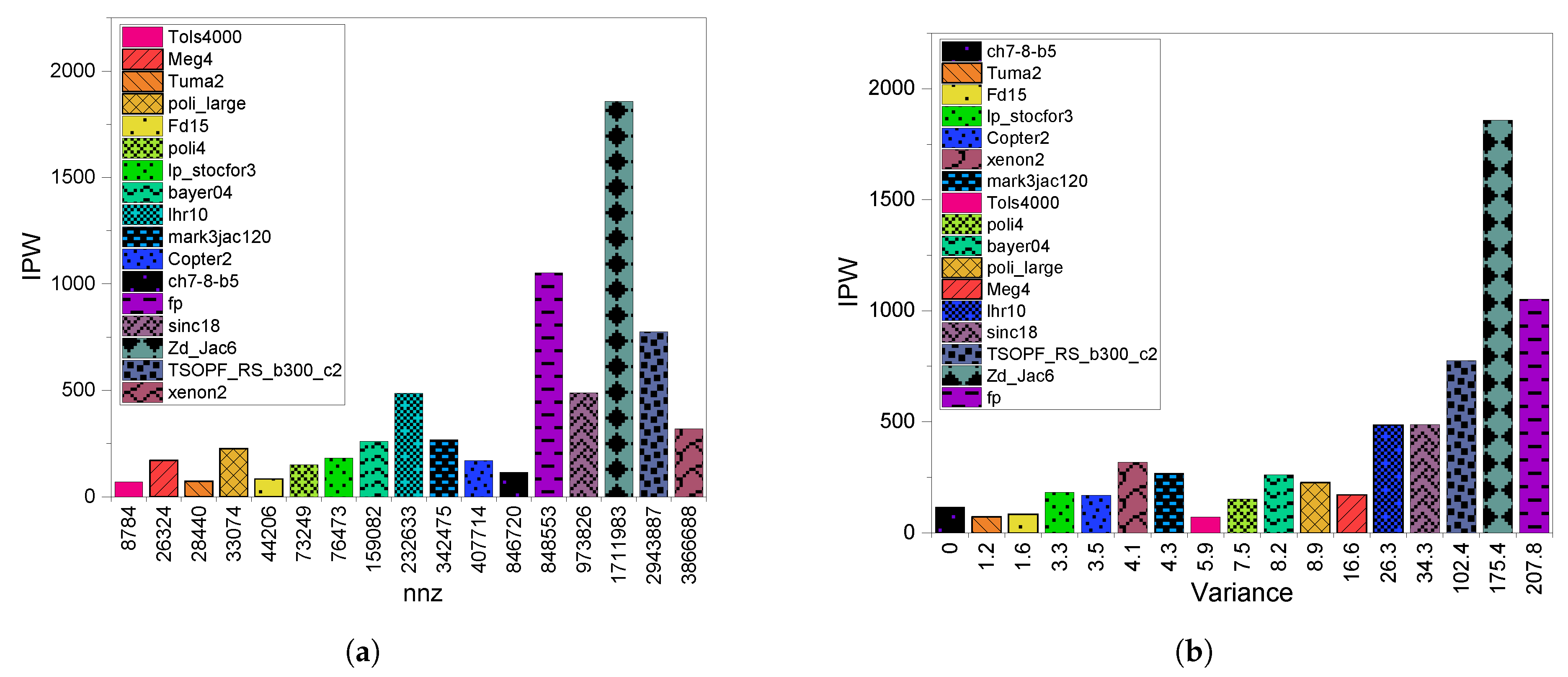
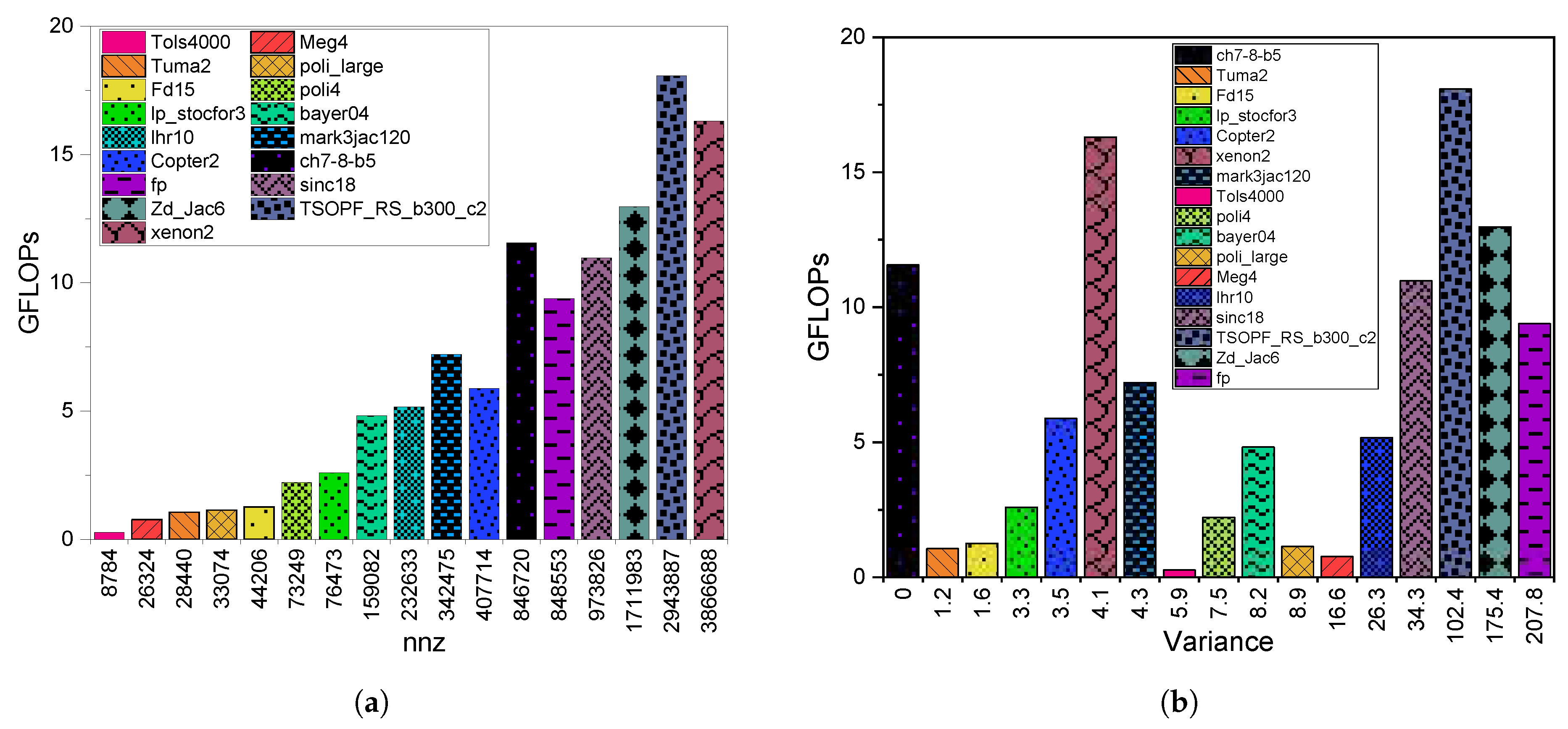
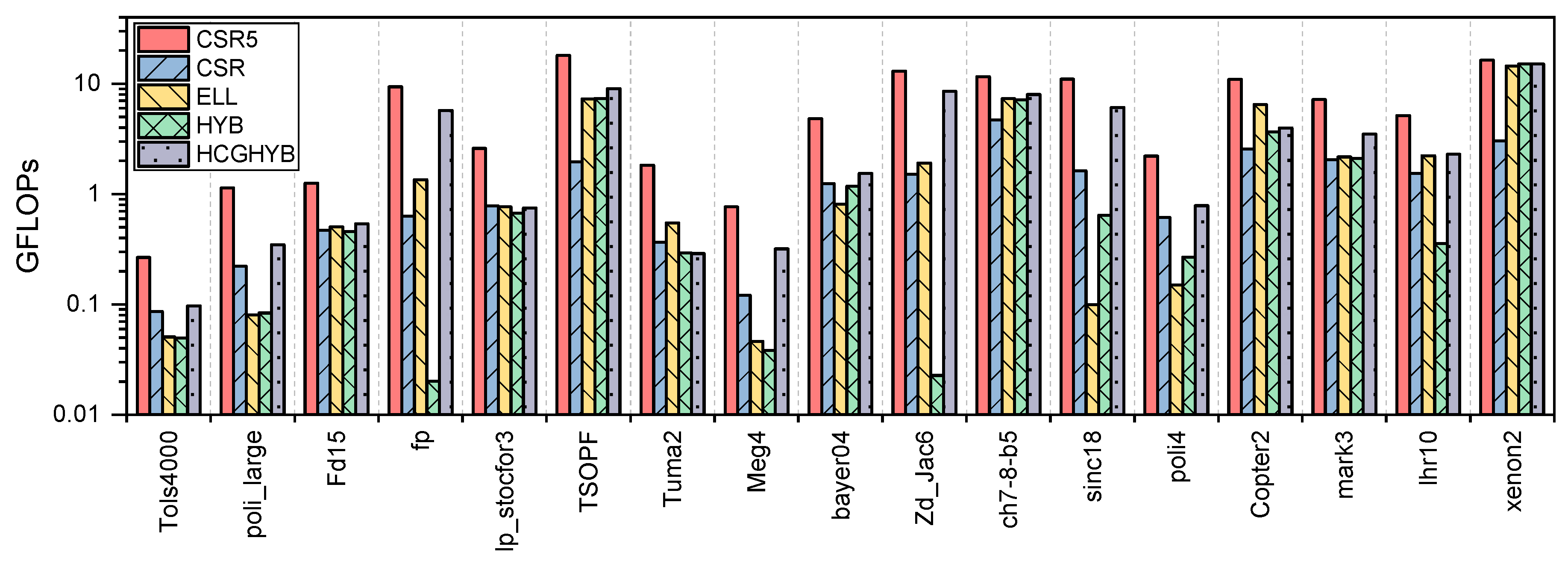
3.2. GPU Throughput
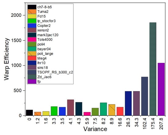
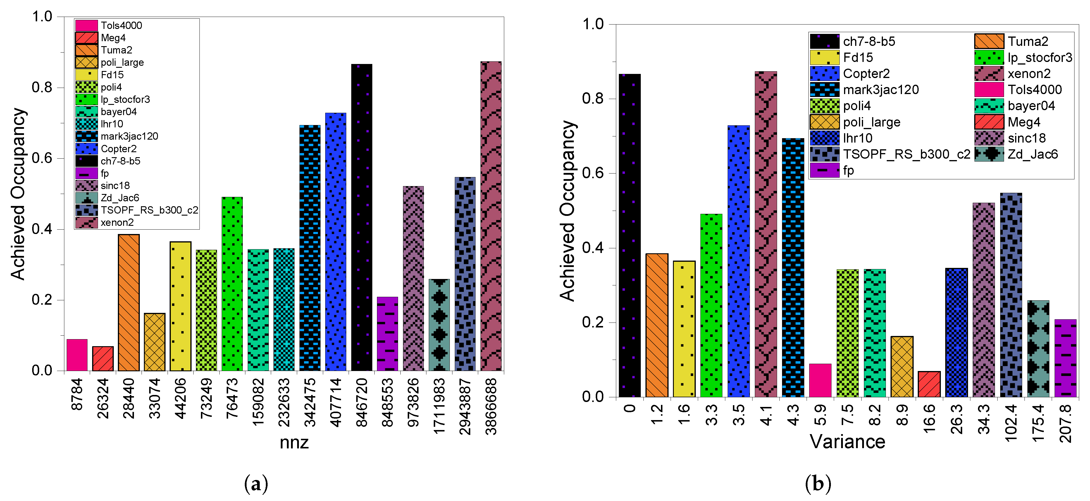
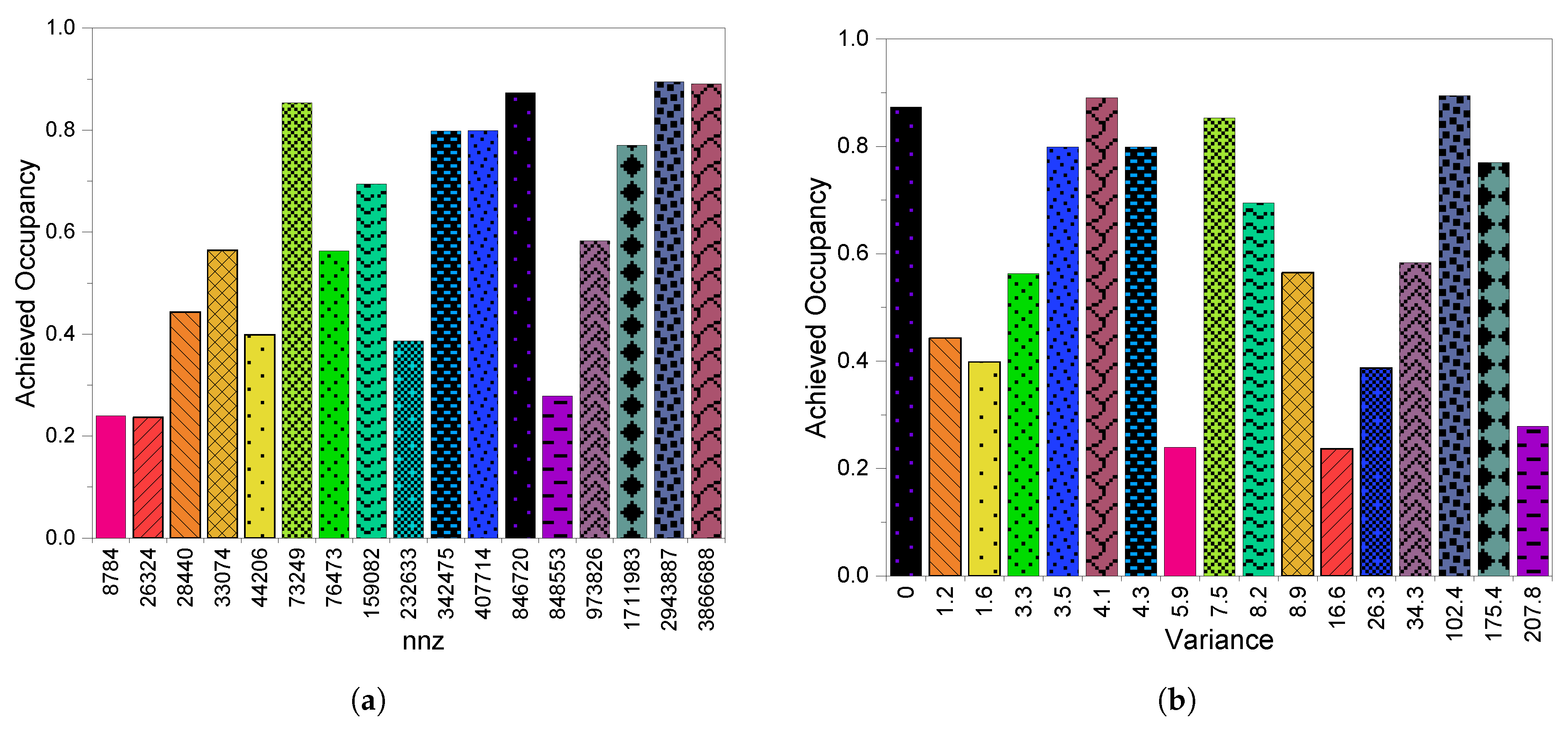
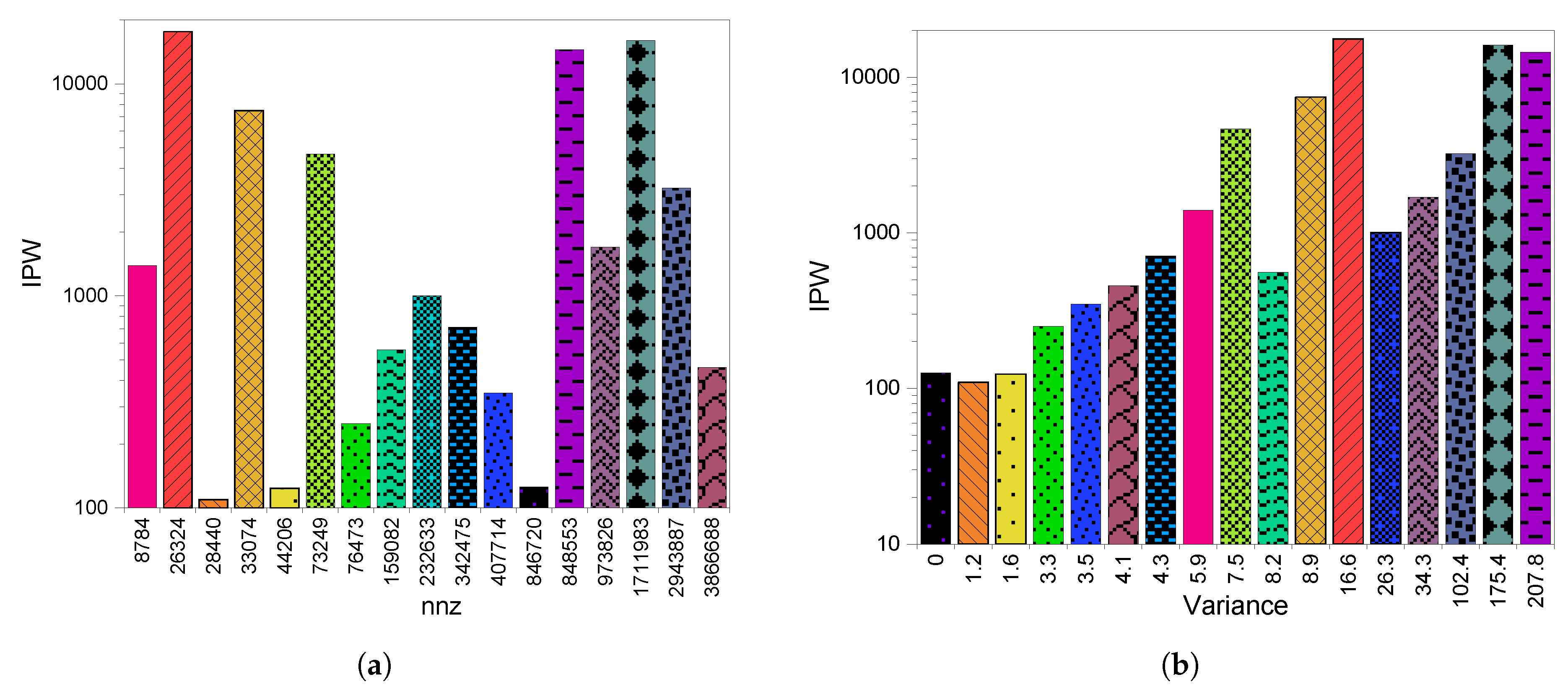
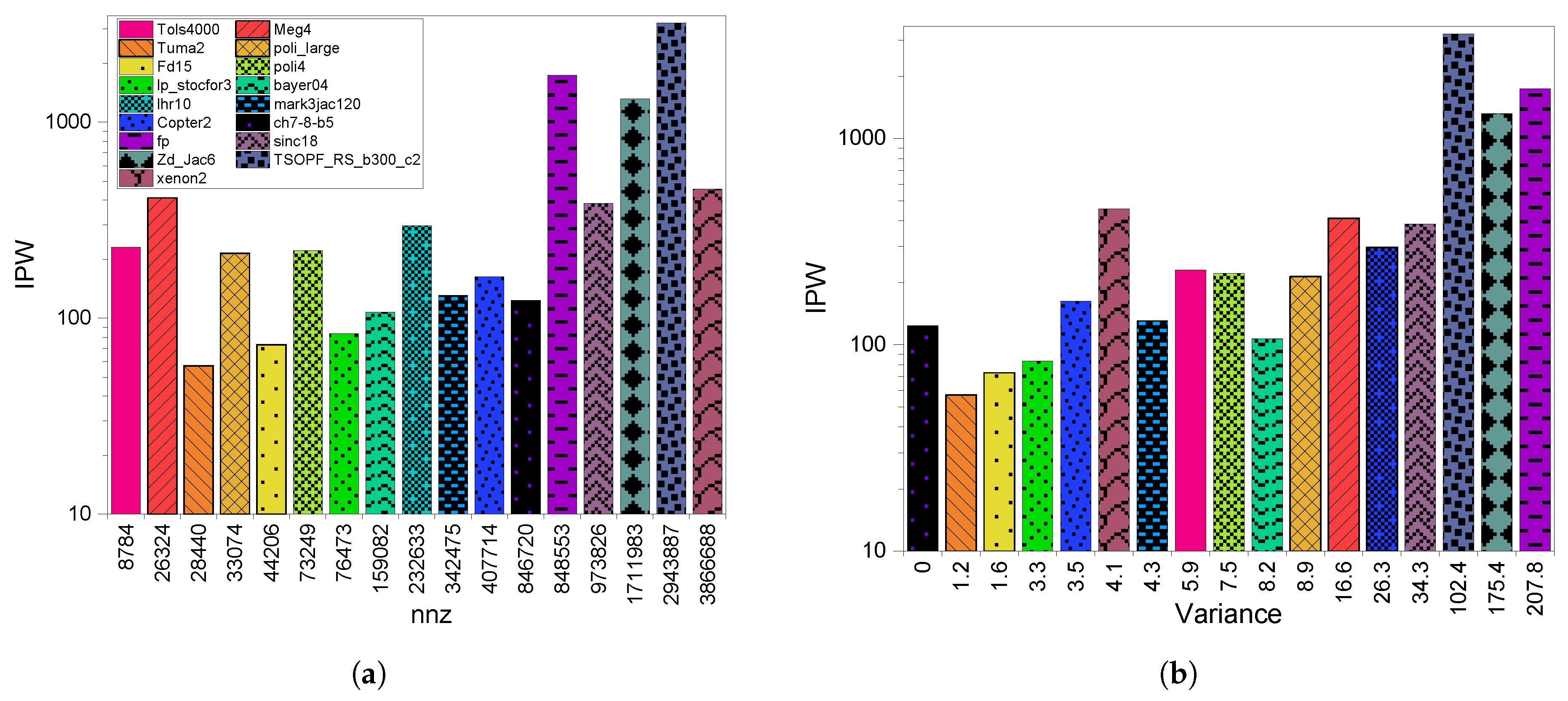
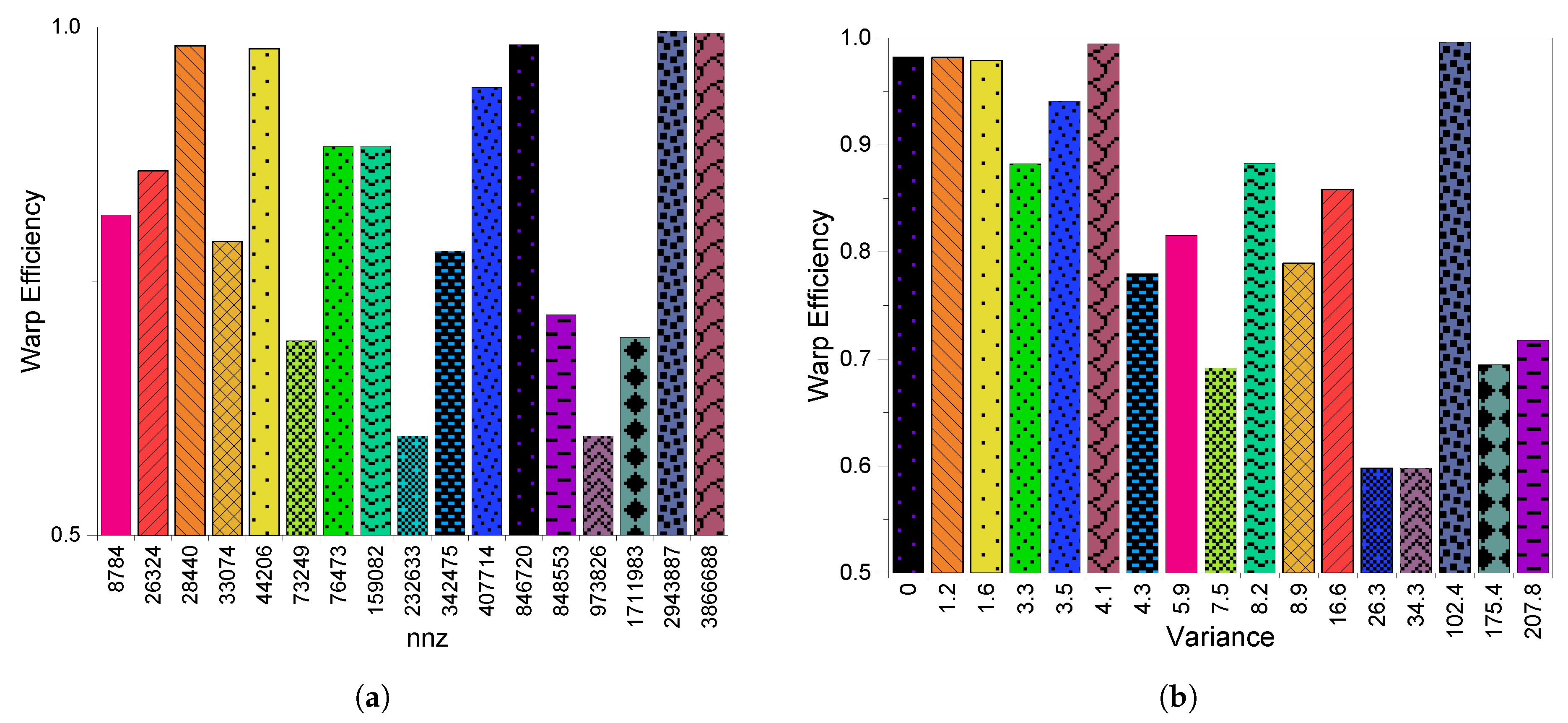
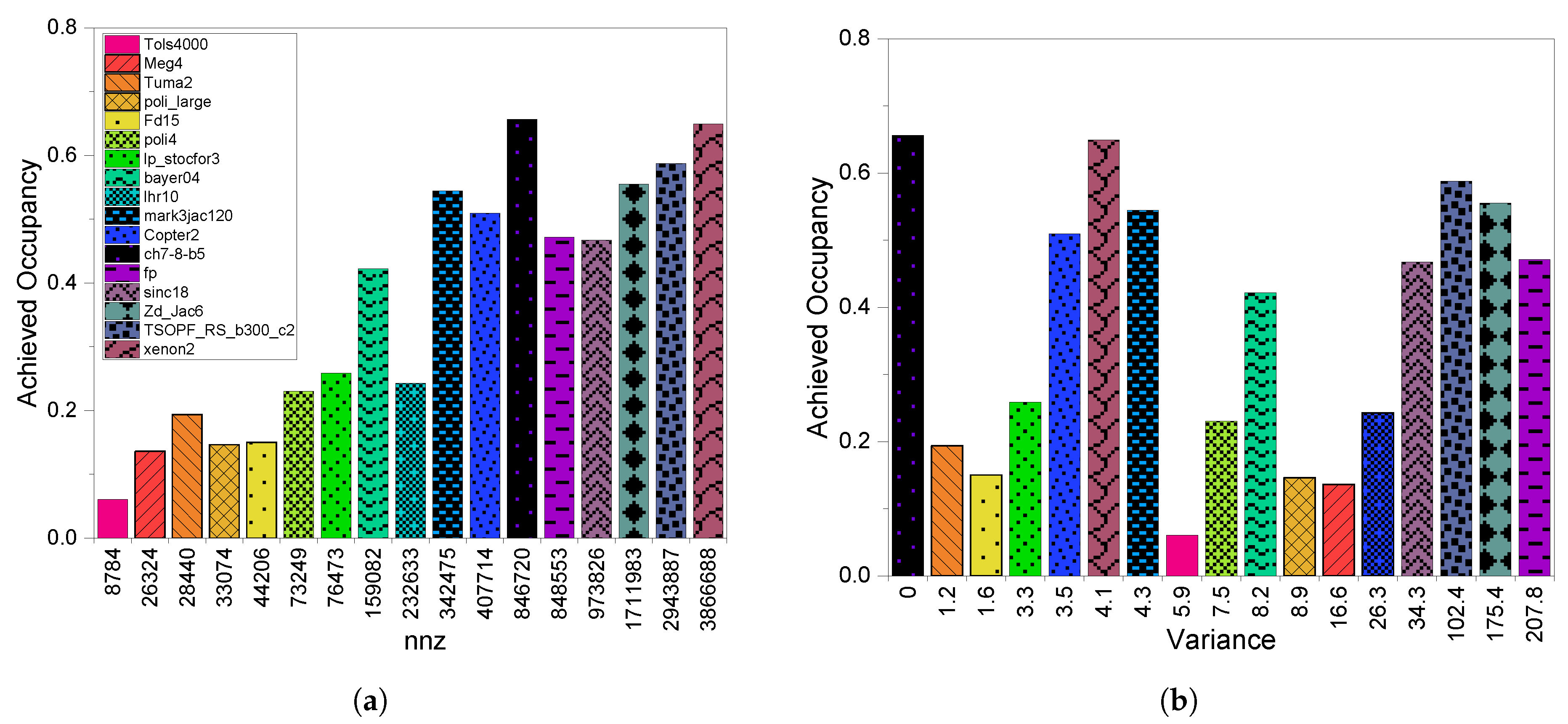
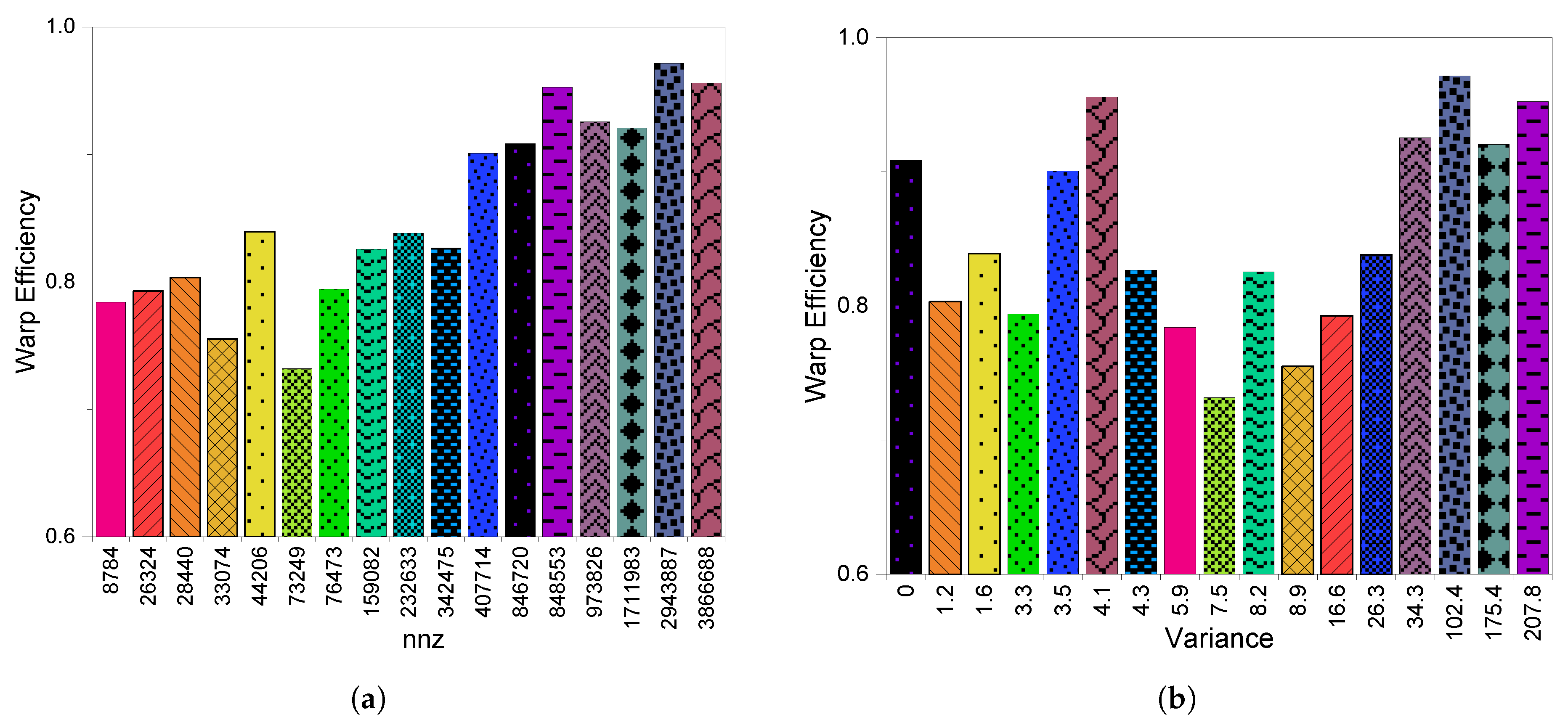
3.3. GPU Utilization
4. ELLPACK (ELL)
4.1. Execution Time
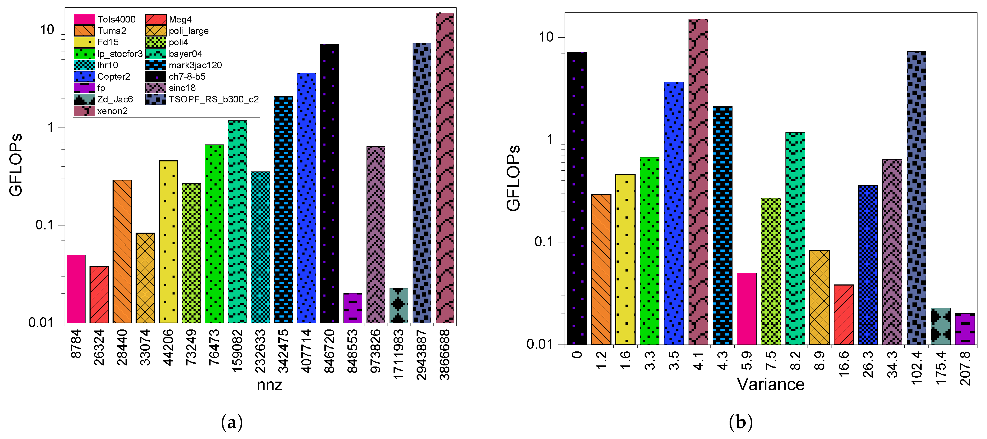
4.2. GPU Throughput
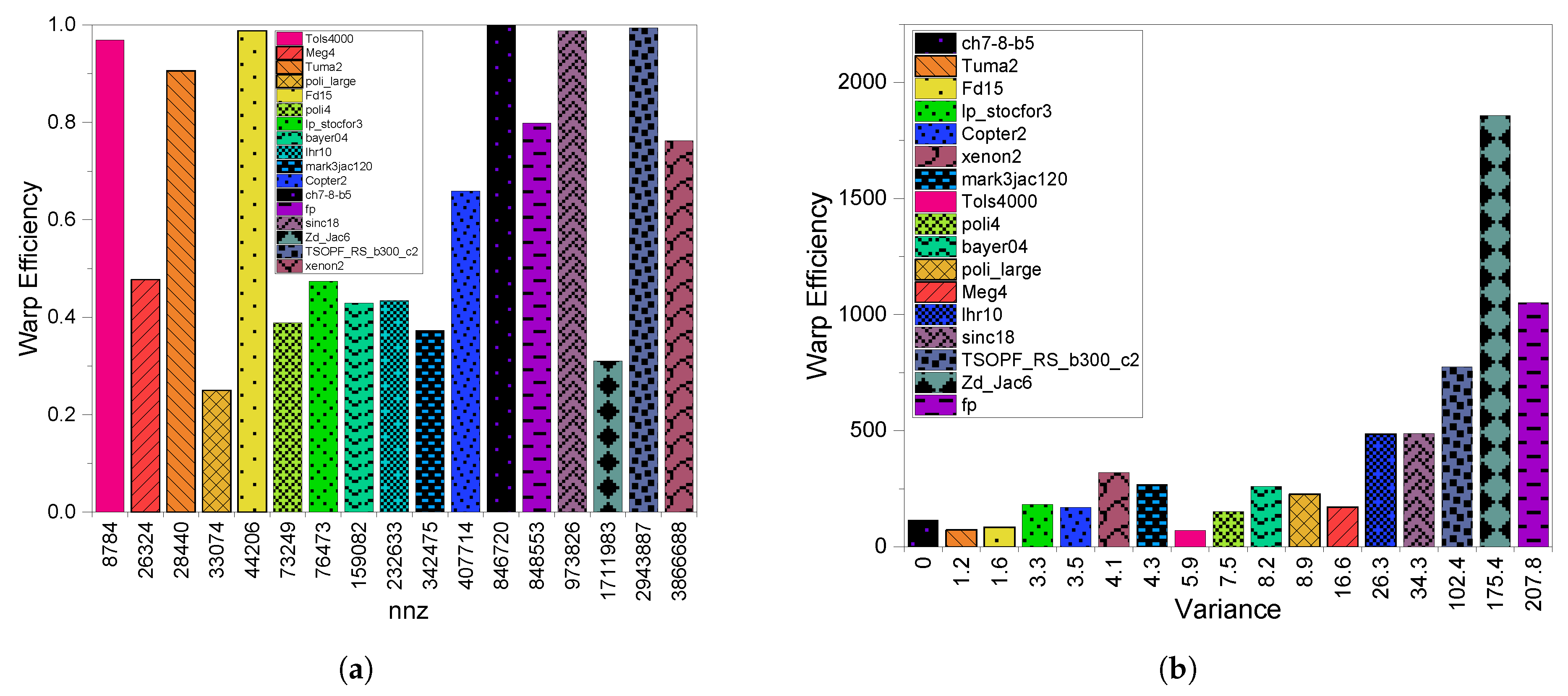
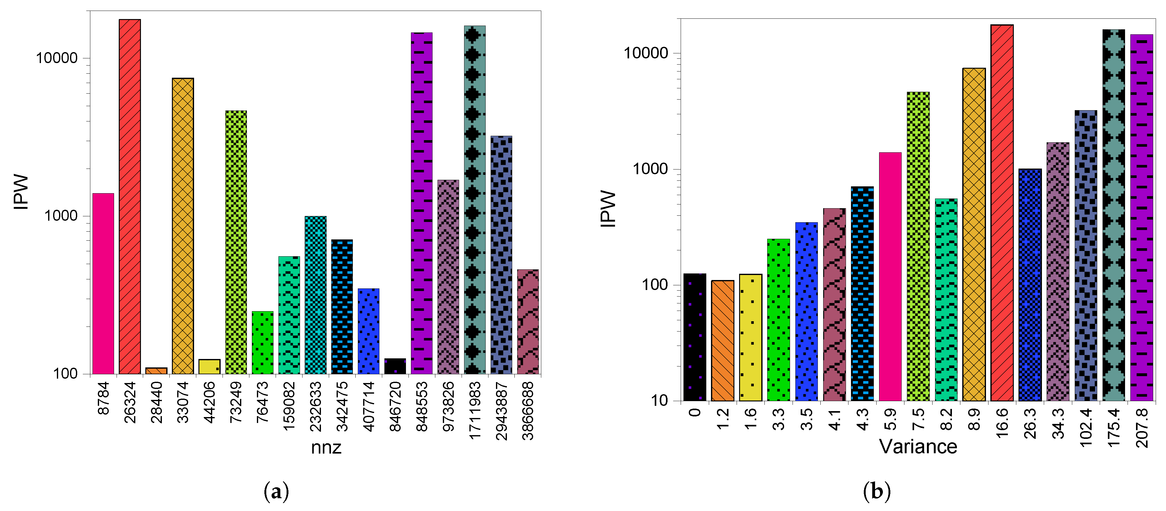
4.3. GPU Utilization
5. Hybrid ELL/COO (HYB)
5.1. Execution Time
5.2. GPU Throughput
5.3. GPU Utilization
6. Compressed Sparse Row 5 (CSR5)
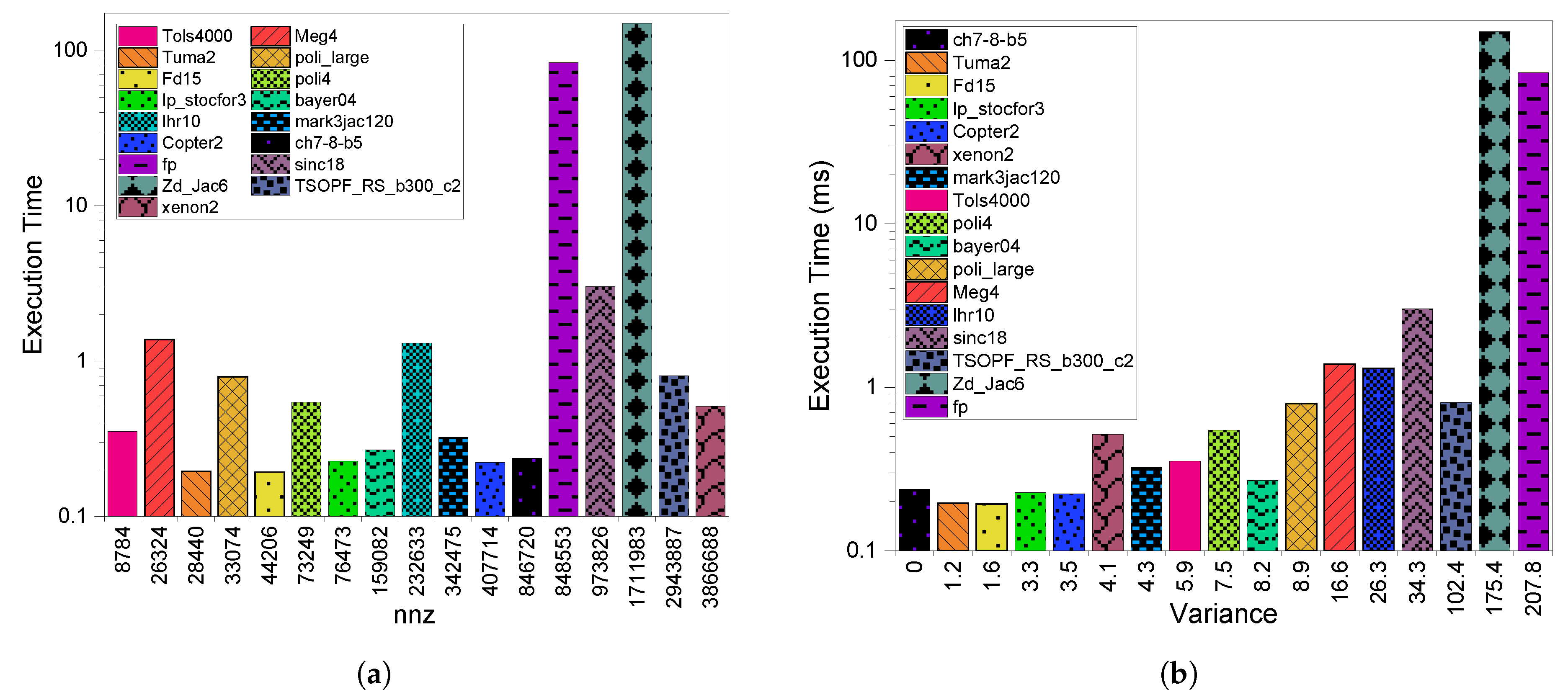
6.1. Execution Time
6.2. GPU Throughput
6.3. GPU Utilization
7. SpMV Performance on GPUs (Summary)
8. The Proposed Scheme (HCGHYB)
8.1. HCGHYB: Motivation and Description
8.2. HCGHYB: Performance Analysis
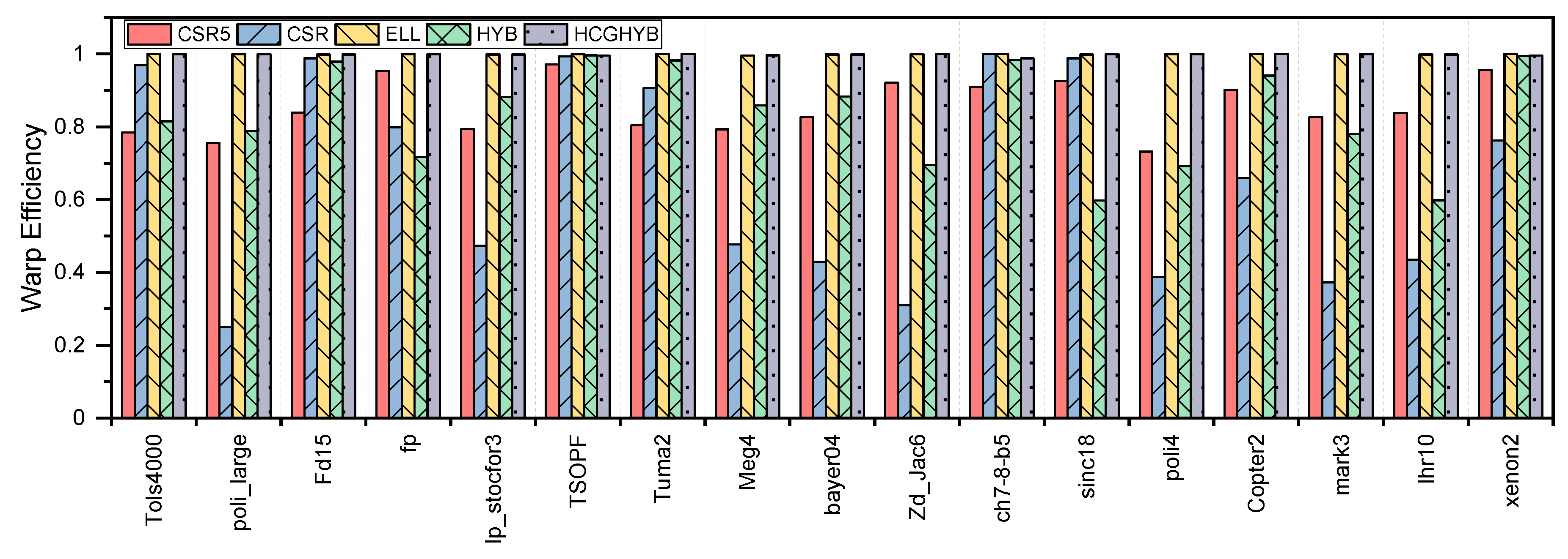
8.2.1. Execution Time
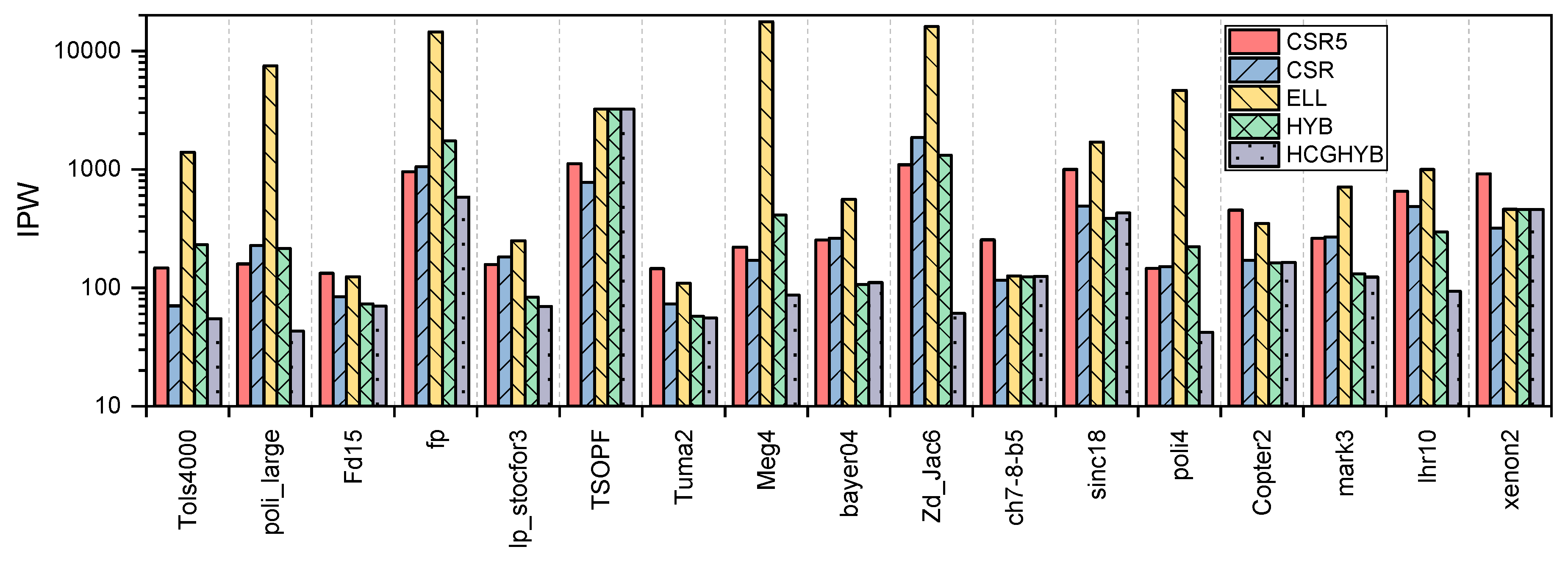
8.2.2. GPU Throughput
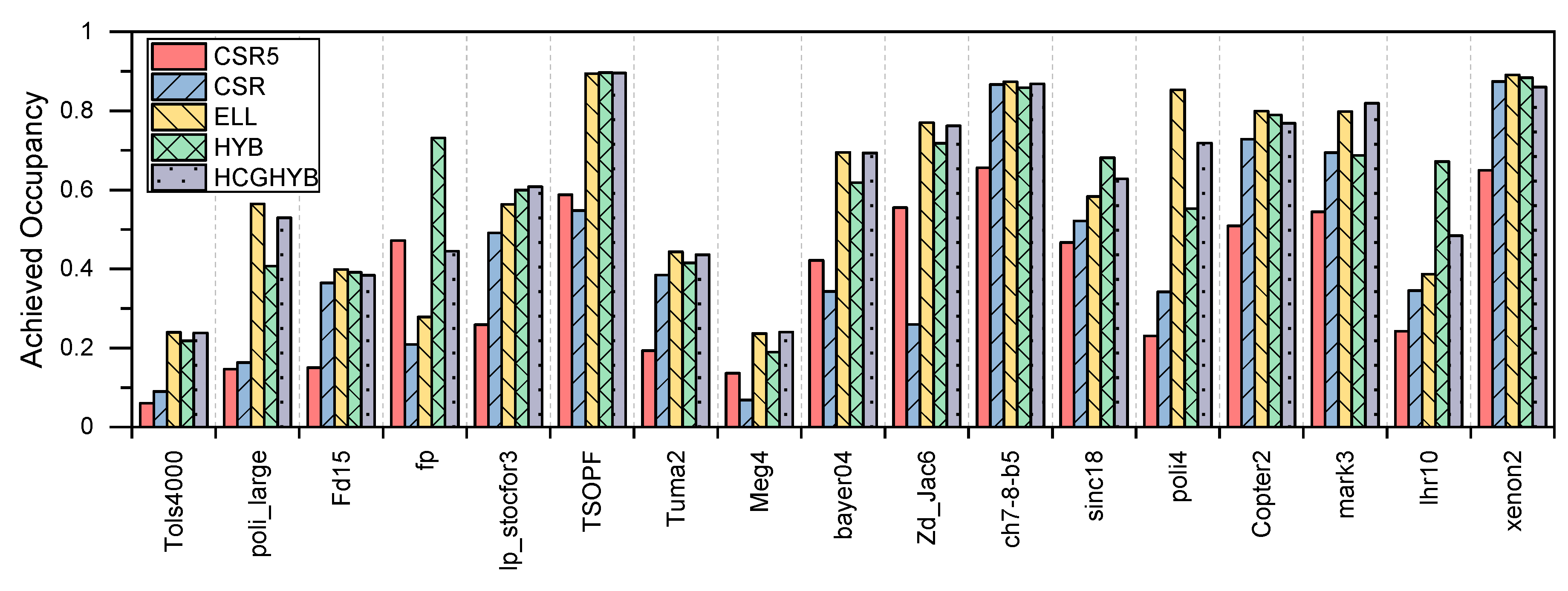
8.2.3. GPU Utilization
9. Conclusions and Future Work
Author Contributions
Funding
Acknowledgments
Conflicts of Interest
References
- Asanovic, K.; Bodik, R.; Catanzaro, B.C.; Gebis, J.J.; Husbands, P.; Keutzer, K.; Patterson, D.A.; Plishker, W.L.; Shalf, J.; Williams, S.W.; et al. The Landscape of Parallel Computing Research: A View from Berkeley; Technical Report UCB/EECS-2006-183; EECS Department, University of California: Berkeley, CA, USA, 2006. [Google Scholar]
- Davis, T.A.; Hu, Y. The University of Florida Sparse Matrix Collection. ACM Trans. Math. Softw. 2011, 38, 1:1–1:25. [Google Scholar] [CrossRef]
- Yang, W.; Li, K.; Li, K. A hybrid computing method of SpMV on CPU–GPU heterogeneous computing systems. J. Parallel Distrib. Comput. 2017, 104, 49–60. [Google Scholar] [CrossRef]
- Huan, G.; Qian, Z. A new method of Sparse Matrix-Vector Multiplication on GPU. In Proceedings of the 2012 2nd International Conference on Computer Science and Network Technology, Changchun, China, 29–31 December 2012. [Google Scholar] [CrossRef]
- Hassani, R.; Fazely, A.; Choudhury, R.U.A.; Luksch, P. Analysis of Sparse Matrix-Vector Multiplication Using Iterative Method in CUDA. In Proceedings of the 2013 IEEE Eighth International Conference on Networking, Architecture and Storage, Xi’an, China, 17–19 July 2013. [Google Scholar] [CrossRef]
- Guo, P.; Wang, L. Auto-Tuning CUDA Parameters for Sparse Matrix-Vector Multiplication on GPUs. In Proceedings of the 2010 International Conference on Computational and Information Sciences, Chengdu, China, 17–19 December 2010. [Google Scholar] [CrossRef]
- Merrill, D.; Garland, M. Merge-Based Parallel Sparse Matrix-Vector Multiplication. In Proceedings of the SC16: International Conference for High Performance Computing, Networking, Storage and Analysis, Salt Lake City, UT, USA, 13–18 November 2016. [Google Scholar] [CrossRef]
- Ahamed, A.K.C.; Magoulès, F. Efficient implementation of Jacobi iterative method for large sparse linear systems on graphic processing units. J. Supercomput. 2016, 73, 3411–3432. [Google Scholar] [CrossRef]
- Hou, K.; Feng, W.-C.; Che, S. Auto-Tuning Strategies for Parallelizing Sparse Matrix-Vector (SpMV) Multiplication on Multi- and Many-Core Processors. In Proceedings of the 2017 IEEE International Parallel and Distributed Processing Symposium Workshops (IPDPSW), Lake Buena Vista, FL, USA, 29 May–2 June 2017. [Google Scholar] [CrossRef]
- Langville, A.N.; Meyer, C.D. A survey of eigenvector methods for web information retrieval. SIAM Rev. 2005, 47, 135–161. [Google Scholar] [CrossRef]
- Kamvar, S.D.; Haveliwala, T.H.; Manning, C.D.; Golub, G.H. Extrapolation methods for accelerating PageRank computations. In Proceedings of the 12th International Conference on World Wide Web; ACM: New York, NY, USA, 2003; pp. 261–270. [Google Scholar]
- Heffes, H.; Lucantoni, D. A Markov Modulated Characterization of Packetized Voice and Data Traffic and Related Statistical Multiplexer Performance. IEEE J. Sel. Areas Commun. 1986, 4, 856–868. [Google Scholar] [CrossRef]
- Bylina, J.; Bylina, B.; Karwacki, M. An efficient representation on GPU for transition rate matrices for Markov chains. In Parallel Processing and Applied Mathematics; Springer: Berlin, Germany, 2013. [Google Scholar]
- Bylina, J.; Bylina, B.; Karwacki, M. A Markovian Model of a Network of Two Wireless Devices. Comput. Netw. 2012. [Google Scholar] [CrossRef]
- Ahamed, A.K.C.; Magoules, F. Fast sparse matrix-vector multiplication on graphics processing unit for finite element analysis. In Proceedings of the 2012 IEEE 14th International Conference on High Performance Computing and Communication & 2012 IEEE 9th International Conference on Embedded Software and Systems, Liverpool, UK, 25–27 June 2012. [Google Scholar] [CrossRef]
- Yu, J.; Lukefahr, A.; Palframan, D.; Dasika, G.; Das, R.; Mahlke, S. Scalpel: Customizing DNN Pruning to the Underlying Hardware Parallelism. In Proceedings of the 44th Annual International Symposium on Computer Architecture; Association for Computing Machinery: New York, NY, USA, 2017; pp. 548–560. [Google Scholar] [CrossRef]
- Mohammed, T.; Joe-Wong, C.; Babbar, R.; Francesco, M.D. Distributed Inference Acceleration with Adaptive DNN Partitioning and Offloading. In Proceedings of the IEEE INFOCOM 2020—IEEE Conference on Computer Communications, Toronto, ON, Canada, 6–9 July 2020; pp. 854–863. [Google Scholar] [CrossRef]
- Benatia, A.; Ji, W.; Wang, Y.; Shi, F. BestSF: A Sparse Meta-Format for Optimizing SpMV on GPU. ACM Trans. Archit. Code Optim. 2018, 15. [Google Scholar] [CrossRef]
- Abdali, S.K.; Wise, D.S. Experiments with quadtree representation of matrices. In Proceedings of the Symbolic and Algebraic Computation International Symposium ISSAC ’88, Rome, Italy, 4–8 July 1988; Springer: Berlin/Heidelberg, Germany, 1989; pp. 96–108. [Google Scholar] [CrossRef]
- Langr, D.; Simecek, I.; Tvrdik, P. Storing sparse matrices to files in the adaptive-blocking hierarchical storage format. In Proceedings of the 2013 Federated Conference on Computer Science and Information Systems (FedCSIS), Krakow, Poland, 8–11 September 2013; pp. 479–486. [Google Scholar]
- Simecek, I.; Langr, D.; Tvrdík, P. Space efficient formats for structure of sparse matrices based on tree structures. In Proceedings of the 2013 15th International Symposium on Symbolic and Numeric Algorithms for Scientific Computing (SYNASC), Timisoara, Romania, 23–26 September 2013; pp. 344–351. [Google Scholar]
- Simecek, I.; Langr, D. Tree-based space efficient formats for storing the structure of sparse matrices. Scalable Comput. Pract. Exp. 2014, 15, 1–20. [Google Scholar]
- Zhang, J.; Wan, J.; Li, F.; Mao, J.; Zhuang, L.; Yuan, J.; Liu, E.; Yu, Z. Efficient sparse matrix–vector multiplication using cache oblivious extension quadtree storage format. Future Gener. Comput. Syst. 2016, 54, 490–500. [Google Scholar]
- Meyer, J.C.; Natvig, L.; Karakasis, V.; Siakavaras, D.; Nikas, K. Energy-efficient Sparse Matrix Auto-tuning with CSX. In Proceedings of the 27th IEEE International Parallel & Distributed Processing Symposium Workshops & PhD Forum (IPDPSW), Cambridge, MA, USA, 20–24 May 2013. [Google Scholar]
- Elafrou, A.; Goumas, G.I.; Koziris, N. A lightweight optimization selection method for Sparse Matrix-Vector Multiplication. CoRR 2015, arXiv:1511.02494. [Google Scholar]
- Shaikh, M.A.H.; Hasan, K.M.A. Efficient storage scheme for n-dimensional sparse array: GCRS/GCCS. In Proceedings of the 2015 International Conference on High Performance Computing Simulation (HPCS), Amsterdam, The Netherlands, 20–24 July 2015; pp. 137–142. [Google Scholar] [CrossRef]
- Martone, M.; Filippone, S.; Tucci, S.; Paprzycki, M.; Ganzha, M. Utilizing Recursive Storage in Sparse Matrix-Vector Multiplication-Preliminary Considerations. In CATA; ISCA: Honolulu, HI, USA, 2010; pp. 300–305. [Google Scholar]
- Martone, M. Efficient multithreaded untransposed, transposed or symmetric sparse matrix–vector multiplication with the recursive sparse blocks format. Parallel Comput. 2014, 40, 251–270. [Google Scholar] [CrossRef][Green Version]
- Guo, D.; Gropp, W. Applications of the streamed storage format for sparse matrix operations. Int. J. High Perform. Comput. Appl. 2014, 28, 3–12. [Google Scholar] [CrossRef]
- Bakos, J.D.; Nagar, K.K. Exploiting Matrix Symmetry to Improve FPGA-Accelerated Conjugate Gradient. In Proceedings of the 2009 17th IEEE Symposium on Field Programmable Custom Computing Machines; IEEE Computer Society: Washington, DC, USA, 2009; pp. 223–226. [Google Scholar] [CrossRef]
- Grigoras, P.; Burovskiy, P.; Hung, E.; Luk, W. Accelerating SpMV on FPGAs by Compressing Nonzero Values. In Proceedings of the 2015 IEEE 23rd Annual International Symposium on Field-Programmable Custom Computing Machines; IEEE Computer Society: Washington, DC, USA, 2015; pp. 64–67. [Google Scholar] [CrossRef]
- Boland, D.; Constantinides, G.A. Optimizing Memory Bandwidth Use and Performance for Matrix-vector Multiplication in Iterative Methods. ACM Trans. Reconfigurable Technol. Syst. 2011, 4, 22:1–22:14. [Google Scholar] [CrossRef]
- Kestur, S.; Davis, J.D.; Chung, E.S. Towards a Universal FPGA Matrix-Vector Multiplication Architecture. In Proceedings of the 2012 IEEE 20th International Symposium on Field-Programmable Custom Computing Machines; IEEE Computer Society: Washington, DC, USA, 2012; pp. 9–16. [Google Scholar] [CrossRef]
- DeLorimier, M.; DeHon, A. Floating-point Sparse Matrix-vector Multiply for FPGAs. In Proceedings of the 2005 ACM/SIGDA 13th International Symposium on Field-Programmable Gate Arrays; ACM: New York, NY, USA, 2005; pp. 75–85. [Google Scholar] [CrossRef]
- Dorrance, R.; Ren, F.; Marković, D. A Scalable Sparse Matrix-vector Multiplication Kernel for Energy-efficient Sparse-blas on FPGAs. In Proceedings of the 2014 ACM/SIGDA International Symposium on Field-programmable Gate Arrays; ACM: New York, NY, USA, 2014; pp. 161–170. [Google Scholar] [CrossRef]
- Grigoraş, P.; Burovskiy, P.; Luk, W.; Sherwin, S. Optimising Sparse Matrix Vector multiplication for large scale FEM problems on FPGA. In Proceedings of the 2016 26th International Conference on Field Programmable Logic and Applications (FPL), Lausanne, Switzerland, 29 August–2 September 2016; pp. 1–9. [Google Scholar] [CrossRef]
- Kuzmanov, G.; Taouil, M. Reconfigurable sparse/dense matrix-vector multiplier. In Proceedings of the 2009 International Conference on Field-Programmable Technology, Sydney, Australia, 9–11 December 2009; pp. 483–488. [Google Scholar] [CrossRef]
- Yan, S.; Li, C.; Zhang, Y.; Zhou, H. yaSpMV: Yet Another SpMV Framework on GPUs; ACM SIGPLAN Notices; ACM: New York, NY, USA, 2014; Volume 49, pp. 107–118. [Google Scholar]
- Liu, W.; Vinter, B. CSR5: An Efficient Storage Format for Cross-Platform Sparse Matrix-Vector Multiplication. In Proceedings of the 29th ACM on International Conference on Supercomputing; ACM: New York, NY, USA, 2015; pp. 339–350. [Google Scholar] [CrossRef]
- Liu, X.; Smelyanskiy, M.; Chow, E.; Dubey, P. Efficient sparse matrix-vector multiplication on x86-based many-core processors. In Proceedings of the 27th International ACM Conference on International Conference on Supercomputing; ACM: New York, NY, USA, 2013; pp. 273–282. [Google Scholar]
- Saule, E.; Kaya, K.; Çatalyürek, Ü.V. Performance Evaluation of Sparse Matrix Multiplication Kernels on Intel Xeon Phi. In Parallel Processing and Applied Mathematics, Proceedings of the 10th International Conference, PPAM 2013, Warsaw, Poland, 8–11 September 2013; Wyrzykowski, R., Dongarra, J., Karczewski, K., Waśniewski, J., Eds.; Revised Selected Papers, Part I; Springer: Berlin/Heidelberg, Germany, 2014; pp. 559–570. [Google Scholar] [CrossRef]
- Kreutzer, M.; Hager, G.; Wellein, G.; Fehske, H.; Bishop, A.R. A unified sparse matrix data format for efficient general sparse matrix-vector multiplication on modern processors with wide SIMD units. SIAM J. Sci. Comput. 2014, 36, C401–C423. [Google Scholar] [CrossRef]
- Yzelman, A.N. Generalised Vectorisation for Sparse Matrix: Vector Multiplication. In Proceedings of the 5th Workshop on Irregular Applications: Architectures and Algorithms; ACM: New York, NY, USA, 2015; pp. 6:1–6:8. [Google Scholar] [CrossRef]
- Tang, W.T.; Zhao, R.; Lu, M.; Liang, Y.; Huynh, H.P.; Li, X.; Goh, R.S.M. Optimizing and Auto-tuning Scale-free Sparse Matrix-vector Multiplication on Intel Xeon Phi. In Proceedings of the 13th Annual IEEE/ACM International Symposium on Code Generation and Optimization; IEEE Computer Society: Washington, DC, USA, 2015; pp. 136–145. [Google Scholar]
- Cheng, J.R.; Gen, M. Accelerating genetic algorithms with GPU computing: A selective overview. Comput. Ind. Eng. 2019, 128, 514–525. [Google Scholar] [CrossRef]
- Jeon, M.; Venkataraman, S.; Phanishayee, A.; Qian, J.; Xiao, W.; Yang, F. Analysis of large-scale multi-tenant {GPU} clusters for {DNN} training workloads. In Proceedings of the 2019 {USENIX} Annual Technical Conference ({USENIX}{ATC} 19), Renton, WA, USA, 10 July 2019; pp. 947–960. [Google Scholar]
- Aqib, M.; Mehmood, R.; Alzahrani, A.; Katib, I.; Albeshri, A.; Altowaijri, S.M. Smarter Traffic Prediction Using Big Data, In-Memory Computing, Deep Learning and GPUs. Sensors 2019, 19, 2206. [Google Scholar] [CrossRef]
- Aqib, M.; Mehmood, R.; Alzahrani, A.; Katib, I.; Albeshri, A.; Altowaijri, S.M. Rapid Transit Systems: Smarter Urban Planning Using Big Data, In-Memory Computing, Deep Learning, and GPUs. Sustainability 2019, 11, 2736. [Google Scholar] [CrossRef]
- Magoulès, F.; Ahamed, A.K.C. Alinea: An Advanced Linear Algebra Library for Massively Parallel Computations on Graphics Processing Units. Int. J. High Perform. Comput. Appl. 2015, 29, 284–310. [Google Scholar] [CrossRef]
- Muhammed, T.; Mehmood, R.; Albeshri, A.; Katib, I. UbeHealth: A Personalized Ubiquitous Cloud and Edge-Enabled Networked Healthcare System for Smart Cities. IEEE Access 2018, 6, 32258–32285. [Google Scholar] [CrossRef]
- Kirk, D.B.; Hwu, W.M.W. Programming Massively Parallel Processors: A Hands-on Approach, 1st ed.; Morgan Kaufmann Publishers Inc.: San Francisco, CA, USA, 2010. [Google Scholar]
- Owens, J.; Houston, M.; Luebke, D.; Green, S.; Stone, J.; Phillips, J. GPU Computing. Proc. IEEE 2008, 96, 879–899. [Google Scholar] [CrossRef]
- Fevgas, A.; Daloukas, K.; Tsompanopoulou, P.; Bozanis, P. Efficient solution of large sparse linear systems in modern hardware. In Proceedings of the 2015 6th International Conference on Information, Intelligence, Systems and Applications (IISA), Corfu, Greece, 6–8 July 2015. [Google Scholar] [CrossRef]
- Nisa, I.; Siegel, C.; Rajam, A.S.; Vishnu, A.; Sadayappan, P. Effective Machine Learning Based Format Selection and Performance Modeling for SpMV on GPUs. In Proceedings of the 2018 IEEE International Parallel and Distributed Processing Symposium Workshops (IPDPSW), Vancouver, BC, Canada, 21–25 May 2018; pp. 1056–1065. [Google Scholar] [CrossRef]
- Filippone, S.; Cardellini, V.; Barbieri, D.; Fanfarillo, A. Sparse Matrix-Vector Multiplication on GPGPUs. ACM Trans. Math. Softw. 2017, 43, 1–49. [Google Scholar] [CrossRef]
- Bell, N.; Garland, M. Efficient Sparse Matrix-Vector Multiplication on CUDA; Techreport NVR-2008-004; Nvidia Corporation: Santa Clara, CA, USA, 2008. [Google Scholar]
- Choi, J.W.; Singh, A.; Vuduc, R.W. Model-driven Autotuning of Sparse Matrix-vector Multiply on GPUs. SIGPLAN Not. 2010, 45, 115–126. [Google Scholar] [CrossRef]
- Flegar, G.; Anzt, H. Overcoming Load Imbalance for Irregular Sparse Matrices. In Proceedings of the Seventh Workshop on Irregular Applications: Architectures and Algorithms; ACM: New York, NY, USA, 2017; pp. 2:1–2:8. [Google Scholar] [CrossRef]
- Ashari, A.; Sedaghati, N.; Eisenlohr, J.; Parthasarathy, S.; Sadayappan, P. Fast Sparse Matrix-vector Multiplication on GPUs for Graph Applications. In Proceedings of the International Conference for High Performance Computing, Networking, Storage and Analysis; IEEE Press: Piscataway, NJ, USA, 2014; pp. 781–792. [Google Scholar] [CrossRef]
- Su, B.Y.; Keutzer, K. clSpMV: A Cross-Platform OpenCL SpMV Framework on GPUs. In Proceedings of the 26th ACM International Conference on Supercomputing; ACM: New York, NY, USA, 2012; pp. 353–364. [Google Scholar] [CrossRef]
- Guo, P.; Wang, L.; Chen, P. A Performance Modeling and Optimization Analysis Tool for Sparse Matrix-Vector Multiplication on GPUs. IEEE Trans. Parallel Distrib. Syst. 2014, 25, 1112–1123. [Google Scholar] [CrossRef]
- Li, J.; Tan, G.; Chen, M.; Sun, N. SMAT: An Input Adaptive Auto-tuner for Sparse Matrix-vector Multiplication. SIGPLAN Not. 2013, 48, 117–126. [Google Scholar] [CrossRef]
- Sedaghati, N.; Mu, T.; Pouchet, L.N.; Parthasarathy, S.; Sadayappan, P. Automatic Selection of Sparse Matrix Representation on GPUs. In Proceedings of the 29th ACM on International Conference on Supercomputing; ACM: New York, NY, USA, 2015; pp. 99–108. [Google Scholar] [CrossRef]
- Benatia, A.; Ji, W.; Wang, Y.; Shi, F. Sparse Matrix Format Selection with Multiclass SVM for SpMV on GPU. In Proceedings of the 2016 45th International Conference on Parallel Processing (ICPP), Philadelphia, PA, USA, 16–19 August 2016; pp. 496–505. [Google Scholar] [CrossRef]
- Li, K.; Yang, W.; Li, K. Performance Analysis and Optimization for SpMV on GPU Using Probabilistic Modeling. IEEE Trans. Parallel Distrib. Syst. 2015, 26, 196–205. [Google Scholar] [CrossRef]
- Kwiatkowska, M.; Parker, D.; Zhang, Y.; Mehmood, R. Dual-Processor Parallelisation of Symbolic Probabilistic Model Checking. In Proceedings of the IEEE Computer Society’s 12th Annual International Symposium on Modeling, Analysis, and Simulation of Computer and Telecommunications Systems; IEEE Computer Society: Washington, DC, USA, 2004; pp. 123–130. [Google Scholar]
- Mehmood, R.; Parker, D.; Kwiatkowska, M. An Efficient BDD-Based Implementation of Gauss-Seidel for CTMC Analysis; Technical Report CSR-03-13; School of Computer Science, University of Birmingham: Birmingham, UK, 2003. [Google Scholar]
- Mehmood, R.; Crowcroft, J. Parallel Iterative Solution Method for Large Sparse Linear Equation Systems; Technical Report UCAM-CL-TR-650; University of Cambridge, Computer Laboratory: Cambridge, UK, 2005. [Google Scholar]
- Mehmood, R.; Crowcroft, J.; Elmirghani, J.M.H. A Parallel Implicit Method for the Steady-State Solution of CTMCs. In Proceedings of the 14th IEEE International Symposium on Modeling, Analysis, and Simulation, Monterey, CA, USA, 11–14 September 2006; pp. 293–302. [Google Scholar]
- Mehmood, R.; Lu, J.A. Computational Markovian Analysis of Large Systems. J. Manuf. Technol. Manag. 2011, 22, 804–817. [Google Scholar] [CrossRef]
- Usman, S.; Mehmood, R.; Katib, I.; Albeshri, A.; Altowaijri, S. ZAKI: A Smart Method and Tool for Automatic Performance Optimization of Parallel SpMV Computations on Distributed Memory Machines. Mob. Networks Appl. 2019. [Google Scholar] [CrossRef]
- Usman, S.; Mehmood, R.; Katib, I.; Albeshri, A. ZAKI+: A Machine Learning Based Process Mapping Tool for SpMV Computations on Distributed Memory Architectures. IEEE Access 2019, 7, 81279–81296. [Google Scholar] [CrossRef]
- Alyahya, H.; Mehmood, R.; Katib, I. Parallel Sparse Matrix Vector Multiplication on Intel MIC: Performance Analysis. In Smart Societies, Infrastructure, Technologies and Applications; Mehmood, R., Bhaduri, B., Katib, I., Chlamtac, I., Eds.; Springer International Publishing: Cham, Switzerland, 2018; pp. 306–322. [Google Scholar]
- Alyahya, H.; Mehmood, R.; Katib, I. Parallel Iterative Solution of Large Sparse Linear Equation Systems on the Intel MIC Architecture. In Smart Infrastructure and Applications: Foundations for Smarter Cities and Societies; Mehmood, R., See, S., Katib, I., Chlamtac, I., Eds.; Springer International Publishing: Cham, Switzerland, 2020; pp. 377–407. [Google Scholar] [CrossRef]
- Alzahrani, S.; Ikbal, M.R.; Mehmood, R.; Fayez, M.; Katib, I. Performance Evaluation of Jacobi Iterative Solution for Sparse Linear Equation System on Multicore and Manycore Architectures. In Smart Societies, Infrastructure, Technologies and Applications; Mehmood, R., Bhaduri, B., Katib, I., Chlamtac, I., Eds.; Springer International Publishing: Cham, Switzerland, 2018; pp. 296–305. [Google Scholar]
- AlAhmadi, S.; Muhammed, T.; Mehmood, R.; Albeshri, A. Performance Characteristics for Sparse Matrix-Vector Multiplication on GPUs. In Smart Infrastructure and Applications: Foundations for Smarter Cities and Societies; Mehmood, R., See, S., Katib, I., Chlamtac, I., Eds.; Springer International Publishing: Cham, Switzerland, 2020; pp. 409–426. [Google Scholar] [CrossRef]
- Muhammed, T.; Mehmood, R.; Albeshri, A.; Katib, I. SURAA: A Novel Method and Tool for Loadbalanced and Coalesced SpMV Computations on GPUs. Appl. Sci. 2019, 9, 947. [Google Scholar] [CrossRef]
- El-Gorashi, T.; Pranggono, B.; Mehmood, R.; Elmirghani, J. A Mirroring Strategy for SANs in a Metro WDM Sectioned Ring Architecture under Different Traffic Scenarios. J. Opt. Commun. 2008, 29, 89–97. [Google Scholar] [CrossRef]
- Mehmood, R.; Alturki, R.; Zeadally, S. Multimedia applications over metropolitan area networks (MANs). J. Netw. Comput. Appl. 2011, 34, 1518–1529. [Google Scholar] [CrossRef]
- Mehmood, R.; Graham, G. Big Data Logistics: A health-care Transport Capacity Sharing Model. Procedia Comput. Sci. 2015, 64, 1107–1114. [Google Scholar] [CrossRef]
- Mehmood, R.; Meriton, R.; Graham, G.; Hennelly, P.; Kumar, M. Exploring the Influence of Big Data on City Transport Operations: A Markovian Approach. Int. J. Oper. Prod. Manag. 2017, 37, 75–104. [Google Scholar] [CrossRef]
- El-Gorashi, T.E.H.; Pranggono, B.; Mehmood, R.; Elmirghani, J.M.H. A data Mirroring technique for SANs in a Metro WDM sectioned ring. In Proceedings of the 2008 International Conference on Optical Network Design and Modeling, Vilanova i la Geltru, Spain, 12–14 March 2008; pp. 1–6. [Google Scholar] [CrossRef]
- Pranggono, B.; Mehmood, R.; Elmirghani, J.M.H. Performance Evaluation of a Metro WDM Multi-channel Ring Network with Variable-length Packets. In Proceedings of the 2007 IEEE International Conference on Communications, Glasgow, UK, 24–28 June 2007; pp. 2394–2399. [Google Scholar] [CrossRef]
- Altowaijri, S.; Mehmood, R.; Williams, J. A Quantitative Model of Grid Systems Performance in Healthcare Organisations. In Proceedings of the 2010 International Conference on Intelligent Systems, Modelling and Simulation, Liverpool, UK, 27–29 January 2010; pp. 431–436. [Google Scholar]
- Kwiatkowska, M.; Mehmood, R.; Norman, G.; Parker, D. A Symbolic Out-of-Core Solution Method for Markov Models. Electron. Notes Theor. Comput. Sci. 2002, 68, 589–604. [Google Scholar] [CrossRef]
- Langr, D.; Tvrdik, P. Evaluation Criteria for Sparse Matrix Storage Formats. IEEE Trans. Parallel Distrib. Syst. 2016, 27, 428–440. [Google Scholar] [CrossRef]
- Abu-Sufah, W.; Karim, A.A. An Effective Approach for Implementing Sparse Matrix-Vector Multiplication on Graphics Processing Units. In Proceedings of the 2012 IEEE 14th International Conference on High Performance Computing and Communication & 2012 IEEE 9th International Conference on Embedded Software and Systems; IEEE Computer Society: Washington, DC, USA, 2012; pp. 453–460. [Google Scholar] [CrossRef]
- Professional CUDA C Programming, 1st ed.; Wrox Press Ltd.: Birmingham, UK, 2014.
- Profiler User’s Guide. Available online: https://docs.nvidia.com/cuda/profiler-users-guide/index.html (accessed on 12 October 2020).
- Saad, Y. SPARSKIT: A Basic Tool Kit for Sparse Matrix Computations—Version 2. 1994. Available online: https://www-users.cs.umn.edu/~saad/software/SPARSKIT/ (accessed on 12 October 2020).
- Grimes, R.G.; Kincaid, D.R.; Young, D.M. ITPACK 2.0 User’S Guide; Center for Numerical Analysis, The University of Texas at Austin: Austin, TX, USA, 1979. [Google Scholar]
- Mittal, S.; Vetter, J.S. A Survey of CPU-GPU Heterogeneous Computing Techniques. ACM Comput. Surv. 2015, 47. [Google Scholar] [CrossRef]
- Benatia, A.; Ji, W.; Wang, Y.; Shi, F. Sparse matrix partitioning for optimizing SpMV on CPU-GPU heterogeneous platforms. Int. J. High Perform. Comput. Appl. 2020, 34, 66–80. [Google Scholar] [CrossRef]


| Structure | Matrix Name | Rows | Columns | Application Domain | |||||
|---|---|---|---|---|---|---|---|---|---|
 | bayer04 | 20,545 | 20,545 | 159,082 | 8.2 | 7 | 34 | 4115.99 | Chemical Simulation |
 | ch7-8-b5 | 141,120 | 141,120 | 846,720 | 0 | 6 | 6 | 40,549.39 | Combinatorics |
 | copter2 | 55,476 | 55,476 | 407,714 | 3.55 | 7 | 20 | 28,217.87 | Computational Fluid Dynamics |
 | fd15 | 11,532 | 11,532 | 44,206 | 1.65 | 3 | 6 | 2690.89 | Materials |
 | Fp | 7548 | 7548 | 848,553 | 207.83 | 112 | 957 | 6388.57 | Electromagnetics |
 | lhr10 | 10,672 | 10,672 | 232,633 | 26.37 | 21 | 63 | 3380.56 | Chemical Simulation |
 | lp_stocfor3 | 16,675 | 23,541 | 76,473 | 3.34 | 4 | 15 | 3123.99 | Linear Programming |
 | mark3jac120 | 54,929 | 54,929 | 342,475 | 4.36 | 6 | 44 | 1960.54 | Economics |
 | Meg4 | 5860 | 5860 | 26,324 | 16.66 | 4 | 1193 | 1758.92 | Circuit Simulation |
 | poli4 | 15,575 | 15,575 | 33,074 | 8.93 | 2 | 491 | 261.04 | Economics |
 | poli_large | 33,833 | 33,833 | 73,249 | 7.57 | 2 | 304 | 248.12 | Economics |
 | sinc18 | 16,428 | 16,428 | 973,826 | 34.32 | 59 | 111 | 4369.81 | Materials |
 | Tols4000 | 4000 | 4000 | 8784 | 5.92 | 2 | 90 | 1130.87 | Computational Fluid Dynamics |
 | TSOPF_RS_b300_c2 | 28,338 | 28,338 | 2943,887 | 102.4 | 103 | 209 | 25,564.97 | Power Network |
 | Tuma2 | 12,992 | 12,992 | 28,440 | 1.2 | 2 | 5 | 4226.74 | 2D/3D |
 | xenon2 | 157,464 | 157,464 | 3866,688 | 4.11 | 24 | 27 | 4934.59 | Materials |
 | Zd_Jac6 | 22,835 | 22,835 | 1711,983 | 175.49 | 74 | 1050 | 3436.54 | Chemical Simulation |
| nnz | npr variance | distavg | anpr | maxnpr | |
|---|---|---|---|---|---|
| CSR | medium | high | medium | medium | high |
| ELL | medium | high | low | medium | high |
| HYB | medium | medium | low | medium | medium |
| CSR5 | medium | low | low | medium | low |
© 2020 by the authors. Licensee MDPI, Basel, Switzerland. This article is an open access article distributed under the terms and conditions of the Creative Commons Attribution (CC BY) license (http://creativecommons.org/licenses/by/4.0/).
Share and Cite
AlAhmadi, S.; Mohammed, T.; Albeshri, A.; Katib, I.; Mehmood, R. Performance Analysis of Sparse Matrix-Vector Multiplication (SpMV) on Graphics Processing Units (GPUs). Electronics 2020, 9, 1675. https://doi.org/10.3390/electronics9101675
AlAhmadi S, Mohammed T, Albeshri A, Katib I, Mehmood R. Performance Analysis of Sparse Matrix-Vector Multiplication (SpMV) on Graphics Processing Units (GPUs). Electronics. 2020; 9(10):1675. https://doi.org/10.3390/electronics9101675
Chicago/Turabian StyleAlAhmadi, Sarah, Thaha Mohammed, Aiiad Albeshri, Iyad Katib, and Rashid Mehmood. 2020. "Performance Analysis of Sparse Matrix-Vector Multiplication (SpMV) on Graphics Processing Units (GPUs)" Electronics 9, no. 10: 1675. https://doi.org/10.3390/electronics9101675
APA StyleAlAhmadi, S., Mohammed, T., Albeshri, A., Katib, I., & Mehmood, R. (2020). Performance Analysis of Sparse Matrix-Vector Multiplication (SpMV) on Graphics Processing Units (GPUs). Electronics, 9(10), 1675. https://doi.org/10.3390/electronics9101675