Radio–Image Transformer: Bridging Radio Modulation Classification and ImageNet Classification

Abstract

Radio modulation classification is widely used in the field of wireless communication. In this paper, in order to realize radio modulation classification with the help of the existing ImageNet classification models, we propose a radio–image transformer which extracts the instantaneous amplitude, instantaneous phase and instantaneous frequency from the received radio complex baseband signals, then converts the signals into images by the proposed signal rearrangement method or convolution mapping method. We finally use the existing ImageNet classification network models to classify the modulation type of the signal. The experimental results show that the proposed signal rearrangement method and convolution mapping method are superior to the methods using constellation diagrams and time–frequency images, which shows their performance advantages. In addition, by comparing the results of the seven ImageNet classification network models, it can be seen that, except for the relatively poor performance of the architecture MNASNet1_0, the modulation classification performance obtained by the other six network architectures is similar, indicating that the proposed methods do not have high requirements for the architecture of the selected ImageNet classification network models. Moreover, the experimental results show that our method has good classification performance for signal datasets with different sampling rates, Orthogonal Frequency Division Multiplexing (OFDM) signals and real measured signals.

1. Introduction

Radio signal classification is widely used in the field of communication. For example, in cognitive radio [1], the secondary user needs to monitor the primary user’s signal to avoid harmful interference to the primary user. Therefore, the secondary user needs to classify the primary user’s signal to accurately know the type of primary user currently using the spectrum, so as to access the spectrum in a more efficient manner [2]. In electromagnetic spectrum management [3,4], some malicious users may transmit specific signals to disturb the spectrum use. In these circumstances with the overlapping and coexistence of various radio signals, if each radio signal can be identified, it will help to determine the existence of malicious users, and then take effective measures to deal with the situation. In adaptive modulation and coding communication [5,6,7], if the receiver is able to recognize the modulation and coding scheme adopted by the transmitter, it can choose the corresponding demodulation and decoding algorithm for information recovery, so as to save signaling overhead for informing the receiver of the adopted modulation and coding scheme. Modulation type is a basic attribute of radio communication signal, and in this paper, we mainly focus on radio modulation classification.

The purpose of the radio modulation classification problem is to identify the type of modulation to which the signal belongs. This is actually a multi-category classification problem, and the number of categories is the number of modulation types in the signal dataset.

In this paper, we treat the problem of radio modulation classification by making full use of the existing mature ImageNet classification network structure. Since the raw radio signals are represented in IQ form, which is different from the image, we propose a radio–image transformer (RIT) to convert the radio signal into the image format. To be specific, we firstly extract the instantaneous amplitude, instantaneous phase and instantaneous frequency of the radio IQ signals, and then convert the signals into images by the proposed signal rearrangement method (SRM) or convolution mapping method (CMM). We finally complete the task of signal modulation classification by using the existing ImageNet classification network models. We verify the effectiveness of the proposed methods through simulations.

The main contribution of this paper is that the RIT proposed can transform the signal classification problem into the image classification problem by mapping signals to images, and thus complete the radio signal modulation recognition using sophisticated classification techniques in the image field. We will show by extensive experiments that our method achieves better classification accuracy than some existing signal-to-image classification methods.

The rest of the paper is organized as follows. Section 2 gives the related work and literature review. Section 3 presents the definition of radio modulation classification problem. Section 4 introduces the proposed radio modulation classification methods. Section 5 introduces the experiments and performance evaluation. Section 6 summarizes the paper.

2. Related Work and Literature Review

In this section, we mainly introduce some related work of radio modulation classification. The traditional modulation classification methods are mainly based on feature design [8,9,10,11,12,13]. The quality of the designed features directly determines the quality of recognition performance. However, these designed features are often associated with a specific modulation, and it is difficult to find features that are widely applicable to a variety of modulations. As an end-to-end learning method, deep learning [14] unifies feature extraction and recognition tasks, avoids the process of manual feature design, and hence greatly enhances its universal applicability. For instance, in the field of image recognition, a lot of convolutional neural network (CNN) structures have been designed for the ImageNet dataset [15] and these CNNs achieved pretty good classification performance. In view of the great success of deep learning in image classification and other fields, more and more work has introduced deep learning into radio modulation recognition. These methods can be divided into two categories. The first is to design a special CNN or long short term memory (LSTM) network for modulation classification according to the raw radio signals’ input form (the in-phase and quadrature (IQ) form) [16,17,18,19]. The second is to convert the radio signals into images, and then classify the images by referring to the network structure used for image classification, so as to realize the classification of radio signals. At present, there are two main ways to transform IQ signals into images, namely, constellation diagrams [20] and time–frequency images [21,22,23], but they may affect the modulation classification performance due to the loss of the temporal correlation information between signal sampling points.

The classification methods proposed in this paper make full use of the technology in the field of image classification, especially the content related to ImageNet. ImageNet is an image dataset widely used by computer vision researchers and plays an important role in object detection and recognition and other fields. The image dataset was created by Professor Li’s team. At that time, the academic scholars mostly focused on designing better algorithms. Prof. Li, however, believed that a good dataset is beneficial to the training of models and then began to collect images with annotated information on a large scale and finally officially launched the ImageNet dataset in 2009. This dataset contains about 15 million annotated images, which can be divided into about 22,000 categories [15]. The dataset can be used to train the models to improve their performance, which makes a great contribution to the academic research in this area.

In 2010, the ImageNet Large Scale Visual Recognition Challenge (ILSVRC), based on the ImageNet dataset, was launched globally. The competition includes image classification, target detection, target positioning, scene classification and video target detection, and so on. A subset of the ImageNet dataset is used in this competition, which contains 1000 categories, and each category contains about 1000 images. Various classic CNN models, such as AlexNet [24], ZFNet [25], VGG [26], GoogleNet [27] and ResNet [28], emerged in the ILSVRC competitions held for 7 years. In particular, ResNet learns the residual representation between inputs and outputs by using multiple layers that contain parameters and can be learned, thus avoiding the problem of gradient disappearance and making the model easier to optimize. In the field of image classification, the CNN models trained with a large amount of high-quality images can be transferred to other image datasets for classification and recognition, and they can also be fine-tuned and trained on this basis. The advantage of this is that it is unnecessary to train the neural network from scratch, which can save time and computing resources. Most of the classic CNN models mentioned above have a pre-training model based on the ImageNet dataset, which is convenient for relevant personnel to conduct research. In addition, some lightweight CNN models for edge application scenarios also have pre-training models based on the ImageNet dataset, such as SqueezeNet [29], Xception [30], MobileNet [31], and ShuffleNet [32]. Taking MobileNet as an example, it is a small model proposed by Google, which can be effectively applied to the recognition task on intelligent devices. Unlike the traditional CNN models, MobileNet uses different convolution kernels to process different input channels, and then uses the convolution kernel of 1 × 1 to process the output obtained from the above operation, which greatly reduces the number of model parameters while ensuring that its performance is not far from the standard convolution.

3. Definition of the Problem

In this section, we give the definition of the signal modulation classification problem. After the signal is sent by the transmitter, it travels through the wireless channel and reaches the receiving end. The received signal can be expressed as:

$$r\left(n\right)=h\left(n\right)\ast g\left(n\right)\ast s\left(n\right)e^{j\left(2\pi \Delta fn+\Delta \theta \right)}+w\left(n\right), n=0,1,\dots ,N-1,$$

(1)

where $\ast$ presents convolution operation, $s\left(n\right)$ is the transmitted complex baseband signal, $h\left(n\right)$ is the channel response, $g\left(n\right)$ is the response of the shaping filter, $\Delta f$ is carrier frequency deviation, $\Delta \theta$ is phase deviation, $w\left(n\right)$ is additive white Gaussian noise (AWGN), and $N$ is the number of sampling points. Let the set of modulation categories to be classified as $ℳ=\left\{1,2,\dots ,M\right\}$, where $M$ is the number of modulation categories, then the radio modulation classification problem can be expressed as an $M$-hypothesis testing problem, that is:

$$H_i: \mathcal{T}\left({\mathit{r}}_{N\times 1}\right)=i, i=1,2,\dots ,M,$$

(2)

where ${\mathit{r}}_{N\times 1}={\left[r\left(0\right),r\left(1\right),\dots ,r\left(N-1\right)\right]}^T$ and $\mathcal{T}\left({\mathit{r}}_{N\times 1}\right)$ represents the modulation category to which the signal belongs. Obviously, this problem can be solved by a classifier with the number of categories $M$.

4. The Proposed Radio Modulation Classification Method

As previously pointed out, the research on ImageNet classification is very rich, and many CNN architectures with good classification capability have been proposed. The main idea of this paper is to use the existing CNN networks for ImageNet recognition to realize radio modulation classification. Since the image size of ImageNet is $W\times W\times 3$ and the radio signal is a complex signal of $N\times 1$, the core problem we have to solve is how to convert the complex signals into images of the right size. This will be achieved through RIT. The function $ℛ(·)$ of RIT can be expressed as:

$${\mathit{y}}_{W\times W\times 3}=ℛ\left({\mathit{r}}_{N\times 1}\right),$$

(3)

where ${\mathit{y}}_{W\times W\times 3}$ is the image output by RIT. Based on this, the overall architecture of radio modulation classification is shown in Figure 1. The figure shows that by constructing a bridge between radio signals and images through RIT, the mature neural networks used in the ImageNet classification domain can be used for radio modulation classification, thereby avoiding the complex process of designing specialized networks for radio signal classification and thus facilitating the cross-domain use of the same model. It should be noted that in order to meet the requirement of the number of modulation classification categories, the number of neurons in the classification layer of the ImageNet network needs to be replaced with M. The RIT algorithms proposed in this paper are described in detail in the following.

Figure 1. Radio modulation classifier architecture.

4.1. The Proposed Radio–Image Transformer

4.1.1. Signal Rearrangement Method

The SRM directly arranges the one-dimensional signal sample points into two-dimensional images. We note that the image has three channels, and if the real and imaginary parts of the signal ${\mathit{r}}_{N\times 1}$ are extracted separately, there are still only two channels. Instead, we from the received signal ${\mathit{r}}_{N\times 1}$ to extract the instantaneous amplitude ${\mathit{A}}_{N\times 1}={\left[a\left(0\right),a\left(1\right),\dots ,a\left(N-1\right)\right]}^T$, instantaneous phase ${\mathit{P}}_{N\times 1}={\left[p\left(0\right),p\left(1\right),\dots ,p\left(N-1\right)\right]}^T$ and instantaneous frequency ${\mathit{F}}_{N\times 1}={\left[f\left(0\right),f\left(1\right),\dots ,f\left(N-1\right)\right]}^T$. Each element in the instantaneous amplitude is:

$$a\left(n\right)=\left|r\left(n\right)\right|, n=0,1,\dots ,N-1,$$

(4)

Each element of the instantaneous phase is:

$$p\left(n\right)=\arctan \left(\frac{\mathrm{Im}\left(r\left(n\right)\right)}{\mathrm{Re}\left(r\left(n\right)\right)}\right), n=0,1,\dots ,N-1,$$

(5)

where $\mathrm{Im}\left(r\left(n\right)\right)$ and $\mathrm{Re}\left(r\left(n\right)\right)$ represent the imaginary and real parts of $r\left(n\right)$, respectively. Each element of the instantaneous frequency is:

$$f\left(n\right)=p\left(n+1\right)-p\left(n\right), n=0,1,\dots ,N-2,$$

(6)

In order to make the dimension of the instantaneous frequency vector consistent with the instantaneous amplitude and the instantaneous phase, we set $f\left(N-1\right)=0$.

Then we use sliding window to reorder instantaneous amplitude ${\mathit{A}}_{N\times 1}={\left[a\left(0\right),a\left(1\right),\dots ,a\left(N-1\right)\right]}^T$, instantaneous phase ${\mathit{P}}_{N\times 1}={\left[p\left(0\right),p\left(1\right),\dots ,p\left(N-1\right)\right]}^T$ and instantaneous frequency ${\mathit{F}}_{N\times 1}={\left[f\left(0\right),f\left(1\right),\dots ,f\left(N-1\right)\right]}^T$, where the window length is $W$ and the interval is $L$. The schematic diagram is shown in Figure 2. For convenience, $A_n$, $P_n$ and $F_n$ in the figure represent $a\left(n\right)$, $p\left(n\right)$ and $f\left(n\right)$, respectively. After the input signal is rearranged, the output size is $W\times W\times 3$, where $W=224$, which is consistent with the image size of ImageNet. In this way, the existing ImageNet classification networks can be used to classify the radio modulation.

Figure 2. Schematic diagram of the signal rearrangement method. In the figure, $N=1024$, $W=224$, $L=4$. The instantaneous amplitude, instantaneous phase and instantaneous frequency of the input all contain 1024 elements. First, each input sequence is expanded to a vector with a length of 1116, and then it is transformed into a matrix of 224 × 224 by sliding. Finally, the three matrices are spliced to obtain an image of 224 × 224 × 3, whose size is consistent with the size of images in ImageNet.

4.1.2. Convolution Mapping Method

The CMM also calculates firstly the instantaneous amplitude ${\mathit{A}}_{N\times 1}={\left[a\left(0\right),a\left(1\right),\dots ,a\left(N-1\right)\right]}^T$, instantaneous phase ${\mathit{P}}_{N\times 1}={\left[p\left(0\right),p\left(1\right),\dots ,p\left(N-1\right)\right]}^T$ and instantaneous frequency ${\mathit{F}}_{N\times 1}={\left[f\left(0\right),f\left(1\right),\dots ,f\left(N-1\right)\right]}^T$ of the received signal $r_{N\times 1}$, then adds a layer of convolution and pooling operation to turn input into an image of the right size. The schematic diagram is shown in Figure 3. Similarly, after convolution mapping, the output size is $W\times W\times 3$, where $W=224$, which is consistent with the image size of ImageNet. In this way, the existing ImageNet classification networks can be used to classify radio modulation.

Figure 3. Schematic diagram of the convolution mapping method. The input instantaneous amplitude, instantaneous phase and instantaneous frequency are arranged into tensors with a height of 1024, width of 3 and channel of 1, respectively, and then the first 102 values of the height dimension are copied to the tail, and finally the tensors with a height of 1126 are expanded. Then, after convolution operation (the number of convolution kernels is 224), the number of output channels is expanded to 224, and then the height is reduced to 224 after pooling, and the width and channel dimension are exchanged to obtain an image with the size of 224 × 224 × 3, which is consistent with the size of images in ImageNet.

4.2. The Training Procedure

The purpose of training is to make use of the training dataset, optimize the network parameters, make it achieve better performance on the training set, and at the same time make the networks generalize to other data outside the training set as much as possible. First, we need to build the training set for training. The training set contains the received signal samples and corresponding labels, which can be expressed as:

$$\mathcal{C}={\left\{\left({\mathit{r}}_{N\times 1}{}^{\left(i\right)},m^{\left(i\right)}\right)\right\}}_{i=1}^S,$$

(7)

where, $m^{\left(i\right)}$ represents the modulation type corresponding to the i-th sample, and $S$ represents the number of samples in the training set. Since the RIT proposed in this paper (SRM and CMM) needs to convert the received signals into instantaneous amplitude, instantaneous phase and instantaneous frequency, the training set can also be expressed as:

$${\mathcal{C}}_2={\left\{\left({\mathit{A}}_{N\times 1}{}^{\left(i\right)},{\mathit{P}}_{N\times 1}{}^{\left(i\right)},{\mathit{F}}_{N\times 1}{}^{\left(i\right)},m^{\left(i\right)}\right)\right\}}_{i=1}^S.$$

(8)

In this training set, the loss function used in training is the commonly used cross entropy. For a mini-batch containing $N_B$ samples, the loss function is defined as:

$$ℰ=-\frac{1}{N_{B }}{\displaystyle \sum }_{i=1}^{N_{B }}{{\displaystyle \sum }}_{k=1}^M{d}_{ik}\log \left(p_{ik}\right),$$

(9)

where $p_{ik}$ is the confidence output on the k-th category when the i-th sample is taken as input, and $d_{ik}$ is the k-th dimension true label of the i-th sample. In this paper, Adam optimization algorithm (Adam) [33] is adopted for network training. It keeps an element-wise moving average of both the parameter gradients and their squared values and uses these averages to update the network parameters as

$${𝓂}_t={\beta }_1{𝓂}_{t-1}+\left(1-{\beta }_1\right)\nabla ℰ\left({\theta }_t\right),$$

(10)

$$v_t={\beta }_2{v}_{t-1}+\left(1-{\beta }_2\right){\left(\nabla ℰ\left({\theta }_t\right)\right)}^2,$$

(11)

$${\theta }_{t+1}={\theta }_t-\alpha ·{𝓂}_t/\left(\sqrt{v_t}+\widehat{ϵ}\right),$$

(12)

where ${\theta }_t$ is the network parameter vector (including weights and biases), $t$ is the iterative index, $\alpha >0$ is the learning rate, ${\beta }_1\in [0,1)$ is the exponential decay rate of the first order moment estimation, ${\beta }_2\in [0,1)$ is the exponential decay rate of the second moment estimation, $\widehat{ϵ}$ is a very small positive number which is used to prevent dividing by zero during the calculation.

We consider two training strategies in this paper. The first training strategy is based on transfer learning. During training, only the weights of the last classification layer and the convolutional mapping layer are adjusted, while the weights of other layers are fixed. The second training strategy is to train the entire network as a new network. Compared with the first training strategy, the second method has higher computational complexity.

5. Experiments and Performance Evaluation

5.1. The Experimental Setup

5.1.1. Dataset

In this paper, four datasets are generated to test the performance of the proposed methods.

• Sig1024

The dataset is generated with simulation and contains 12 modulations, including BPSK, QPSK, 8PSK, OQPSK, 2FSK, 4FSK, 8FSK, 16QAM, 32QAM, 64QAM, 4PAM and 8PAM. When IQ data is generated, the original information bit is generated in a random way. After modulation, a pulse shaping filter is used. The shaping filter used in the simulation is the raised cosine filter, and the rolling off factor is randomly chosen within the range of $\left[0.2,0.7\right]$. Since the receiver and transmitter are not strictly synchronized, we add random phase and carrier frequency deviations to the signals, where the phase deviation is randomly chosen within the range of $\left[-\pi ,\pi \right]$, and the normalized carrier frequency offset (relative to the sampling frequency) is randomly chosen within the range of $\left[-0.1,0.1\right]$. The noise is assumed to be AWGN, and the signal-to-noise ratio (SNR) ranges from −20 dB to 30 dB with an interval of 2 dB. Each IQ signal contains 128 symbols and each symbol has a sampling point of eight, so the number of samples per signal is 1024. In the training set, the sample size of each modulation under each SNR is 1000. In the test set, the sample size is half of the training set.

• Sig1024_2

This dataset is similar to Sig1024, except that two sampling rates are considered. Signal samples with oversampling ratio of four are also contained and therefore this dataset has twice as many signal samples as Sig1024.

• RealSig

This real dataset is collected over the air. A signal source generates a specific modulated signal, and the collector receives and samples the signal. Two modulations are considered, i.e., 16QAM and 64QAM. We add AWGN noise with the SNR ranges from 0 dB to 30 dB with an interval of 2 dB. In the training set and test set, the sample size of each modulation under each SNR is 3860.

• OFDMSig

The dataset contains OFDM signals, including six modulations. The number of subcarriers for each modulation and the modulation method for each subcarrier are as follows: 16 subcarriers, BPSK; 16 subcarriers, QPSK; 16 subcarriers, 64QAM; 64 subcarriers, BPSK; 64 subcarriers, QPSK; 64 subcarriers, 64QAM. Similarly, the SNR ranges from −20 dB to 30 dB, with an interval of 2dB.

5.1.2. Network Models

In the simulation, seven ImageNet classification network models are used, including the typical convolutional neural networks (CNNs) ResNet18, ResNet101, VGG16 and DenseNet121, and the lightweight models MobileNet, ShuffleNet and MNASNet. The number of parameters of these models and their accuracy on ImageNet classification are shown in Table 1.

Table 1. The number of parameters of the models used and their accuracy on ImageNet.

Models	Parameters	Top-1 Accuracy	Top-5 Accuracy
ResNet18	11689512	69.76%	89.08%
ResNet101	44549160	77.37%	93.56%
VGG16_bn	138365992	73.37%	91.50%
DenseNet121	7978856	74.65%	92.17%
MobileNet_V2	3504872	71.88%	90.29%
ShuffleNet_v2_x1_0	2278604	69.36%	88.32%
MNASNet1_0	4383312	73.51%	91.54%

5.1.3. Training Environment

In the experiments, the loss function was cross entropy loss, the optimizer was Adam, the learning rate was set at 0.001 and after every 20 epochs, the learning rate decreased to 80% of the previous value. The deep learning models were trained on NVIDIA GeForce RTX 2080, and the framework used was PyTorch.

5.1.4. Traditional Methods for Comparison

In this paper, constellation diagrams and time–frequency images are used for performance comparison. These two methods convert IQ signals into constellation diagrams and time–frequency images, respectively, and then use the existing CNNs for classification. The process of these two methods is described below.

Constellation diagram: Take radio signal’s I channel as the x-coordinate and the corresponding Q channel as the y-coordinate, and then specify the number of bins for both the abscissa and ordinate dimension to be 224 to calculate the two-dimensional histogram of I channel and Q channel data. For each signal, we can get a 224 × 224 sized matrix, and the matrix is copied and expanded into an image of 224 × 224 × 3, which is used as the input of CNNs.

Time–frequency image: The short-time Fourier transform (STFT) is used to obtain the time–frequency image of the radio signal. First, the original 1024 length signal is expanded to 1116 length by repeating the first 92 values of the radio signal. We then compute the STFT of the signal. The window used is the Hamming window, the length of the window is set as 224, the overlap number of the window is set as 220, and the length of the STFT is set as 224. Through the above processing, a radio signal of 1116 length in the complex form can be transformed into a matrix of 224 × 224 size in the complex form. A time–frequency image of size 224 × 224 × 3 can be obtained by taking and combining the real part, imaginary part and amplitude of the matrix. This time–frequency image is used as the input of CNNs to realize the classification task.

5.2. The Experimental Results

5.2.1. Comparison of Training Strategies

At first, we compare the classification performance of the two training strategies mentioned above on dataset Sig1024. The method used is the signal rearrangement method and the model used is ResNet18. The first training strategy only adjusts the weight of the last classification layer during training, and the second training strategy trains the whole network from the start. Figure 4 shows the classification accuracy of the two training strategies under different SNRs, and Table 2 shows the overall classification accuracy of the two training strategies in the whole test dataset. Although the computational complexity of the first training strategy is low, the classification effect is unsatisfactory. In the following simulations, we adopt the strategy of training the entire network.

Figure 4. Performance comparison between training the entire network and training only the classification layer. The classification method is signal rearrangement method (SRM), the model used is Resnet18, and the dataset is Sig1024.

Table 2. Overall classification accuracy of training the entire network and training only the classification layer. The classification method is SRM, the model used is Resnet18, and the dataset is Sig1024.

Methods	Train the Classification Layer	Train the Entire Network
Accuracy	32.30%	65.99%

5.2.2. Comparison with Traditional Methods

We now compare the performance of our proposed method with traditional constellation diagram and time–frequency image methods on dataset Sig1024. ResNet18 is used to carry out classification tasks. Figure 5 shows the classification accuracy of the four methods under different SNR, and Table 3 shows the overall classification accuracy of the four methods. As can be seen from Figure 5, the performance of the signal rearrangement method and the convolution mapping method proposed in this paper are almost the same, and the classification accuracy can approach 100% at high SNR. The method based on time–frequency images performs better at low SNR, but has lower classification accuracy at high SNR. The method using the constellation diagrams generated from IQ signals has relatively poor results under both low and high SNR. On the whole, the proposed two methods have better performance than the traditional constellation diagram method and time–frequency image method, which shows the superiority of our proposed methods.

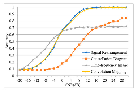
Figure 5. The performance of the radio–image transformer (RIT) methods on dataset Sig1024, compared with the constellation diagram method and time–frequency image method.

Table 3. Comparison of the overall classification accuracy of the four methods. The dataset is Sig1024.

Methods	SRM	Constellation	Time–Frequency	CMM
ResNet18	65.99%	40.27%	55.79%	65.49%

5.2.3. Performance of Different ImageNet Models

Using the convolution mapping method, we compare the classification accuracy obtained by using different ImageNet classification models on dataset Sig1024, including the typical convolutional neural networks ResNet18, ResNet101, VGG16 and DenseNet121, as well as the lightweight models MobileNet, ShuffleNet and MNASNet. Table 4 shows the overall classification accuracy of these methods and Figure 6 shows the classification accuracy of these models under different SNRs. We can see that except for the relatively low classification accuracy of the MNASNet model, the classification results of the other models have little difference. Among them, DenseNet121 has the highest overall accuracy.

Table 4. Comparison of the overall classification accuracy of different models. The convolution mapping method was adopted.

CNNs	ResNet18	ResNet101	VGG16_bn
Accuracy	65.49%	66.47%	65.43%
DenseNet121	MobileNet_V2	ShuffleNet_v2_x1_0	MNASNet1_0
67.47%	66.63%	65.06%	49.27%

Figure 6. Comparison of the performance of different ImageNet classification network models. The convolution mapping method was adopted.

5.2.4. Performance with Different Sampling Rates

We test the performance of our method on dataset Sig1024_2 with different sampling rates. We use CMM and MobileNet_V2 model and the classification accuracy of each SNR is shown in the Figure 7. We can see that in this case, our method still has good classification performance. This shows that the method can be used to classify radio signals with different sampling rates as long as the model has been trained with signal samples with these sampling rates.

Figure 7. Classification accuracy of each SNR of dataset Sig1024_2 with 2 different sampling rates.

5.2.5. Performance with Real Measured Data

We also verify the effectiveness of our method by using real measured dataset RealSig to test the MobileNet_V2 model trained in the third experiment. Figure 8 shows the classification accuracy of each SNR. It is clear that the model we trained on the simulation dataset Sig1024 with CMM and MobileNet_V2 also has good classification accuracy for the real measured 16QAM and 64QAM signals.

Figure 8. Classification accuracy of each SNR of the real dataset RealSig. The classification method is CMM and the CNN model used is MobileNet_V2.

To further improve the performance, we add the training set in dataset RealSig to fine-tune the model MobileNet_V2 trained with dataset Sig1024 with a learning rate of 0.00001, and then test the model’s classification performance on the test set. The classification accuracy of each SNR is shown in Figure 9. We can see that the classification accuracy can be improved to nearly 100% at high SNR.

Figure 9. Classification accuracy of each SNR of the real dataset RealSig. The MobileNet_V2 model is fine-tuned.

5.2.6. Performance of OFDM Signal Classification

Finally, we carry out experiments on dataset OFDMSig to verify the effectiveness of our method, using CMM and MobileNet_V2. The classification result is shown in Figure 10. It can be seen that our method also has a good classification performance on the dataset OFDMSig, achieving a classification accuracy of 100% at the high SNR.

Figure 10. Classification accuracy of each SNR of dataset OFDMSig.

6. Conclusions

In this paper, we have proposed a RIT that transforms radio signals into images, and then the existing ImageNet classification network models are utilized to realize radio modulation classification, thus building a bridge between radio modulation classification and ImageNet classification. The contribution of this paper is to transform the signal modulation classification problem into the image classification problem by the proposed RIT, enabling signal classification using ImageNet models from the image classification domain. Experiments have shown that the performance of this method is better than those of the constellation diagram method and time–frequency image method. The performance comparison of different ImageNet classification network models shows that except for MNASNet1_0, the other six models have similar performance, which indicates that this method has relatively loose requirements for ImageNet classification network models. Furthermore, the experimental results show that our method has good classification performance for signal datasets with different sampling rates and our method can also handle OFDM signals and real measured signal data well. The method in this paper establishes a relationship between radio modulation classification and ImageNet image classification, two seemingly unrelated tasks, and verifies the cross-domain transfer ability of ImageNet classification network models. In our future work, we will consider applying a similar RIT to other radio signal classification tasks, such as interference classification, coding recognition, and protocol identification.

References

- Haykin, S.; Setoodeh, P. Cognitive Radio Networks: The Spectrum Supply Chain Paradigm. IEEE Trans. Cogn. Commun. Netw. 2015, 1, 3–28. [Google Scholar] [CrossRef]
- Yucek, T.; Arslan, H. A survey of spectrum sensing algorithms for cognitive radio applications. IEEE Commun. Surv. Tutor. 2009, 11, 116–130. [Google Scholar] [CrossRef]
- Zheng, S.; Chen, S.; Yang, L.; Zhu, J.; Luo, Z.; Hu, J.; Yang, X. Big Data Processing Architecture for Radio Signals Empowered by Deep Learning: Concept, Experiment, Applications and Challenges. IEEE Access 2018, 6, 55907–55922. [Google Scholar] [CrossRef]
- Rajendran, S.; Calvo-Palomino, R.; Fuchs, M.; Van den Bergh, B.; Cordobes, H.; Giustiniano, D.; Pollin, S.; Lenders, V. Electrosense: Open and Big Spectrum Data. IEEE Commun. Mag. 2018, 56, 210–217. [Google Scholar] [CrossRef]
- Ulversoy, T. Software Defined Radio: Challenges and Opportunities. IEEE Commun. Surv. Tutor. 2010, 12, 531–550. [Google Scholar] [CrossRef]
- Emam, A.; Shalaby, M.; Aboelazm, M.A.; Bakr, H.E.A.; Mansour, H.A.A. A Comparative Study between CNN, LSTM, and CLDNN Models in the Context of Radio Modulation Classification. In Proceedings of the 2020 12th International Conference on Electrical Engineering (ICEENG), Cairo, Egypt, 7–9 July 2020. [Google Scholar]
- Kim, S.H.; Kim, C.Y.; Yoo, S.H.; Kim, D.-S. Design of Deep Learning Model for Automatic Modulation Classification in Cognitive Radio Network. J. Korean Inst. Commun. Inf. Ences. 2020, 45, 1364–1372. [Google Scholar]
- Zhu, Z.; Nandi, A.K. Automatic Modulation Classification: Principles, Algorithms and Applications; John Wiley & Sons: Hoboken, NJ, USA, 2015; ISBN 9781118906491. [Google Scholar]
- Dobre, O.A.; Abdi, A.; Bar-Ness, Y.; Su, W. Survey of automatic modulation classification techniques: Classical approaches and new trends. IET Commun. 2007, 1, 137–156. [Google Scholar] [CrossRef]
- Swami, A.; Sadler, B.M. Hierarchical digital modulation classification using cumulants. IEEE Trans. Commun. 2000, 48, 416–429. [Google Scholar] [CrossRef]
- Soliman, S.S.; Hsue, S.-Z. Signal classification using statistical moments. IEEE Trans. Commun. 1992, 40, 908–916. [Google Scholar] [CrossRef]
- Grimaldi, D.; Rapuano, S.; Vito, L.D. An Automatic Digital Modulation Classifier for Measurement on Telecommunication Networks. IEEE Trans. Instrum. Meas. 2007, 56, 1711–1720. [Google Scholar] [CrossRef]
- Majhi, S.; Gupta, R.; Xiang, W.; Glisic, S. Hierarchical Hypothesis and Feature-Based Blind Modulation Classification for Linearly Modulated Signals. IEEE Trans. Veh. Technol. 2017, 66, 11057–11069. [Google Scholar] [CrossRef]
- LeCun, Y.; Bengio, Y.; Hinton, G. Deep learning. Nature 2015, 521, 436–444. [Google Scholar] [CrossRef] [PubMed]
- Deng, J.; Dong, W.; Socher, R.; Li, L.; Li, K.; Li, F.-F. ImageNet: A large-scale hierarchical image database. In Proceedings of the 2009 IEEE Conference on Computer Vision and Pattern Recognition, Miami, FL, USA, 20–25 June 2009; pp. 248–255. [Google Scholar]
- O’Shea, T.J.; Corgan, J.; Clancy, T.C. Convolutional radio modulation recognition networks. Proc. Int. Conf. Eng. Appl. Neural Netw. 2016, 629, 213–226. [Google Scholar]
- O’Shea, T.J.; Roy, T.; Clancy, T.C. Over-the-Air Deep Learning Based Radio Signal Classification. IEEE J. Sel. Top. Signal Process. 2018, 12, 168–179. [Google Scholar] [CrossRef]
- Zheng, S.; Qi, P.; Chen, S.; Yang, X. Fusion Methods for CNN-Based Automatic Modulation Classification. IEEE Access 2019, 7, 66496–66504. [Google Scholar] [CrossRef]
- Rajendran, S.; Meert, W.; Giustiniano, D.; Lenders, V.; Pollin, S. Deep Learning Models for Wireless Signal Classification With Distributed Low-Cost Spectrum Sensors. IEEE Trans. Cogn. Commun. Netw. 2018, 4, 433–445. [Google Scholar] [CrossRef]
- Peng, S.; Jiang, H.; Wang, H.; Alwageed, H.; Zhou, Y.; Sebdani, M.M.; Yao, Y. Modulation Classification Based on Signal Constellation Diagrams and Deep Learning. IEEE Trans. Neural Netw. Learn. Syst. 2019, 30, 718–727. [Google Scholar] [CrossRef]
- Akeret, J.; Chang, C.; Lucchi, A.; Refregier, A. Radio frequency interference mitigation using deep convolutional neural networks. Astron. Comput. 2017, 18, 35–39. [Google Scholar] [CrossRef]
- Czech, D.; Mishra, A.; Inggs, M. A CNN and LSTM-based approach to classifying transient radio frequency interference. Astron. Comput. 2018, 25, 52–57. [Google Scholar] [CrossRef]
- Selim, A.; Paisana, F.; Arokkiam, J.A.; Zhang, Y.; Doyle, L.; DaSilva, L.A. Spectrum Monitoring for Radar Bands Using Deep Convolutional Neural Networks. In Proceedings of the GLOBECOM 2017—2017 IEEE Global Communications Conference, Singapore, 4–8 December 2017; pp. 1–6. [Google Scholar]
- Krizhevsky, A.; Sutskever, I.; Hinton, G. ImageNet classification with deep convolutional neural networks. Commun. ACM 2017, 60, 84–90. [Google Scholar] [CrossRef]
- Zeiler, M.D.; Fergus, R. Visualizing and Understanding Convolutional Networks. Lect. Notes Comput. Sci. (Incl. Subser. Lect. Notes Artif. Intell. Lect. Notes Bioinform.) 2014, 8689, 818–833. [Google Scholar]
- Simonyan, K.; Zisserman, A. Very Deep Convolutional Networks for Large-Scale Image Recognition. arXiv 2014, arXiv:1409.1556. [Google Scholar]
- Christian, S.; Wei, L.; Yang, J.; Pierre, S.; Scott, R.; Dragomir, A.; Dumitru, E.; Vincent, V.; Andrew, R. Going deeper with convolutions. In Proceedings of the IEEE Conference on Computer Vision and Pattern Recognition (CVPR), Boston, MA, USA, 7–12 June 2015; pp. 1–9. [Google Scholar]
- He, K.; Zhang, X.; Ren, S.; Sun, J. Deep Residual Learning for Image Recognition. In Proceedings of the IEEE Conference on Computer Vision and Pattern Recognition (CVPR), Las Vegas, NV, USA, 27–30 June 2016; pp. 770–778. [Google Scholar]
- Iandola, F.; Han, S.; Moskewicz, M.W.; Ashraf, K.; Dally, W.J.; Keutzer, K. SqueezeNet: AlexNet-level accuracy with 50x fewer parameters and <0.5 MB model size. arXiv 2017, arXiv:1602.07360. [Google Scholar]
- Chollet, F. Xception: Deep Learning with Depthwise Separable Convolutions. In Proceedings of the IEEE Conference on Computer Vision and Pattern Recognition (CVPR), Honolulu, HI, USA, 21–26 July 2017; pp. 1800–1807. [Google Scholar]
- Howard, A.; Zhu, M.; Chen, B.; Kalenichenko, D.; Wang, W.; Weyand, T.; Andreetto, M.; Adam, H. MobileNets: Efficient Convolutional Neural Networks for Mobile Vision Applications. arXiv 2017, arXiv:1704.04861. [Google Scholar]
- Zhang, X.; Zhou, X.; Lin, M.; Sun, J. ShuffleNet: An Extremely Efficient Convolutional Neural Network for Mobile Devices. In Proceedings of the IEEE/CVF Conference on Computer Vision and Pattern Recognition, Salt Lake City, UT, USA, 18–23 June 2018; pp. 6848–6856. [Google Scholar]
- Kingma, D.P.; Ba, J. Adam: A Method for Stochastic Optimization. arXiv 2014, arXiv:1412.6980. [Google Scholar]
© 2020 by the authors. Licensee MDPI, Basel, Switzerland. This article is an open access article distributed under the terms and conditions of the Creative Commons Attribution (CC BY) license (http://creativecommons.org/licenses/by/4.0/).