Article

Random Number Generator with Long-Range Dependence and Multifractal Behavior Based on Memristor

1
Electronic Engineering Department, Universidad Distrital Francisco José de Caldas, Bogotá 110221, Colombia
2
Electrical Engineering Department, Universidad Distrital Francisco José de Caldas, Bogotá 111711, Colombia
*
Author to whom correspondence should be addressed.
Electronics 2020, 9(10), 1607; https://doi.org/10.3390/electronics9101607
Submission received: 13 August 2020 / Revised: 15 September 2020 / Accepted: 17 September 2020 / Published: 1 October 2020
(This article belongs to the Special Issue Fractional-Order Circuits & Systems Design and Applications)

Abstract

:
Random number generators are used in areas such as encryption and system modeling, where some of these exhibit fractal behaviors. For this reason, it is interesting to make use of the memristor characteristics for the random number generation. Accordingly, the objective of this article is to evaluate the performance of a chaotic memristive system as a random number generator with fractal behavior and long-range dependence. To achieve the above, modeling memristor and its corresponding chaotic systems is performed, from which a random number generator is constructed. Subsequently, the Hurst parameter for the detection of long-range dependence is estimated and a fractal analysis of the synthesized data is performed. Finally, a comparison between the model proposed in the research and the β-MWM algorithm is made. The results obtained show that the data synthesized from the proposed generator have a variable Hurst parameter and both monofractal and multifractal behavior. The main contribution of this research is the proposal of a new model for the synthesis of traces with long-range dependence and fractal behavior based on the non-linearity of the memristor.

1. Introduction

Random number generators (RNGs) are currently used to encrypt information and model natural processes. In the encryption area, RNGs allow to encoding information that is transmitted from one point to another without running the risk of being deciphered by an external agent. To achieve this, complex encryption processes are required to decipher the information only through the encryption key. In most cases, this encryption key is a combination of a data sequence with the information to be transmitted [1]. These sequences must be sufficiently long and random enough, in addition to presenting independence between the generated values [2]. For the generation of independent random numbers, the inverse transformation method can be used: a uniformly distributed random number is generated, with parameters 0 and 1, and it is evaluated in the desired quantile function (the inverse of the cumulative function). Now, although the inverse transformation method solves the problem of the type of distribution, it only allows the generation of independent random numbers and, consequently, it is not suitable for modeling natural processes that are highly correlated and that show dependencies between the different scales; for example: detection of climate zones [3], market behavior [4] and video traffic in Moving Picture Experts Group 4 (MPEG-4) [5].
It has been found that some algorithms for the random traces generation show similar behavior to natural processes, especially in traffic networks [3,4,5,6,7]. Strict self-similarity is very restrictive in adequately characterizing many types of signals that exhibit long range dependence (LRD). For example, Ethernet traffic [8] has LRD, but shows short-term correlations and scale behavior inconsistent with strict or monofractal self-similarity, in which a single parameter: Hurst’s, is sufficient to characterize the whole set of data [9]. Furthermore, the scaling behavior of the moments, when the Ethernet traffic is aggregated, is a non-linear function of the order of the moments [10]. When the traffic exhibits such characteristics, it is considered multifractal. Multifractal signals are positive measures or distributions that possess self-similarity with inhomogeneous scalability [10]. Multifractal behavior has been detected in the traffic: transmission control protocol (TCP) [9], wide area network (WAN) Internet [11], variable bit rate (VBR) video [12] and MPEG-4 video [5], among others.
An important contribution to this area is the multifractal wavelet model (MWM), by Riedi et al. [10]. The MWM uses a multiplicative structure based on the Haar wavelet transform to synthesize N samples of a traffic trace with computational complexity O ( N ) . The model captures not only the power spectrum (hence the LRD), but also the higher order statistics. The MWM has been explored in [10] for the generation of discrete multifractal sequences, with success, and has been applied by two of the authors in the area of cognitive radio [13].
Despite the advantages that MWM offers, it is desired to propose a method that not only generates discrete multifractal sequences, and that therefore can be applied to other areas, such as bioengineering, in which monofractality has been detected [14]. Specifically, the authors are interested in developing a synthetic electrocardiographic (ECG) signal generator [15], with LRD, in which the cardiac rhythm values are fed by the monofractal RNG and thus the dependence between the consecutive cardiac rhythms is guaranteed. The proposed generator would facilitate the correct evaluation of the algorithms that help to detect changes in cardiac rhythm (as occurs in arrhythmias), while allowing us to compare the model with real hardware.
Additionally, MWM presents another disadvantage, when it is desired to transfer its implementation to hardware. The MWM requires the generation of the complete data set, of length N = 2 n , with n 20 , when it is desired to specify the sample multifractal characteristics, within acceptable confidence intervals [16]. The memory waste is unacceptable when it is evidenced that to get only m random numbers, it is required to throw away the remaining 2 n m . Therefore, this article presents the search and characterization of a versatile random number generator (RNG) that, unlike the inverse transformation method, presents LRD; and that, unlike MWM, exhibits both monofractal and multifractal behavior. Additionally, it is desired to solve the problem of inefficiency for the generation of a few random numbers.
To solve the last, we must focus on the chaotic dynamical systems: the description in difference equations could generate the next sample, based on the current sample and the dynamics of the non-linear system. Furthermore, for LRD to occur, the system would have to be chaotic, since self-similarity is related to it [17]. It is in this sense that the memristor is presented as the suitable candidate to be the core of a random number generator with LRD (this research shows evidence that validates this hypothesis, although other chaotic systems are not ruled out, which also allow it).
In 1971, Chua [18] proposed the memristor as a non-linear device with two terminals that allows to directly relate the flux and charge variables of the faraday’s law of induction. In 2010, Muthuswamy and Chua [19] designed and implemented a chaotic circuit using the memristor, evidencing the application of this as a RNGs. Although the use of the memristor as a random number generator is not new, the possibility of using it as a source of Hardware random-number generator (since it is a non-linear device sensitive to initial conditions) in conjunction with a versatile structure that allows adjusting the Hurst parameter, choose monofractality/multifractality, or even adjust the width of the multifractal spectrum, has not been evidenced in the literature reviewed to date. In this article, the existence of the monofractal/multifractal behavior of a memristor-based RNG is detected, it is shown that its characteristics can be modified and it is shown what could be done to achieve it.
The rest of the article is structured as follows. Section 2 mentions some of the works related to the topic of RNGs, long-range dependence and multifractal analysis. Section 3 describes the methodology used. Subsequently, Section 4 presents the results achieved in the investigation. And finally, Section 5 presents the conclusions and future work.

2. Related Work

In the field of chaotic systems, several works describing different memory circuits and functions have been published. In principle, Cruz and Chua [20] mathematically develop a chaotic system using a device which was called the Chua diode. Subsequently, Muthuswamy and Chua [19] generated another chaotic oscillator using a memristor. From this, several authors have made modifications both in the memory function memconductance and in the circuit for specific applications. For example, in [21,22] new functions are implemented to generate chaotic systems. In 2016 and 2017 new circuits were proposed for encryption and decryption of images and texts [23].
Through the previous investigations, several RNGs have been built. Some of these proposals can be studied in [24,25], where RNGs are implemented based on a chaotic signal emulated by an FPGA and sampling the signal presented in [19]. The result of both articles is the implementation of a system capable of approving the National Institute of Standards and Technology (NIST) test bench for its application in computer security systems.
Other generators are exposed by Melgarejo and Piraján [26], who propose a random number generator from a noisy signal emanating from a Zener diode, obtaining a generator with normal or uniform distribution and with particular statistical characteristics; and Li et al. [27], who built a RNGs based on a chaotic signal emanated by a laser, with the possibility of generating random bits every 10 Gb/s.
On the other hand, Leland et al. [7] observed the self-similar nature of Ethernet traffic, showing that such traffic is statistically self-similar and showing that the degree of self-similarity is an indication of traffic variability, estimated in terms of the Hurst parameter. What was stated by [7] allowed to conclude that the models used until that moment were incapable of capturing this property, opening the way to the characterization and modeling of modern traffic. This need led to the study of fractal traffic through the Wavelet transform [18,19,20,21,28,29,30,31]. For this reason, Riedi et al. [10] proposed a wavelet multifractal model (WMM) which characterizes and synthesizes positive data with long-range dependence (LRD) and Tuberquia et al. [32] made an algorithm to generate multifractal time series with Hurst parameter and multifractal spectrum width, sample and adjustable.
As evidenced in the previous paragraphs, there are no works that generate random numbers based on a chaotic system with LRD and that exhibit fractal behavior. Related investigations allow the generation of random numbers without performing the fractal analysis of the synthesized traces. In this research a proposal of a model that starts from a physical signal to generate traces with said behaviors is developed.

3. Materials and Methods

The scheme of Figure 1 represents the methodology used in this investigation. Initially, the memristor device is introduced, which allows it (from its non-linear behavior) to generate the chaotic systems implemented as physical signals for the proposed RNG model, which synthesizes the traces of data to be analyzed. Subsequently, the NIST test bench is used to measure the degree of randomness of the synthesized data [7]. Some sequences were estimated with the Hurst parameter (H) for the detection of LRD from two tools: the variance-time diagram (VT) and the log-scale diagram (LD). The first calculates the moments of aggregation and the autocovariance of the process X[k] [33]. The second computes the average of the detail coefficients of the discrete wavelet transform [25,26]. If these traces have long-range dependence, they can be classified as single—or multifractal with multiscale (MD) and linear multiscale (LMD) diagrams [25,27]. Similarly, the multifractal spectrum (MS) allows analyzing fractal processes from the Legendre transform [10], providing information on the data trace, such as its fractal dimension, spectrum width and information dimension, among others [34,35,36,37].

3.1. Memristor

In the decade of the 60s research was started on a device that would represent the link lost in the relation of the four circuital variables exposed in the deduction of Faraday’s law of induction: voltage v, current i, flux ϕ and charge q [38]. It was then that Widrow [39] developed a new device called a memistor. This is a three-terminal device, for which the conductance between two of its terminals is controlled by the time integral of the current at the third terminal, and its resistance by the charge. Chua [18], who is considered the father of non-linear circuits, predicted the existence of a missing element that would relate the charge to the flux. To this element Professor Chua called it memristor. The memristor is a nonlinear two terminal device that directly relates flux and charge. There are two models of memristor: one controlled by charge and another controlled by flux, which are described in Equations (1) and (2).
charge controlled   Memristor { V ( t ) = M ( q ( t ) ) i ( t ) [ V ] M ( q ) = d φ ( q ) / d q   [ Ω ] p ( t ) = M ( q ( t ) ) i 2 ( t ) [ W ]
flux controlled   Memristor { i ( t ) = W ( φ ( t ) ) v ( t ) [ A ] W ( φ ) = d q ( φ ) / d φ   [ S ] p ( t ) = W ( φ ( t ) ) v 2 ( t ) [ W ]
Chua [18] named the function M(q(t)) as the memristive and W(φ(t)) as the memductance. For a device to be considered memristor, it must comply with the following characteristics [31,32]:
  • The device must exhibit a pinched hysteresis loop in the voltage-current plane for some period of excitation signal.
  • The area of the pinched hysteresis lobe should decrease monotonically with excitations of increments in frequency.
  • The pinched hysteresis loop must shrink to a simple function value when the frequency tends to infinity.
Memristors have a wide range of applications: memristor based on RRAM memories [40,41,42], sinusoidal oscillators [33,34,35,43], random number generators [44,45], programmable analog circuits [45], adaptive filters [37,38,46,47], neuromorphic circuits [48], and chaotic systems [7,11,12].

3.2. Chaotic Systems

In this section, the chaotic systems that synthesize the input signals for the random number generator, based on memristor as a device that provides the non-linearity, are presented. Each system displays the phase diagram of two electrical variables measured in their respective electrical circuit, in addition to presenting the system of equations that describe it.

3.2.1. System 1

One of the first circuits proposed by Cruz and Chua [20] as a generator of chaotic systems is shown in Figure 2a, with the phase diagram of Figure 2b. Cruz and Chua [20] used the Chua diode for this purpose, which emulates a linear piecewise function in the form of a current that depends on the potential differential between its two terminals. The mathematical development of Figure 2a is shown in Equation (3).
{ C 2   d d t V C 2 = V C 1 R V C 2 R i D ( V C 2 ) C 1   d d t V C 1 = V C 2 R V C 1 R + i L L d d t i L = V C 1

3.2.2. System 2

Chaotic generators have been used for the encryption and decryption of information. Yang et al. [23] designed and implemented a chaotic circuit (Figure 3a) in which the memristive is a piecewise linear function, similar to the one exposed in the Chua diode. Yang et al. [23] describe the steps to encrypt and decrypt text and images. The structure of the circuit is presented in Figure 3b, which is generated by Equation (4).
{ C 2 d d t V C 2 = i L V C 2 W ( φ ) C 1 d d t V C 1 = G V C 1 i L L d d t i L = V C 1 V C 2 d d t φ = V C 2

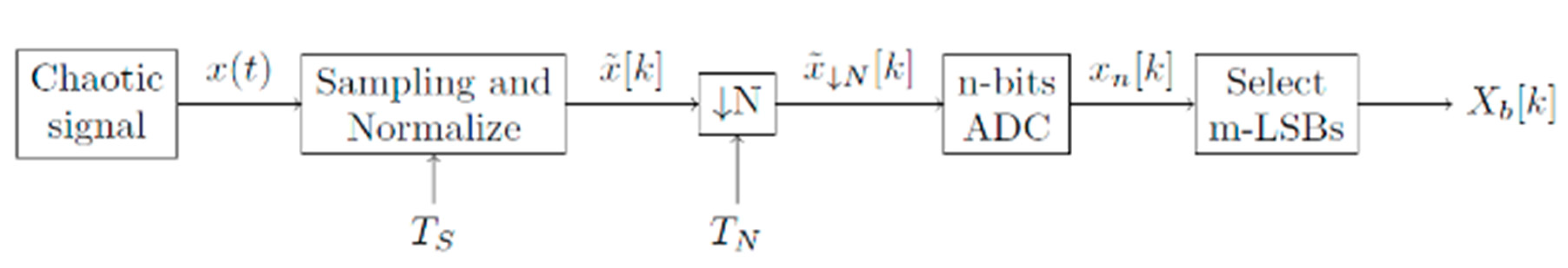
3.3. Random Number Generator (RNG)

Below the procedure for generating a sequence of random numbers from a chaotic input signal is explained. The starting point lies in the model presented by Li et al. [27] (Figure 4), to which modifications have been made including the proposal of Corinto et al. [25] to synthesize data with greater randomness. The degree of randomness is measured with the NIST test bench.
The block diagram of Figure 4 shows the process for an RNG dependent on a chaotic signal (for example, emitted by a laser beam) [27]. In this investigation the chaotic signal will be generated by the two systems presented previously.
The resolution of the analog to digital converter (ADC) block depends on the n-bits of the converter, allowing to distinguish values closer to each other with a larger number of bits. This suggests that at a high sampling rate, an ADC with low resolution will allow the conversion of consecutive equal data, decreasing the randomness of the generator. Therefore, it is necessary to add an intermediate block that reduces the sampling rate depending on the number of bits of the converter to eliminate unnecessary information from the chaotic signal sampled. A normalization block is also added in order to decrease the sampling rate of the multitasking processor. The calculation of this rate is shown in Equations (5) and (6).
T N = ( max X k min X k ) T s ( 2 n 1 ) max | X [ k ] X [ k 1 ] |
N = [TN/TS]
The intention of the Equation (5) is to find the biggest difference between consecutive data of the sampled signal and normalized input, in order to reduce the sampling rate using the limit values of the signal and this difference, without neglecting the number of bits of the ADC. This value must be calculated a priori and reduced to a constant. The modifications are presented in Figure 5.
In order to grant more randomness to the RNG, inspired by [25], the generator combines the first three state variables of each chaotic system, sampled with the process of Figure 5 and generates a unique binary sequence. Following, a b-bits DAC and another normalization block are inserted at the output to deliver discrete numbers in a wider range to the binary (W[K] ∈ [0, 1]). Figure 4 is extended to Figure 6 with these modifications.

3.4. NIST Tests

The NIST test bench, described in [49,50] consists of fifteen (15) statistical tests to prove the randomness of binary (arbitrarily long) sequences produced by random or pseudo-random generators based on software or hardware, to be implemented in applications of information encryption. The data synthesized by the generator is subjected to these tests in order to discard traces with low approval rate. The tests that the bank performs are:
  • The frequency (monobit) test;
  • Frequency test within a block;
  • The cumulative sums (cusums) test;
  • The runs test;
  • Tests for the longest-run-of-ones in a block;
  • The binary matrix rank test;
  • The discrete Fourier transform (spectral) test;
  • The overlapping template matching test;
  • Maurer’s “universal statistical” test;
  • The approximate entropy test;
  • The serial test;
  • The linear complexity test;
  • The random excursions test;
  • The random excursions variant test;
  • The non-overlapping template matching test.
Each test assumes that the data is random. This hypothesis is rejected if the result of the p-value (mathematical result of each test) is lower than a constant α . By default α = 0.01. indicating that only an error equal to or less than 1% is accepted. The NIST test bench is rigorous because its focus is on sequences used for information encryption. The documentation and source files to execute them can be downloaded [51].
Below the procedure for generating a sequence of random numbers from a chaotic input signal is explained. The starting point lies in the model presented by Li et al. [27] (Figure 4), to which modifications have been made including the proposal of Corinto et al. [25] to synthesize data with greater randomness. The degree of randomness is measured with the NIST test bench.

3.5. Diagram Variance-Time

In this section the procedure to detect the LRD from the estimation of the Hurst parameter by means of the VT diagram is outlined. Then an example trace is exposed and the Hurst parameter is estimated with this tool. For a stochastic discrete time process X[k], kN its aggregate process X(m) is defined, with an aggregation level m, as shown in Equation (7) [33]:
X ( m ) [ i ] = 1 m k = m ( i 1 ) + 1 m i x [ k ]
If the autocovariance function of X is asymptotically self-similar of second order (Equation (8)):
lim m y m [ k ] = σ x 2 2 [ ( k + 1 ) 2 H 2 k 2 H + ( k 1 ) 2 H ]
If γ is the autocovariance function and the Hurst parameter H is between 0.5 < H < 1, it is said that the stochastic process X has long-range dependence. This shows a relationship of stochastic process data, since for values of H < 0.5, the autocovariance of X[k] becomes close to zero. While for H = 1, the autocovariance is equal to the variance, thus presenting a particular case [33]. Furthermore, if the process X[k] is exact or asymptotically self-similar, the sample variance of the aggregate process is found from Equation (9).
S X ( m ) 2 = σ X 2 m 2 H 2
Now, when applying the logarithm function on both sides of the Equation (9), get Equation (10):
log S X ( m ) 2 = log σ x 2 + ( 2 H 2 ) log m
Thus, if it is assumed in a graph that y = log S2x (m) and x = log (m), the Hurst parameter could be estimated by means of a linear regression. In the literature this graph is known as the variance-time diagram [36].
Sheluhin et al. [36] show the performance of the VT diagram and explain that it is a tool used as a diagnosis, since it is biased and, in addition, the bias increases with the growth of H. On the other hand, the use of the wavelet transform for parameter estimation of Hurst is not parametric and the estimator of its variance is not biased [33]. For this reason, tools such as the log-scale diagram are used.

3.6. Diagram Log-Scale

In this section the mathematical model for the construction of the LD is presented. The basis of this tool is the discrete wavelet decomposition of the stochastic process X[k], calculating the detail coefficients by means of a filter bank with multiple sampling rates.
The continuous wavelet decomposition (CWT) of a signal X(t) is a linear transformation defined by Equation (11) [34].
T x ( a , b ) X ( t ) Ψ ( ( t b ) / a ) d t , a , b
A fundamental characteristic of the CWT is its redundancy, since neighboring coefficients share information about X(t). To reduce this redundancy, the discrete wavelet transform is introduced into the Equation (12) [36]:
d X ( j ,   k ) = T X ( 2 j ,   2 j k ) , j , k +
Being dX(j,k) the detail coefficients of the wavelet transform. The respective scale function is obtained with a bank of multi-tasking filters [25,26]. A temporal estimator has a small variance when there is a lack of correlation between the detail coefficients. This can be estimated for the process dX(j,●) by Equation (13) [26,27].
μ j = 1 n j k = 1 n j d X ( j ,   k ) 2
where nj is the number of detail coefficients in the octave j and µj ≈ E [|dx(j,k)|2]. Since the second moment of the detail coefficients follows a power law with exponent 2H − 1, it is possible to estimate the Hurst parameter, using the estimator (Equation (14)) [36]:
y j = log 2 μ l = ( 2 H 1 ) j + log 2 C
The graph of j versus y j is nown as the log-scale diagram [35]. The value of H is an approximation that depends on the amount of detail coefficients used and the number of octaves used in the linear regression. Taking the plot exposed in [52], in Figure 7 shows the series of times with LRD (Figure 7a) and the estimation of the Hurst parameter with the LD between octaves 3 and 14 (Figure 7b).

3.7. Multiscale Diagram and Linear Multiscale

Now the MD and LMD tools used as the first approach to the multifractal analysis are shown, explaining in a rough way the mathematical basis of each diagram and illustrating the implementation of each tool with two traces as an example. The estimator of order q of a process dx(j,●) show in Equation (15) as an extended concept of the estimator of the Equation (13) to higher order moments [25,27].
μ j q = 1 n j k = 1 n j d X ( j ,   k ) q
For processes with LRD, the estimator of Equation (15) follows the law of powers shown in Equation (16) [34].
μ j q E [ d X ( j ,   k ) q ] = C q 2 j ( ζ ( q ) q / 2 )  
where C q is a function that depends on the order of the estimator and ζ(q) is a function that allows to distinguish between monofractal and multifractal processes. If the estimator of Equation (13) is equal to that of Equation (15), the expression ζ(q) = qH is satisfied, with which it is deduced that said process is monofractal [36]. Thus, in a similar way to the analysis carried out in Equation (10) and Equation (14), the multiscale diagram is obtained when performing the graph of the Equation (17).
ζ ( q ) = α q + q / 2
where αq can be computed by Equation (18).
log 2 μ j q = log 2 ( ( 1 / n j ) k = 1 n j d X ( j ,   k ) q ) α q j + log 2 C q
Two processes with LRD are analyzed: interarrival times of BCpAu89 trace with multifractal behavior and Fractional gaussian noise with monofractal. For q > 0 the time series with multifractal is convex, but empirically determining this fact is complex. For this reason, the linear multiscale diagram described by Equation (19).
H ( q ) =   α q / q + 1 / 2
If the process with LRD presents monofractal behavior, the Equation (19) satisfies the expression h(q) = H and therefore, this process presents the same parameter of Hurst in all orders.

3.8. Multifractal Spectrum

As a last tool, the Legendre transform is introduced as the main foundation for the built of the multifractal spectrum. The process of transforming the mass exponents to their local dimension is briefly exposed, allowing to differentiate multifractal sequences of monofractals.
By means of the Legendre transform, the multifractality can be analyzed in a process with LRD, for which it is necessary to know the exponents of mass τ(q) (Equation (20)).
τ ( q ) = q H ( q ) 1
From Equation (20) the singular exponent α(q) is defined (Equation (21)).
α ( q ) = d d q τ ( q )
At this point, the Legendre transform defined by the Equation (22), which represents the local dimension of the multifractal set [53].
f ( α ( q ) ) = q α ( q ) τ ( q )
Finally, the multifractal spectrum is obtained by plotting the singular exponent versus the local dimension of the multifractal set. The result is a long concave bow down where the difference between the minimum of α(q) and its maximum is called the multifractal spectrum width [54] for multifractional processes and a local point for monofractal processing. For a more detailed explanation, consult [32].
In principle, the exponents of mass τ(q) are calculated to find the singular exponent α(q) and after, the Legendre transform of the time series. Finally, the multifractal behavior of the traces is observed, concluding the multifractal nature of the trace Interarrival times of BCpAu89 and the monofractal nature of Fractional gaussian noise.

3.9. Multiplicative Cascades

The multifractal wavelet model (MWM) proposed by [10] provides an algorithm for the synthesis of data with LRD by means of a binomial conservative cascade of computational complexity O(N). This algorithm is used as a reference point in the investigation. Riedi et al. [10] establishes the possibility of generating traces of multifractal data with LRD, assuming that the multiplying coefficients p and p − 1 must be random variables, identically distributed, with a mean of 0.5, that take values in the interval [0, 1] and have a beta probability distribution defined in Equation (23) [55].
f X ( x ; α ,   β ) = { Γ ( α + β ) / Γ ( α ) Γ ( β )   x α 1 ( 1 x ) β 1 0 0 < x < 1 α , β > 0 x ( 0 , 1 )
When the parameters α and β are equal (Equation (24)), the density function beta is symmetric with respect to 0.5 and therefore, the average takes the value of 0.5. Riedi et al. [10] shows that using a symmetric beta density function as expressed in Equation (24) for the multipliers of the Wavelet coefficients (called the β -MWM model) it is possible to control the Hurst parameter when modifying the β parameter of the multipliers. The relationship proposed by Riedi et al. [10] is shown in Equation (25).
f X ( x ; β ,   β ) = { Γ ( 2 β ) / Γ ( β ) 2   x β 1 ( 1 x ) β 1 0 0 < x < 1 β > 0 x ( 0 , 1 )
β = ( 2 2 H 1 1 ) / ( 2 2 2 H 1 )
An example of implementation of the β-MWM algorithm is shown in Figure 8 for a data length 220, condition of U0,0 = 100 and Hurst parameter H = 0.9.
In Figure 9a–c the MD, LMD and MS are exposed, respectively. With these diagrams, the multifractal behavior of the trace generated by the β-MWM algorithm is affirmed. It should be noted that the width of the spectrum can be modified with different values of H .
The estimate of the Hurst parameter for this trace is shown in Figure 10a,b. Note the estimation of the Hurst parameter with respect to the one introduced in the algorithm.

4. Results

The results show the combinations of the RNG used to synthesize the different random sequences submitted to the NIST tests. Then, the result of the tools applied to the data for the detection of LRD and multifractal analysis is displayed. Finally, a brief comparison is made between the proposed generator and the β-MWM algorithm.

4.1. Random Number Generator

Using the RNG shown in Figure 6 for the chaotic signals of the six (6) systems, random sequences of length 1 × 10⁶ were synthesized by varying the parameters of the generator, such as the quantity of n-bits used in the ADC, the quantity m-LSBs taken from the ADC and the number of b-bits used in the DAC, where b = 0 is the output of the RNG a purely binary data sequence (the DAC is not used). When synthesizing the different sequences, it was shown that some combinations had a deterministic behavior or LRD was not detected, where it was necessary to implement the threshold function (Equation (26)) to the traces generated with b ≠ 0, because the NIST tests are only implemented for binary data.
f h ( x ) = { 0   P a r a   x < 0.5 1   P a r a   x 0.5
Each sequence was submitted to the first fourteen NIST tests, with parameters chosen according to Table 1 (in those tests that needed an external parameter).
From Table 2 and Table 3, the p-value computation is shown for each combination defined by each NIST test. The default value of α is taken to discriminate the sequences, with p-value < α a failed test. The possible causes of a p-value < α are due to the correlated data or that the threshold function does not adapt to the data. It is observed that the tests with the lowest approval rate are: frequency test within a block, the discrete Fourier transform (spectral) test and the overlapping template matching test, while the tests with the highest approval rate are: the random excursions variant test, the random excursions test and the linear complexity test.
The NIST tests are rigorous, since its approach is to evaluate systems for information encryption. However, because in general the synthesized data approve several tests, the randomness of the sequences can be evidenced for its use in systems modeling and not for encryption. Table 2 and Table 3 present data sequences with a higher approval rate. The combinations selected in Table 2 and Table 3 exceeds half of the approved tests and were chosen to expose the LRD process and its multifractal analysis. For convenience, the combination chosen in Table 3 will be named Synthesis of monofractal data and the sequence chosen from Table 2 will be named Synthesis of multifractal data.
Figure 11a,b shows the traces Synthesis of monofractal data and Synthesis of multifractal data in a time interval of 4.5 × 10⁵ < k < 4.55 × 10⁵. The length of each trace is one million data.
In Figure 12 the VT diagram applied to the two traces is observed with a confidence interval for the first trace of 0.77007 < H < 0.77347 and for the second trace of 0.71737 < H < 0.72174. Then long-range dependence is detected in the two traces because the Hurst parameter is estimated between the values 0.5 < H < 1.0, and the two synthesized sequences present correlation between their data because they are generated by means of a physical signal in which the value x[k] at time k depends on the previous states x[k − 1], x[k − 2], …, x[0] of the signal. It is at this point that the concept of long-range dependency in the sequence is actually observed.
To perform the diagram shown in Figure 13 the analysis octaves j1 = 3 and j2 = 14 for Synthesis of monofractal data and the octaves j1 = 5 and j2 = 13 for Synthesis of multifractal data were chosen, in order to take values so that the regression was as linear as possible. In addition, the estimated Hurst parameter is close to the values proposed in Table 2 and Table 3. Consequently, the octaves defined by means of this diagram will be those used for the multifractal analysis.
In order to analyze the type of multifractality present in the data, the diagrams of Figure 14 are made. In Figure 14a there is no notable difference between the data Synthesis of monofractal data and Synthesis of multifractal data, so Figure 14b is performed, where it is shown that for the data Synthesis of monofractal data a horizontal line is drawn at q > 0 indicating that the Hurst parameter remains constant at a value of ≈0.76, thus demonstrating the monofractality of the trace. In contrast, the Synthesis of multifractal data traces a gentle downward curve because the Hurst parameter is altered through the orders, suggesting the presence of multifractality. It is appreciated that when q = 2 the value of H ≈ 0.7784.
The MS is drawn from the Legendre transform (Figure 15). The trace Synthesis of monofractal data is reduced to its fractal dimension value which coincides with the estimate of the Hurst parameter, since the singular exponent in this case is a constant (H). On the other hand, the trace Synthesis of multifractal data presents a downward concave MS, whose fractal dimension (maximum value) is the estimate of the Hurst parameter. Additionally, f(min(α)) > f(max(α)), representing the existence of a higher concentration of high values compared to the concentration of low values. Another measure is the width of the spectrum, which is approximately between 0.7 to 1.7.
It is possible, by altering the initial conditions of the system of equations, the circuital conditions and the parameters of the memristive function in the chaotic system, to modify the properties of the multifractal spectrum of the synthesized sequences (Figure 16). However, these parameters do not significantly change the estimation of the Hurst parameter (Figure 16).
A summary of the type of multifractality found for all combinations of Table 2 and Table 3 is shown in Table 4 and Table 5, where the symbol • represents a monofractal trace and the symbol ∩ a multifractal trace. In the tables it is observed that 6 of 20 cases have multifractality.

4.2. Comparation with the Multiplicative Cascades

To make the comparison, the example shown in Figure 8 was used. The NIST tests were applied to this trace (Table 6) by implementing the function of the threshold equation (Equation (27)) using its mean as the discriminant value, finding that the approval rate is 2/14. Then, the VT diagram was used to estimate the Hurst parameter, computing H = 0.8792.
To have another vision of the results, the binary format of decimal numbers with simple floating point of the IEEE [56] was used in order to represent the data synthesized by the β-MWM algorithm, reaching similar results.
f h ( x ) = { 0   P a r a   x < 1.6911 × 10 15 1   P a r a   x 1.6911 × 10 15
In contrast to the research carried out, the synthesis of sequences using the β-MWM algorithm presents a lower approval rate when applying the NIST tests. This suggests a disadvantage in relation to the data synthesized in the investigation, since combinations with a higher approval rate are presented. However, the cause could be the threshold function necessary for the development of NIST tests. On the other hand, the data synthesized by the multiplicative cascades are characterized in such a way that they vary the width of the spectrum and the estimation of the Hurst parameter. In this investigation, it was possible to alter the spectrum width and to vary H in an empirical way, without being characterized. Another difference between the two models is their construction, given that the β-MWM algorithm is recursive and uses a random number generator, unlike the one proposed in the research that starts from a physical signal that depends on the initial conditions of the system of equations.

5. Conclusions

In the research, a random number generator with long range dependence was developed from different input chaotic signals, allowing the variation of H through the parameters of the RNG (such as the number of bits in the ADC, DAC and the number of less significant bits taken from the ADC). It was found that the combinations analyzed (Table 2, Table 3, Table 4, Table 5 and Table 6) have mostly monofractal properties, with the possibility of implementing multifractal sequences, allowing the study of data synthesis with fractal behavior.
Another aspect to consider is that when discarding combinations that had a deterministic behavior or without LRD it was not possible to model the Hurst parameter through a mathematical expression, and therefore parameterize the generator (as the multiplicative cascade algorithm does using β-MWM). This raises the possibility of implementing in the future a neural network that allows to emulate the global system having the possibility of varying the Hurst parameter to a desired value and altering the properties of the multifractal spectrum, obtaining a more general model comparable with the algorithm β-MWM and that allows the synthesis of traces both monofractal and multifractal, giving rise to its physical implementation by means of electronic devices, achieving a more versatile system in comparison with the algorithm β-MWM.
Although this research has direct application in telecommunications network traffic, its main product can be usefully exploited in different disciplines where monofractal/multifractal signals are common phenomena (financial analysis, geophysics, hydrology, etc.). Of course, this is an ongoing research project for which there is a lot of additional work to be done. For example, we can still play with the parameters of the circuit elements that are part of chaotic systems, explore other chaotic systems and other alternatives to converters that complement the generator structure. In this way it is hoped to capture additional characteristics such as precise multifractal properties or higher order statistics. In addition, we would like to extend the applicability of our tool to the synthesis of electrical biopotentials that, according to the preliminary tests that have been developed in the research, have shown monofractal/multifractal characteristics. In particular, the proposed model would capture the dependence present in the cardiac rate that until now has only been modeled with distributions generated by the inverse transformation method (that is, assuming independence). In this way, the proposed generator would facilitate the correct evaluation of the algorithms that help to detect changes in the cardiac rhythm (as occurs in arrhythmias) while allowing us to compare the model with real hardware.

Author Contributions

Conceptualization, H.L.; methodology, M.T., J.M. and C.H.; software, M.T. and J.M.; validation, H.L. and C.H.; formal analysis, H.L. and C.H.; data curation, M.T. and J.M.; writing—original draft preparation, M.T. and J.M.; writing—review and editing, M.T., J.M., H.L. and C.H.; project administration, H.L. All authors have read and agreed to the published version of the manuscript.

Funding

This research was funded by Centro de Investigaciones y Desarrollo Científico (CIDC) of the Universidad Distrital Francisco José de Caldas.

Acknowledgments

We express our gratitude to CIDC of the Universidad Distrital Francisco José de Caldas for the support of this research project.

Conflicts of Interest

The authors declare no conflict of interest.

References

  1. Ditto, W.; Munakata, T. Principles and applications of chaotic systems. Commun. ACM 1995, 38, 11. [Google Scholar] [CrossRef] [Green Version]
  2. Menezes, A.J.; Vanstone, S.A.; Oorschot, P.C.V. Handbook of Applied Cryptography; CRC Press, Inc.: Boca Raton, FL, USA, 1996; ISBN 0-8493-8523-7. [Google Scholar]
  3. Das, M.; Ghosh, S.K. Detection of climate zones using multifractal detrended cross-correlation analysis: A spatio-temporal data mining approach. In Proceedings of the 2015 Eighth International Conference on Advances in Pattern Recognition (ICAPR), Kolkata, India, 4–7 January 2015; pp. 1–6. [Google Scholar]
  4. Mandelbrot, B.; Hudson, R.L. The (Mis)behavior of Markets: A Fractal View of Financial Turbulence; Basic Book: New York, NY, USA, 2004; ISBN 978-0-465-04357-6. [Google Scholar]
  5. Wang, S.; Qiu, Z. A novel multifractal model of MPEG-4 video traffic. In Proceedings of the IEEE International Symposium on Communications and Information Technology, Beijing, China, 12–14 October 2005; ISCIT 2005. pp. 97–100. [Google Scholar] [CrossRef]
  6. Beran, J.; Taqqu, M.S.; Sherman, R.; Willinger, W. Long-Range Dependence in Variable-Bit-Rate Video Traffic. IEEE Trans. Commun. 1995, 43, 1566–1579. [Google Scholar] [CrossRef]
  7. Leland, W.E.; Taqqu, M.S.; Wilson, D.V. On the Self-Similar Nature of Ethernet Traffic (Extended Version). IEEE/ACM Trans. Netw. 1994, 2, 1–15. [Google Scholar] [CrossRef] [Green Version]
  8. ACM SIGCOMM. Traces Available in the Internet Traffic Archive. Available online: http://ita.ee.lbl.gov/html/traces.html (accessed on 20 May 2008).
  9. Riedi, R.H.; Vehel, L. Multifractal Properties of TCP Traffic: A Numerical Study. Available online: https://hal.inria.fr/inria-00073560/document (accessed on 20 January 2019).
  10. Riedi, R.H.; Crouse, M.S.; Ribeiro, V.J.; Baraniuk, R.G. A multifractal wavelet model with application to network traffic. IEEE Trans. Inf. Theory 1999, 45, 992–1018. [Google Scholar] [CrossRef] [Green Version]
  11. Feldmann, A.; Gilbert, A.; Willinger, W. Data Networks as Cascades: Investigating the Multifractal Nature of Internet WAN Traffic. In Proceedings of the ACM SIGCOMM ’98 Conference on Applications, Technologies, Architectures, and Protocols for Computer Communication, Vancouver, BC, Canada, 2–4 September 1998. [Google Scholar]
  12. Gao, J.; Rubin, I. Multifractal Analysis and Modelling of VBR Video Traffic. Electron. Lett. 2000, 36, 278–279. [Google Scholar] [CrossRef] [Green Version]
  13. Tuberquia-David, L.; López, H.; Hernández, C. Multifractal Model for Cognitive Radio Networks; Primera, Ed.; UDistrital: Bogotá, Colombia, 2019. [Google Scholar]
  14. Rangayyan, R.M. Biomedical Signal. Analysis, 2nd ed.; John Wiley & Sons Inc.: Hoboken, NJ, USA, 2015. [Google Scholar]
  15. McSharry, P.E.; Clifford, G.D.; Tarassenko, L.; Smith, L.A. A dynamical model for generating synthetic electrocardiogram signals. IEEE Trans. Biomed. Eng. 2003, 50, 289–294. [Google Scholar]
  16. López, H.I.; Alzate, M. Generation of LRD Traffic Traces with Given Sample Statistics. In Proceedings of the IEEE 2012 Workshop on Engineering Applications, Bogota, Columbia, 2–4 May 2012; pp. 1–6. [Google Scholar] [CrossRef]
  17. Akhmet, M.; Alejaily, E.M. Abstract similarity, fractals and chaos. Discret. Contin. Dyn. Syst. B 2017, 22, 1–19. [Google Scholar]
  18. Chua, L.O. Memristor—The Missing Circuit Element. IEEE Trans. Circuit Theory 1971, 18, 507–519. [Google Scholar] [CrossRef]
  19. Muthuswamy, B.; Chua, L.O. Simplest Chaotic Circuit. Int. J. Bifurc. Chaos 2010, 20, 1567–1580. [Google Scholar] [CrossRef]
  20. Cruz, J.M.; Chua, L.O. A CMOS IC Nonlinear Resistor for Chua’s Circuit. IEEE Trans. Circuits Syst. I Fundam. Theory. Appl. 1992, 39, 985–995. [Google Scholar] [CrossRef]
  21. Li, Y.; Zhao, L.; Chi, W.; Lu, S.; Huang, X. Implementation of a New Memristor Based Chaotic System. In Proceedings of the 2012 Fifth International Workshop on Chaos-fractals Theories and Applications, Dalian, China, 18–21 October 2012; pp. 92–96. [Google Scholar] [CrossRef]
  22. Li, Y.; Huang, X.; Guo, M. The generation, analysis, and circuit implementation of a new memristor based chaotic system. Math. Probl. Eng. 2013. [Google Scholar] [CrossRef]
  23. Yang, C.; Hu, Q.; Yu, Y.; Zhang, R.; Yao, Y.; Cai, J. Memristor-Based Chaotic Circuit for Text/Image Encryption and Decryption. In Proceedings of the 2015 8th International Symposium on Computational Intelligence and Design, ISCID, Hangzhou, China, 12–13 December 2015; pp. 447–450. [Google Scholar] [CrossRef]
  24. Tlelo-Cuautle, E.; Rangel-Magdaleno, J.; de la Fraga, L.G. Engineering Applications of FPGAs; Springer International Publishing: Cham, Switzerland, 2016; ISBN 978-3-319-34113-2. [Google Scholar]
  25. Corinto, F.; Krulikovskyi, O.V.; Haliuk, S.D. Memristor-based chaotic circuit for pseudo-random sequence generators. In Proceedings of the 18th Mediterranean Electrotechnical Conference: Intelligent and Efficient Technologies and Services for the Citizen, Lemesos, Cyprus, 18–20 April 2016; pp. 18–20. [Google Scholar] [CrossRef]
  26. Melgarejo, M.; Piraján, A. Diseño y realización hardware de un generador de números aleatorios. Rev. Ing. 2002, 7, 97–100. [Google Scholar]
  27. Li, X.; Cohen, A.B.; Murphy, T.E.; Roy, R. Scalable parallel physical random number generator based on a superluminescent LED. Opt. Lett. 2011. [Google Scholar] [CrossRef] [PubMed] [Green Version]
  28. Alzate Monroy, M.A. Uso de la Transformada Wavelet para el Estudio de Tráfico Fractal en Redes de Comunicaciones. Rev. Ing. 2002, 7, 11–24. [Google Scholar]
  29. Chen, H.C.H.; Cai, H.C.H.; Li, Y.L.Y. The multifractal property of bursty traffic and its parameter estimation based on wavelets. In Proceedings of the TENCON ’97 Brisbane—Australia. Proceedings of IEEE TENCON ’97. IEEE Region 10 Annual Conference. Speech and Image Technologies for Computing and Telecommunications (Cat. No.97CH36162), Brisbane, Queensland, Australia, 4 December 1997. [Google Scholar] [CrossRef]
  30. Shimizu, J. A Multifractal Traffic Generation Method using Wavelet and Volterra Filtering. In Proceedings of the IEEE International Symposium on Communications and Information Technology, 2004. ISCIT 2004, Sapporo, Japan, 26–29 October 2004. [Google Scholar] [CrossRef]
  31. Lashermes, B.; Jaffard, S.; Abry, P. Wavelet leader based multifractal analysis. In Proceedings of the ICASSP, IEEE International Conference on Acoustics, Speech and Signal Processing, Philadelphia, PA, USA, 23 March 2005. [Google Scholar]
  32. Tuberquia, M.; Vela, F.; López, H.; Hernández, C. A multifractal wavelet model for the generation of long-range dependency traffic traces with adjustable parameters. Expert Syst. Appl. 2016, 62, 373–384. [Google Scholar] [CrossRef]
  33. Park, K.; Willinger, W. Self-Similar Network Traffic and Performance Evaluation; John Wiley and Sons: Hoboken, NJ, USA, 2000. [Google Scholar]
  34. Abry, P.; Flandrin, P.; Taqqu, M.S.; Veitch, D. Wavelets for the Analysis, Estimation, and Synthesis of Scaling Data. In Self-Similar Network Traffic and Performance Evaluation; John Wiley & Sons, Inc.: New York, NY, USA, 2000; pp. 39–88. [Google Scholar]
  35. Abry, P.; Gonçalves, P.; Véhel, J.L. Scaling, Fractals and Wavelets; ISTE: London, UK, 2009; ISBN 978-0-470-61156-2. [Google Scholar]
  36. Sheluhin, O.I.; Smolskiy, S.M.; Osin, A.V. Principal Concepts of Fractal Theory and Self-Similar Processes. In Self-similar Processes in Telecomunications; John Wiley & Sons Ltd.: Chichester, UK, 2007; pp. 1–47. ISBN 978-0-470-01486-8. [Google Scholar]
  37. Feder, J. Fractals; Springer: Boston, MA, USA, 1988; ISBN 978-1-4899-2126-0. [Google Scholar]
  38. Radwan, A.G.; Fouda, M.E. On the Mathematical Modeling of Memristor, Memcapacitor, and Meminductor; Studies in Systems, Decision and Control; Springer International Publishing: Cham, Switzerland, 2015; Volume 26, ISBN 978-3-319-17490-7. [Google Scholar]
  39. Widrow, B. An Adaptive “Adaline” Neuron Using Chemical “Memistors”. Stanford Electronics Laboratories Technical Report 1553-2. 1960. ISBN Technical Report No. 1553-2. Available online: https://isl.stanford.edu/~widrow/papers/t1960anadaptive.pdf (accessed on 20 January 2019).
  40. Adhikari, S.P.; Sah, M.P.; Kim, H.; Chua, L.O. Three fingerprints of memristor. IEEE Trans. Circuits Syst. I Regul. Pap. 2013. [Google Scholar] [CrossRef]
  41. Biolek, D.; Biolek, Z.; Biolkova, V.; Kolka, Z. Some fingerprints of ideal memristors. In Proceedings of the 2013 IEEE International Symposium on Circuits and Systems (ISCAS2013), Beijing, China, 19–23 May 2013; pp. 201–204. [Google Scholar]
  42. Talukdar, A.; Radwan, A.G.; Salama, K.N. Time domain oscillating poles: Stability redefined in Memristor based Wien-oscillators. In Proceedings of the Proceedings of the International Conference on Microelectronics, ICM, Cairo, Egypt, 19–22 December 2010. [Google Scholar]
  43. Talukdar, A.; Radwan, A.G.; Salama, K.N. Generalized model for Memristor-based Wien family oscillators. Microelectron. J. 2011. [Google Scholar] [CrossRef] [Green Version]
  44. Talukdar, A.; Radwan, A.G.; Salama, K.N. Non linear dynamics of memristor based 3rd order oscillatory system. Microelectron. J. 2012. [Google Scholar] [CrossRef] [Green Version]
  45. Shin, S.S.S.; Kim, K.K.K.; Kang, S.-M.K.S.-M. Memristor-based fine resolution programmable resistance and its applications. 2009 Int. Conf. Commun. Circuits Syst. 2009. [Google Scholar] [CrossRef]
  46. Kozma, R.; Pino, R.E.; Pazienza, G.E. Are Memristors the Future of AI? In Advances in Neuromorphic Memristor Science and Applications; Springer: Dordrecht, The Netherlands, 2012; pp. 9–14. ISBN 978-94-007-4491-2. [Google Scholar]
  47. Driscoll, T.; Quinn, J.; Klein, S.; Kim, H.T.; Kim, B.J.; Pershin, Y.V.; Di Ventra, M.; Basov, D.N. Memristive adaptive filters. Appl. Phys. Lett. 2010. [Google Scholar] [CrossRef] [Green Version]
  48. Pershin, Y.V.; Di Ventra, M. Experimental demonstration of associative memory with memristive neural networks. Neural Netw. 2010. [Google Scholar] [CrossRef] [PubMed] [Green Version]
  49. Hu, Q.; Yu, Y.; Men, L.; Lei, F.; Zhang, H. Memristor-based chaotic circuit design on image En/decryption. In Proceedings of the 2016 31st Youth Academic Annual Conference of Chinese Association of Automation, YAC, Wuhan, China, 11–13 November 2016; pp. 56–60. [Google Scholar]
  50. Rukhin, A.; Soto, J.; Nechvatal, J.; Smid, M.; Barker, E.; Leigh, S.; Levenson, M.; Vangel, M.; Banks, D.; Heckert, A.; et al. A Statistical Test. Suite for Random and Pseudorandom Number Generators for Cryptographic Applications; Lawrence E Bassham III; Special Publication 800-22 Revision 1a; National Institute of Standards & Technology: Gaithersburg, MD, USA, 2010. [Google Scholar]
  51. Barker, E.; Bassham, L. Random Bit Generation; Institute of standards and technology: Gaithersburg, MD, USA, 2018. [Google Scholar]
  52. Kant, K. On aggregate traffic generation with multifractal properties. Globecom 1999, 1179–1183. [Google Scholar] [CrossRef]
  53. Chen, Y. Zipf’s law,1/f noise, and fractal hierarchy. ChaosSolitons Fractals 2012, 45, 63–73. [Google Scholar] [CrossRef] [Green Version]
  54. Ihlen, E.A.F. Introduction to Multifractal Detrended Fluctuation Analysis in Matlab. Front. Physiol. 2012, 3. [Google Scholar] [CrossRef] [PubMed] [Green Version]
  55. Canavos, G. Algunas distribuciones continuas de probabilidad. In Probabilidad y Estadistica Aplicaciones y Métodos; McGraw-Hill: Ciudad de Mexico, Mexico, 1998; pp. 130–184. ISBN 978-968-451-856-8. [Google Scholar]
  56. Standards, M.; Society, C. IEEE Std 754-2008, IEEE Standard for Floating-Point Arithmetic (Revision of IEEE Std 754-1985). IEEE Comput. Soc. 2008, 1–58. [Google Scholar] [CrossRef]
Figure 1. Schematic diagram of the methodology implemented in the research.
Electronics 09 01607 g001
Figure 2. Chaotic circuit implemented with a Chua diode: (a) electrical circuit; (b) diagram of Vc2(t) versus Vc1(t) of the chaotic attractor.
Electronics 09 01607 g002
Figure 3. Chaotic circuit based on a memristor with a linear piecewise function: (a) electric circuit; (b) diagram of φ(t) versus Vc1(t) of the chaotic attractor.
Electronics 09 01607 g003
Figure 4. Block diagram of a random number generator from a chaotic signal.
Electronics 09 01607 g004
Figure 5. Block diagram of the random number generator modified with reduction of sample rate and normalization of the input signal.
Electronics 09 01607 g005
Figure 6. Block diagram of the random number generator implemented in the research.
Electronics 09 01607 g006
Figure 7. Detection of long-range dependence (LRD) in a series of times from the estimation of the Hurst parameter by means of log-scale diagram (LD): (a) Time series with LRD; (b) log-scale diagram.
Electronics 09 01607 g007
Figure 8. Trace synthesis β-MWM with H = 0.9.
Electronics 09 01607 g008
Figure 9. (a) Multiscale diagram (MD) for the trace synthesized by the β-MWM algorithm; (b) linear multiscale diagram (LMD) for the trace synthesized by the β-MWM algorithm; (c) multifractal spectrum (MS) for the trace synthesized by the β-MWM algorithm.
Electronics 09 01607 g009
Figure 10. (a) Variance-time diagram (VT) diagram for the trace synthesized with the β-MWM algorithm. (b) LD for the trace synthesized with the β-MWM algorithm.
Electronics 09 01607 g010
Figure 11. (a) Synthesis of monofractal data from the RNG of system 5 with b = 8, n = 16, m = 13. (b) Synthesis of multifractal data from the RNG of system 1 with b = 8, n = 12, m = 10.
Electronics 09 01607 g011
Figure 12. (a) VT diagram for a trace of monofractal synthesized data. (b) VT diagram for a trace of synthesized multifractal data.
Electronics 09 01607 g012
Figure 13. (a) LD for a monofractal trace synthesized. (b) LD for a synthesized multifractal trace.
Electronics 09 01607 g013
Figure 14. (a) MD for monofractal and multifractal traces. (b) LMD for single-phase and multifractal traces.
Electronics 09 01607 g014
Figure 15. MS of the traces analyzed.
Electronics 09 01607 g015
Figure 16. Variation of the multifractal spectrum using different initial conditions of the variable x.
Electronics 09 01607 g016
Table 1. Adjusted parameters for tests p2, p8, p10–p14 of the NIST test.
TestParameter
p2M = 10,500
p8m = 5
p10m = 6
p11m = 2
p12M = 500
p13x = +1
p14x = +1
Table 2. Results table for the system 1.
Interval H0.5 < H < 0.60.6 < H < 0.70.7 < H < 0.80.8 < H < 0.9
Parameter H0.52180.57560.6510.67570.69130.71960.77380.79580.81710.8253
RNG Paramb81612161080800Approval rate
N88810101212101010
M477981091089
NIST Testsp10.36380.07840.00000.63690.00000.03410.17950.37560.46290.00007/10
p20.76650.63370.00000.00020.00000.00000.00000.00000.00000.00002/10
p30.43840.10690.00000.41350.00000.26350.03100.00000.01200.00006/10
p40.00000.01690.00000.48530.00000.99800.00000.00000.11370.00004/10
p50.00000.00020.00000.05800.00000.05780.29280.00000.00000.00003/10
p60.71920.49320.44570.30030.00000.39790.68610.00000.00000.00006/10
p70.00000.00000.00000.00000.00000.00000.00000.00000.00000.00000/10
p80.99990.99990.00000.00000.00000.00000.00000.00000.00000.00002/10
p90.00000.00000.00000.13580.00000.00000.00000.00000.00000.00001/10
p100.00000.00000.00000.00000.00000.01080.00010.00000.00000.00001/10
p110.00000.01230.00000.70010.00000.10610.15270.00000.21780.00005/10
p120.89050.19690.57130.53180.06050.67550.15270.23390.29520.552810/10
p130.30620.83640.70000.38450.05530.49420.80070.41280.49720.554410/10
p140.26020.71190.88750.56000.64900.28500.81620.04530.64620.780610/10
Total tests approved8/1410/144/1410/143/1410/148/144/147/143/14
Table 3. Results table for the system 2.
Interval H0.5 < H < 0.60.6 < H < 0.70.7 < H < 0.80.8 < H < 0.9
Parameter H0.54580.59980.66660.67260.69380.74560.77180.78450.81040.8614
RNG Param.B12168810888160Approval rate
N12161216161016121210
M395911513996
NIST Testsp10.52860.00000.00000.00100.00740.00000.01850.00000.00000.00002/10
p20.00000.00460.00000.00000.00000.00000.00000.00000.00000.00000/10
p30.12920.00790.00000.00150.00200.00000.00200.00000.00000.00001/10
p40.74360.58090.00000.14190.02620.00000.14880.00000.00000.00005/10
p50.00000.20460.12590.42490.52820.04970.41710.00350.00000.00006/10
p60.06860.88040.86030.04130.44370.00220.28410.84270.05080.00007/10
p70.00000.00340.00000.00000.00000.00000.00000.00000.00000.00000/10
p80.00000.00000.00000.00000.00000.00000.00000.00000.00000.00000/10
p90.00000.75110.00000.58340.57410.00000.00220.00000.00000.00003/10
p100.00000.19020.00010.04410.00850.00000.00000.00000.00000.00002/10
p110.73490.01550.01480.14530.02660.73980.02230.17130.00000.02839/10
p120.88790.78320.68530.64940.69900.02060.33440.64190.90850.00009/10
p1318350.74390.07000.88010.91940.07520.25960.49060.49640.266710/10
p140.33370.59300.263610.0000.50230.13360.08680.68170.34280.593010/10
Total tests approved8/149/146/149/148/145/148/144/144/143/14
Table 4. Results of multifractal analysis of system 1.
System 1
CombinationsResult
Bitsnm-
884
1683
16109
1287
10108
81210
0129
81010
0108
0109
Table 5. Results of multifractal analysis of system 2.
System 2
CombinationsResult
Bitsnm-
12123
16169
8125
8169
101611
8105
81613
8129
161615
0106
Table 6. Results of the NIST tests for the synthesis of data with the β-MWM algorithm and its Hurst parameter.
Parameter H0.8792
NIST Testsp10.0000
p20.0000
p30.0000
p40.0000
p50.0000
p60.0000
p70.0000
p80.0000
p90.0000
p100.0000
p110.0000
p120.0000
p130.1051
p140.8744
Total approved tests2/14

