Article

Wide Frequency Band Single-Phase Amplitude and Phase Angle Detection Based on Integral and Derivative Actions

by
Luccas M. Kunzler
* and
Luiz A. C. Lopes
Electrical and Computer Engineering Department, Concordia University, Montreal, QC H3G 1M8, Canada
*
Author to whom correspondence should be addressed.
Electronics 2020, 9(10), 1578; https://doi.org/10.3390/electronics9101578
Submission received: 26 August 2020 / Revised: 22 September 2020 / Accepted: 24 September 2020 / Published: 26 September 2020

Abstract

:
Numerous applications, such as the synchronization of distributed energy resources to an existing AC grid, the operation of active power filters or the amplification of signals for Power-Hardware-In-The-Loop (PHIL) systems require a few tasks in common. Amplitude, phase angle and frequency detection are crucial for all these applications and many more. Various techniques are presented for three-phase and single-phase applications but only a few of them are able to identify the signals’ attributes for a wide range of frequencies and amplitudes. Single-phase systems are typically burdensome, considering the challenge to create an internal signal, orthogonal with the input, in order to perform the phase angle detection. This matter is even more critical when the amplitude and frequency of the input signal varies in a wide range. This paper presents an Orthogonal Signal Generator (OSG) based on integral and derivative actions. It includes a detailed design procedure and a design example. The performance of a single-phase wide range amplitude and frequency detector based on the discussed OSG is experimentally validated under steady state and dynamic conditions.

1. Introduction

Amplitude, phase angle and frequency detection (APAF) are imperative for power electronics converters connected to the utility grid. The synchronization of their output with the grid is critical for an effective control of the power flow [1,2,3]. Recently, this topic has received a lot of attention, due to the ongoing increase in deployment of renewable energy sources, such as photovoltaic (PV) and wind energy connected to all the levels of the grid. The power converters must be able to identify voltage and frequency levels in steady state and dynamic conditions, like voltage sags, phase inversion and frequency steps/variation [4,5,6,7]. Another use for the Amplitude and Phase Angle and Frequency detection is for synchronizing power converters used for: active filtering next to non-linear loads, dynamic voltage restorers, Flexible AC Transmission Systems (FACTS) and Uninterruptible Power Supplies (UPSs) [8].
A third and very important application of APAF is for Power Hardware-in-the-Loop (PHIL), where an external signal from a controller is given to a Power Amplifier (PA) [9,10,11,12,13,14,15,16] to test systems as a whole or just any parts or combinations of it, such as controllers, actuators, motors, drives or loads. The challenge in this case is identifying the characteristics of the given external reference signal, especially when the PA is built using Switched Mode Power Amplifiers (SMPAs) or hybrid solutions with Linear Power Amplifiers (LPAs). This Hybrid Power Amplifier (HPA) is a key element in PHIL, since it can combine the economical and behavioral benefits of both technologies. The reference signals given to these HPAs must be in accordance with their capabilities and the APAF detection must match those limits, which can go up to tens of kHz [8,9,13,14].
The challenge with HPA and PHIL systems is that they can be requested to output signals in a wide range of amplitudes and frequencies, not only in steady state but also in dynamic scenarios. An example is the acceleration of a car, in which the signal from the inverter to the motor will increase the frequency overtime. Another case is the emulation of electrical machines start-ups [15], load steps [16], in which both frequency and amplitude can be changed quite abruptly.
On HPA’ SMPA, the APAF is used to control the staircase waveforms and the techniques used in this application must be fast enough to update the reference levels, otherwise more power is requested from the LPA. The LPA is a critical element on the HPA in terms of losses and can contribute to up to 75% of the HPA losses. If the APAF technique is not fast enough to identify the parameters and adapt the staircase accordingly with the new parameters of the input, more power and consequently losses will be drained from the LPA, making the efficiency of the system lower and creating thermal stresses for the system. This is also true for other applications, such as digitally controlled staircase converters (inverters) that operate with variable output.
In the literature, most systems are designed for a single and known frequency, usually the grid’s frequency. However, a wider range of frequencies is necessary for the applications mentioned. For grid-connected applications, the converter must be able to identify frequencies around 50 or 60 Hz. According to IEEE Standard 1547-2018 [17] “Interconnection and Interoperability of Distributed Energy Resources with Associated Electric Power Systems Interfaces” the power converter must be able to inject power into a 60 Hz grid, but the converter must operate differently according to the grid frequency within the limits of 56.5 and 62.0 Hz. If the grid frequency is out of those limits, proper measures must be taken to disconnect the power converter and the renewable sources from the grid. This means that the APAF detection must work outside those limits to ensure the coverage throughout all the necessary range. In terms of voltage, several conditions are set between ranges from 1.2 and 0.45 pu of the grid voltage and the detection techniques should be able to identify precise amplitudes beyond those limits. As an example for a 120 V (rms), the limits are 144 and 54 V. The homogeneous attributes of these three growing power electronics applications is that they all require precise techniques to identify the signal amplitude, the phase angle and frequency. This assures the synchronization of the renewable energy, power converter interfaces and high-bandwidth with precise outputs for PHIL.
The phase angle determination is referred to as Phase-Locked Loop (PLL) and several techniques are available for detecting voltage amplitude, RMS values, phase angle and frequency. They can be categorized into Synchronous Reference Frame (SRF-PLL) systems [3,18,19,20] and adaptive or hybrid systems [4,21,22,23,24,25,26]. This study focuses on the single-phase PLL, which is more complex because an additional Orthogonal Signal Generator (OSG) is required to identify the phase angle, prior to the amplitude detection. The phase angle and amplitude are the most important parameters and they alone can be used for the diverse application listed above. Frequency identification is used more as supervision parameters.

Detailing of APAF Detection Topologies

For three-phase systems, the OSG is based on Clark’s Transformation (abc-αβ), which will naturally output the orthogonal (α and β) signals. With these signals and the inverse tangent trigonometric function, it is possible to determine the estimated phase angle, θ, as in (1). Detailed evaluations of three-phase and single-phase APAF (for a single and known frequency) detection are presented in references [24,25] and [2,3], respectively.
θ   =   arctan v α v β
As mentioned before, single-phase amplitude, phase angle and frequency detection also require some alternative way for the OSG. As single-phase systems do not have the additional two phases to apply Clark’s transformation, alternative solutions for the OSG must be used [19,22,26]. The main problem and disadvantage is that they require a fixed and previously known frequency. Figure 1 shows a conventional Single-Phase SRF-PLL with the OSG at the input of the system. The symbol || or |•| represents the operation with the absolute value. For the purpose of this study, it is defined that the term central frequency, ωcf, refers to the main or fundamental frequency for those topologies based on fixed or synchronous reference. The central frequency also allows positive and negative variance around it. For example, most topologies are designed for a ωcf of 50 Hz, but will allow the parameter identification for 47–52 Hz, with an acceptable range of error.
The most common, and simple, OSG is the Second Order Generalized Integrator (SOGI), as presented in Figure 2 [19,27]. The system generates an orthogonal signal, vβ, from an input signal, vα, with the same amplitude and frequency. It works due to the dual integral blocks, denoted by the ∫ symbol. The central frequency, ωcf, is used to multiply the intermediate signals, which is the main constraint of the system. The gain K1 has to be determined and it will affect the response of the system in terms of gain, phase, settling time and ringing. Details on determining K1 are presented in reference [11].
A variation from traditional SOGI-PLL is a system that uses a time delay [14], or an algorithm-based variable time delay [25], to create the orthogonal signal. These systems are rather simple and easy to implement, although they depend on a fixed and known central frequency as an SRF system. While reference [20] evaluates the frequency changing from 47 to 52 Hz, reference [28] validates the proposed topology with a step from 50 to 55 Hz.
Presented in references [22,23] and experimentally validated in references [4,22,23] the Adaptive Notch Filter (ANF) and Amplitude Adaptive Notch filter (AANF) offer a sound strategy for single-phase parameter identification for signals with considerable amplitude variation. In reference [23], the system is tested for steps on amplitude from 0.5 to 1 pu and 1 to 1.5 pu, and the frequency step is minimal, from 50 to 51 Hz, since the focus of the study is on the adaptive amplitude identification. Both topologies require the input of ωcf as the initial condition for one of the central integrators, placing this topology within the SRF-PLL category. In reference [22], the ANF is experimentally validated for a very small amplitude (1 to 1.1 pu) and frequency (60 to 61 Hz) variation, but it is a solid work on how the choice of variables can impact the speed of the detection.
In reference [24,25] a valuable study on frequency identification that updates the necessary blocks of the system in order to improve the quality of the signal identification is presented, as an adaptive approach. The systems under study are three-phase, where it is easier to get the orthogonal signals, but the efficiency of the method is validated with highly distorted and unbalanced, with a wide variation on the amplitude of the input signals. The only fragility of the study is that the frequency variation is evaluated only within the range of 50–59 Hz [24].
Usually the topologies are proposed to identify that central frequency and reject anything else, such as harmonics or noise. In reference [21], a multiple frequency detection system is proposed, capable of identifying not just the central frequency, but also several frequencies of interest. The proposed technique has a considerable mathematical complexity, which translates to a higher computational burden. Although this is a remarkable contribution, the topology takes a considerable number of cycles, between 10 to 25, depending on some variable definitions, to identify the parameters.
As one of the most recent areas of development, the implementation of Kalman Filters on PLL has received significant attention [29,30]. Kalman Filters are used after the orthogonal signal is generated, or simply after the OSG, no matter if the system is single or three-phase. In reference [29], the study compares the performance of two and three-state prediction models with conventional SRF-PLLs. The work does not cover significant frequency steps, only a step from 50 to 55 Hz and a frequency ramp (+40 Hz/s) from 50 to 53 Hz.
Two topologies under the SRF-PLL category are shown in Figure 3a and both are recognized for their simplicity and accurate results. The first one is the inverse Park’s PLL [31,32], in which the orthogonal signal vβ is generated by the inverse Park’s transformation of the filtered signals from vd and vq. The filters are set to the same cut frequency and they determine the APAF dynamic speed and accuracy. In Figure 3b, the Enhanced-PLL (EPLL) is presented [33,34]. This topology reconstructs all components of the input signal, and uses the phase angle to find the orthogonal signal. For both systems the compensator gains, ki and kp are designed to adjoin the expected dynamic behavior and disturbance rejection. The main disadvantage of both systems is the constraint of the central frequency, ωcf.
An alternative for the SP-PLL and traditional SOGI as OSG is presented in Figure 4. The study presented in reference [26] can be defined as a frequency-independent topology, considering there is no input of ωcf, but another constraint is introduced on the system, which is related to a compensation, C1 (2), of the gains of the derivative based (DB or DBTF(d/dt)), kd, and integral based (IB or IBTF(∫)), ki, applied to the input signal. The orthogonal signal vβ is given by Equation (3). The function sign or signal is used to extract only the signal (positive or negative) of its input. Even though the system presents the above-mentioned limitation and does not present a valid design procedure and analysis of it, there are good advantages on the topology.
If one can ensure that the multiplication of kd and ki is unitary, the dependency of this variable is removed. This is the main idea for the proposed system, but most important is the detailed and instructive design procedure, which will be explained in the next section. Still considering reference [26], there is no coverage on the study related to the actual or desired frequency range, or limits, in which the systems would present satisfactory outputs. In terms of frequency variation, the results for the amplitude detection are evaluated for a steady ωcf of 50 Hz, and the phase-angle detection for steps between 47–52 Hz.
C 1   =   1 | k d k i |
v β   =   C 1 | v d v i | sign [ v d ] = C 1 | v d v i | sign [ v d ] | k d k i |
The literature heavily focuses on the central frequency identification [35], for grid-connected systems under distorted conditions (mostly with the impact of noise, low and high order harmonics) [36,37,38,39], but there is a lack of studies in which APAF detection could be performed in significant wide ranges, especially for single-phase systems. With grid-connected converters, the phase-angle and amplitude identification must work with small variations in frequency (0.95 and 1.03 pu) and moderate variations in amplitude (0.45 to 1.2 pu). Now, on the PHIL and HPA applications, the APAF must be able to identify phase angles varying within frequencies from dc to 1000 Hz and amplitudes from 0 to rated voltages (230 Vrms i.e.) [10,12]. Not only that, the dynamics related to this utilization are more substantial. Considering this, the APAFs under study and the proposed will be designed for this application, since its limits are more extensive and include those of the grid-connected converters.
To overcome the limitations found in the literature, this study aims to prove that is possible to: (i) propose a multi-purpose solution for amplitude, phase angle and frequency detection that can be used for the connection of converters to grid, act as a signal parameter identification for HPA for Power-Hardware-In-The-Loop applications and active filters, or used as a feed-forward system where frequency reads are necessary; (ii) present an improvement on the OSG topology presented in reference [26], for a single-phase amplitude, phase angle detection, which will be frequency independent (for a known range) but also self-reliant in term of gains or initial state settings; (iii) benchmark the proposed topology against well know topologies; (iv) create a formal, instructive and effortless design procedure for a selected wide range frequency single-phase input signal; (v) include and evaluate the frequency detection block from the phase angle with traditional derivative action and alternatively employ a modern Kalman filter solution; (vi) prove experimentally the ability to identify the amplitude and phase angle of the system’ signals in a wide range of frequency and amplitude.
Section 2 presents details of the DB and IB blocks modelling and of the proposed design procedure. Section 3 will present a design example. Section 4 performs a comparison between the Proposed PLL and some other established topologies. Section 5 evaluates experimentally the proposed solution for a wide range of amplitude and frequency. Finally, Section 6 presents the conclusions.

2. Proposed System and Mathematical Modelling

The way to cancel the impact and need for a fixed C1 is to guarantee that the multiplication of the integral [40], and derivative based [41], blocks have unitary gain (0 dB) for all the range of frequencies. This range will be called Area of Interest (AOI) when analyzing the frequency response of the system using Bode plots, presented further in this section. Initially, it is important to understand how these IB and DB functions are built from “pure” (no gains, no additional poles/zeros) integral and derivative functions. In Figure 5, the pure integral (1/s) is shown on the blue curve. The first action is to multiply it by a gain ki which will increase its gain, but keep the original integral pole (placed at the origin, p0) in the same place (ki/s), represented in the red curve. The next step is to displace that pole to the desired integral pole, pi, location. The resulting curve, in pink, will provide gain of ki/ω for frequencies higher than the pole, and a gain of kLF for lower frequencies. It is relevant to mention the similarity of the IB transfer function, IBTF, with a low-pass filter, which is convenient for this application, since it will attenuate high-order components outside the selected range of frequencies.
Similarly, the modification from pure derivative to DB function is shown in Figure 6. The pure derivative (s) is shown in the blue curve, with its zero located at 0 rad/s. Initially, the function will be multiplied by kd, which will lower the transfer function gain but keep the zero in the same position (kd s), shown in the red curve. Lastly a derivative pole is placed, pd (kd s/(s-pd)), shown in the pink curve. This will guarantee a ωkd gain for frequencies lower than the pole and kHF for the higher frequencies. In a similar fashion, the DB transfer function, DBTF, resembles the behavior of a high-pass filter.
Now looking at the multiplication of both functions, it becomes evident why the modification is necessary, relevant and useful. Shown in Figure 7, on the blue curve, if the pure integral and derivative functions would be multiplied, the resulting gain would be unitary with no phase added, which would be an ideal scenario. This ideal scenario, however, does not offer attenuations to undesired (out of the selected range of) frequencies. On the red curve, considering the inclusion of kd and ki gains, if a kdki results in unitary gain, the transfer function will have the same behavior as the previous one. Now, if a kdki different from one (≠1) is applied, the system would have to compensate for this introduced gain, as shown in reference [26]. By placing pd and moving pi from the origin, and keeping kdki as unitary, the multiplication of the functions will now result in unitary gain over the desired range of frequencies. This will also be able to attenuate frequencies outside it, which is a benefit when distortion or low/high order harmonics are presented in the signal. The disadvantage is that small phase error is added to the resulting signal close to the limits of the frequency range, which will be discussed further.
Figure 8 shows the proposed system, based on a simplified version of reference [26], with the addition of a conventional derivative block to extract the frequency from the phase angle, corresponding to Case 1. Another frequency detection block using a Kalman Filter Based (KFB) on a two-state prediction model will be evaluated as Case 2. They will be experimentally compared in Section 4.
The modeling of the main variables is presented in Equations (4)–(8). Considering an input voltage, vα, given by a peak voltage, Vm, and a sinusoidal function of θ, as shown in Equation (4). The same can be written in terms of the angular frequency, ω, and time, t, as in Equation (5). In Equation (5) and onwards, the π represents the mathematical constant 3.14159. The IB and DB blocks outputs, vi and vd, are presented in Equations (6) and (7), respectively. For Equation (6) it is considered that signals with higher frequency than the pole are applied, in which the gain ki is constant. Similarly for Equation (7), the input signals with smaller frequency than pd will have a constant gain, kd. Equation (8) represents the multiplication of vi and vd.
v α ( θ )   =   V m sin ( θ )
v α ( ω t )   =   V m sin ( 2 π f t )   =   V m sin ( ω t )
v i ( ω t )   =   IB TF ( v α ) =   k i ω V m cos ( ω t )
v d ( ω t )   =   DB TF ( v α )   =   k d ω V m cos ( ω t )
v i ( ω t ) v d ( ω t )   =   k i k d V m 2 cos 2 ( ω t )
Ensuring a kdki equals to 1, which is one of the most relevant contributions of this study, will reduce Equation (8) to Equation (9). The goal now is to find an orthogonal signal, vβ, from vα, which will be leading the signal by 90°. Then the next step is to apply a function to adapt the signal to positive values, before they can be processed by the square root block, as shown in Equation (10). One should note that the square root of the squared cosine is not equal to the cosine (√(cos2 x) ≠ cos x) because the square root will only output positive portions of the signal. To achieve this the cosine has to be multiplied by the previous signal function of the input (−1 or 1), after applying its square root (signal[x]√(cos2 x) = cos x). Considering all these operations, vβ, is found as Equation (11) and the phase angle as Equation (12). The output angular frequency, ω, will be found later using the two detailed Cases 1 and 2.
v i ( ω t ) v d ( ω t )   =   cos 2 ( ω t )
v β ( ω t )   =   | V m 2 cos 2 ( ω t ) | sign [ v d ]   =   V m cos 2 ( ω t ) sign [ v d ]
v β ( ω t )   =   V m cos ( ω t )
θ   =   arctan v α v β   =   sin ( ω t ) cos ( ω t )

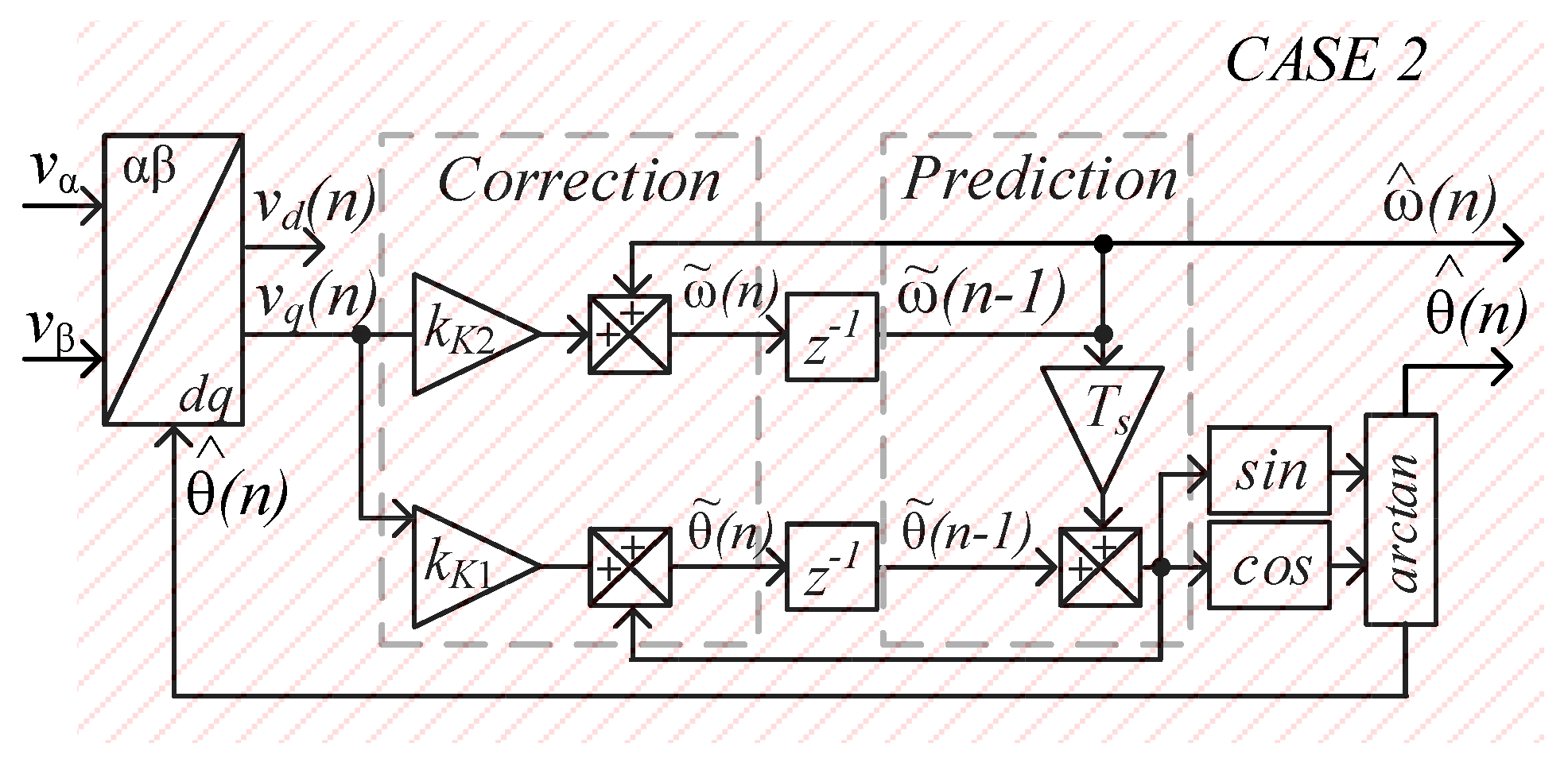
2.1. Kalman Filter Based Two-State Prediction Model

The implementation of the KFB two-state prediction model is proposed and evaluated in reference [29]. As shown in Figure 9, this block will operate on the comparison between prediction and correction states. The only difference from a genuine Kalman Filter is that the solution under study would have to adapt its gains for every processing time step, Ts. Its closed-loop transfer function, KFBTF, is given by Equation (13), where kK1 = k1/Ts = 2ζωn and kK2 = k2/Ts = ωn2. As in [29], ζ = 1/√2 and ωn = 125 rad/s are selected. The notations ^ and ~ represent estimated values as an output or intermediate signals of the system.
KFB TF ( s )   =   k K 2 s 2   +   sk K 1   +   k K 2

2.2. Modeling, Design Constraints and Procedure

This subsection will present the design procedure and modeling as a methodological model. The next section will include a design example, and Section 4 will present the experimental validation results. The first step is to define the limit frequencies for the desired operation range. These frequencies are the limit band frequencies, start and end (fls, fle). This is strictly a design choice. For example, for grid frequencies, the start and end can be set as 50 and 60 Hz, for AC motor applications they can be set as 10 and 100 Hz, and for HPA applications they can be set as 1 and 1000 Hz [9,10,11,12,13,14,15,16].
The second step is to determine the multiplier for achieving the correct bandwidth. The suggested gain (ς) is a decade further than the chosen bandwidth, but smaller or higher gains can be used to adjust the maximum phase added next to the start and end frequency limits (which will be detailed later). The resulting frequencies by the division, Equation (14), and multiplication, Equation (15), with ς are called the corner frequencies, initial and final (fci, fcf), respectively. Note that the corner frequencies match the IB pole moved from the origin, pi, and the DB placed pole, pd.
f ci   =   f ls ς
f cf   =   ς f le
Ideally, the same gain can be applied to both limits, but in the context where one wants to design an application in which there is a higher probability of using a specific frequency, a higher gain (ς1 and/or ς2) can be applied to that extreme, as shown in Equations (16) and (17). This will guarantee a gain close to the unitary and smaller phase for that specific frequency. The average gain can be found using (18), denoted by the ¯ symbol.
f ci   =   f ls ς 1
f cf   =   ς 2 f le
ς = ( ς 1   +   ς 2 ) 2
For both scenarios (same and different gains), a central cutoff frequency, fcc, must be found. This frequency will be equally distant by another gain, N, from fci and fcf on the logarithm distribution. The central frequency can be found as Equations (19) and (20). Compared to Figure 7, for pure integral and derivative functions, N would be equal to 0 rad/s because both functions have their 0 dB gain at 0 rad/s.
N   =   f cf f ci
f cc   =   N   f ci
The first part of the proposed topology can be built with analog amplifiers for analog implementations [40,41] or their corresponding transfer Equations (21) and (22) can be used as well in any digital-based application. The analog equivalent of the IBTF (21) is the integrator with controllable DC gain, shown in Figure 10, left. The DBTF (22) equivalent is the differentiator circuit with constant High Frequency (HF) gain, shown in Figure 9, right. The DC gain of the IBTF, when multiplied by the +20 dB/decade provided from the DBTF for those low frequencies, will cause the attenuation of frequencies outside the desired range of operation. Likewise, the HF gains of DBTF when multiplied for the −20 dB/decade from the IBTF will provide attenuation for frequencies higher than the desired range of frequencies.
IB TF ( s )   =   v i ( s ) v α ( s )   =   1 R i 1 C i 1 s   +   1 R i 2 C i   =   N 1 1   +   sR i 2 C i .
DB TF ( s )   =   v d ( s ) v α ( s )   =   R d 2 C d s sR d 1 C d   +   1   =   N 1 s   +   1 / ( R d 1 C d )
If implemented with the first part in analog mode, the gains of the integrators and differentiators for the whole operation range have to be carefully calculated to avoid saturation of the system, while considering the amplitude limits of the input. If implemented digitally using the related transfer functions, there is no risk of saturation. Even though using the transfer functions in digital applications is straightforward and easier with the constant improvements and developments on Rapid Control Prototyping, designing the system analogically can bring other benefits because it is pedagogical or approachable for some designers. Designing it in analog mode offers the designer the choice between the digital or analog implementation at the end, which is not the case when designed from the beginning in digital mode. In this study, the system is designed for analog but implemented in digital controllers (using their corresponding transfer functions) in order to evaluate the design and implementation procedures in both domains. The integrator with DC gain is a well-known element in electronics and its generic transfer function is shown in Figure 11a, with the gain on the top and the phase below. It provides controllable DC gain, Equation (23), for frequencies much smaller (denoted by the ≪) than the corner frequency, given by Equation (24), at the same location as the pole pi in Figure 7. A variable gain, ki/ω, for higher frequencies, is given by Equation (25). The cutoff frequency, where the absolute gain is unitary (0 dB), is defined as Equation (26) for the IB output.
IB TF (   f     f ci   )   =   N   =   R i 2 R i 1
f ci   =   1 2 π C i R i 2
IB TF (   f     f ci   )   =   1 R i 1 C i 1 2 π f
f cci   =   1 2 π C i R i 1
The transfer function of the differentiator with HF gain is shown in Figure 11b. It provides variable gain (kd/ω), as in Equation (27), with a slope of +20 dB/decade for frequencies much smaller (≪) than the corner frequency, Equation (28), at the same location as the pole pd in Figure 7. It also provides constant gain, Equation (29), for those frequencies higher than the corner, which is the same gain as kHF. The corner frequency should be higher than the end band frequency to ensure that the frequencies of the application are within the intended range. The cutoff frequency, where the gain is unitary (0 dB) is defined as Equation (30). The differential output has two important roles. The first one is to contribute with its differential part to the system, and to the multiplication that will follow. The second one is that the differential output has a phase of −90° with the input, and the function signal [vd] complements the square root of the squared cosine, as explained before.
DB TF (   f     f cf   )   =   R d 2 C d 2 π f
f cf   =   1 2 π C d R d 1
DB TF (   f     f cf   )   =   N   =   R d 2 R d 1
f ccd   =   1 2 π C d R d 2
By multiplying the integrator and differentiator gains, Equations (31) and (32), a unitary gain (0 dB) can be found for the desired frequency range (fls to fle), if the condition stated in Equation (33) is respected. In addition, there will be no phase (ideally) added to this signal, although a small phase error may be found close to the frequency limits. The corner frequencies are given by Equations (24) and Equation (28) and they must be equal, according to Equation (33). The unitary gain, as shown in any of the curves of Figure 12, in the entire range makes it possible to eliminate any further multiplication by gains, reducing the complexity of the proposed system.
IB TF DB TF ( s )   =   v i ( s ) v d ( s ) v α 2 ( s ) =   R i 2 R d 2 C d R i 1 1 1 + s ( R i 2 C i + R d 1 C d ) + s 2 ( R i 2 C i R d 1 C d )
| IB TF DB TF (   f ls   <   f   <   f le ) | =   R i 2 R d 2 C d R i 1 1 1   +   ( 2 π f ) ( R i 2 C i   +   R d 1 C d )   +   ( 2 π f ) 2 ( R i 2 C i R d 1 C d ) 1
f cc =   f ccd   =   1 2 π C d R d 2   =   f cci   =   1 2 π C i R i 1

3. Design Example

For the PA and PHIL application, the OSG must be able to recognize input frequencies from 1 to 1000 Hz. The initial gain (ς) used for the system is 10 and, as given by Equations (14) and (15), the corner frequencies will be 0.1 and 10,000 Hz. Using Equations (19) and (20), the gain Equation (34) and the central cutoff frequency Equation (35) will be expressed as
N   =   10000 / 0.1   =   316.227766
f cc   = f ccd   =   f cci   =   N   f ci   =   31.6277   Hz
Fixing the resistors Rd1 and Ri1 at 1 kΩ allows the remaining resistors Equation (36) to be found using Equations (23) and (29). Using Equations (26) and (30), it is possible to determine the capacitors for the integral and differential part, Equations (37) and (38). After having defined all the parameters, it is possible to determine the transfer functions for each block, Equations (21) and (22), and plot the amplitude and phase frequency response of the multiplication of both blocks, as shown in Figure 12, in the blue curve. The shadowed area represents the start and end frequency limits (1–1000 Hz). It is possible to observe the gain very close to unitary for all the operation range or AOI. There is a small phase error in the system next to limits (5.7° at 1 Hz and −5.7° at 1 kHz).
R i 2   = R d 2   = N   R i 1   =   316.2277   k Ω
C i   = 1 2 π f cci R i 1 =   5.0329   μ F
C d   = 1 2 π f ccd R d 2 =   15.915   nF
One solution to improve (and reduce the phase error next to the limit band frequencies) is to increase the gain (ς) to 20. The second case in Figure 12 is represented by the yellow line. Consequently, new values for N, resistors and capacitors are found in Equations (39)–(43). With a higher gain, there was an improvement on ensuring 0 dB (or unitary gain) in a more extended way. Most significantly, a phase error reduction on frequencies closer to the band limits was achieved through this process (2.86° at 1 Hz and −2.86° at 1 kHz).
N   =   632.4455
f cc   =   31.6277   Hz
R i 2   =   R d 2   =   N   R i 1   =   632.4555   k Ω
C i   =   5.0329   μ F
C d   =   7.9577   nF

4. Comparative Analysis of the Proposed System

In order to compare the proposed system APAF detection abilities, it will be benchmarked with another three topologies. The first one is the one from which the proposed topology is based, Picardi’s PLL [26], as shown in Figure 4. The gain C is set at 1/202, and the derivative pole is at 1.6 MHz, while the integral pole is at 0.5 Hz (although the study does not mention these poles they can be extracted from the passive elements used). The second system is the inverse Park’s PLL [31,32], as shown in Figure 3a. The filters are set with a cutoff of 120 Hz and kp = 200 and ki = 20,000. The third system is the Enhanced-PLL [33,34], with kp = 400 and ki = 40,000. The last two systems are set for a central frequency of 50 Hz.
All the results are simulated under the same time step of 10 μs (same as for experimental results in the next Section 5). The main aspect of the simulation is to evaluate the amplitude and frequency. Secondarily the error on the phase angle detection for all the systems will be evaluated. One important aspect of the simulations is that it is better to have smaller errors with higher settling times than the opposite, since high variations on APAF systems can create instability for converters or equipment dependent on them.
The first analysis is to evaluate the amplitude detection, Vm, for a wide range of frequencies, assessing the systems at 50 Hz, Figure 13a and 500 Hz, Figure 13b and zoom in Figure 13c. For 50 Hz, all the systems are able to detect the amplitude. At this condition, the best systems are the EPLL and Park’s PLL, since they are specifically designed for this frequency (both systems can be considered to have 0% error). The proposed system performs better than Picardi’s (0.2%), with 0.1% error. The error is related to the maximum overshoot or undershoot of the signal and all the averages perfectly match the 50 Hz input signal. For 500 Hz, the inability of Park’s PLL to track the amplitude is clear. EPLL was still able to track the amplitude correctly, with 0.1% error. Once again, the proposed system shows the superior performance when compared to Park’s PLL and Picardi’s, visible in Figure 13c. The proposed system outputted an error of 0.3%, smaller than the 0.8% from Picardi’s PLL. Except for EPLL’s, the proposed system showed remarkable results under this evaluation.
The second analysis takes into account the ability of the systems to identify the input signal’s frequency, for the same 50 and 500 Hz input and constant amplitude of 1 pu. As shown in Figure 14a, all systems are able to identify closely the input frequency of 50 Hz. Once again, for the fundamental frequency as same as the central frequency, Park’s PLL and EPLL performed at the best level, but once a different frequency was inputted, both systems lost their capacity of identifying the frequency, as can be seen in Figure 14b, for an input of 500 Hz. The proposed system was the best acting frequency detection for 500 Hz, with errors smaller than 0.44% (Picardi’s error is 0.7%). This shows the ability of the proposed system to deliver the frequency identification for a wide range of frequencies, without compromising the quality and precision of the output. As EPLL and Park’s PLL are designed for 50 Hz, they oscillate with high errors around that frequency.
The third analysis is very well known in the literature [29], that of evaluating the quality of APAF systems. This consists of applying a phase jump of 40° on the input signal, keeping the frequency and amplitude constant at 50 Hz and 1 pu. Several analyses can be done based on this, but the most important is the error of the phase angle (θ) when compared to the phase angle of the input signal, as shown in Figure 15. Picardi’s PLL and the proposed PLL are in phase, outputting the same result, since 50 Hz is inside both of their ranges of frequencies. The proposed system is the one with smaller overshoot/undershoot levels, reaching only 4.4° (measured at the highest oscillation after the 40° jump). Picardi’s PLL has a similar error of 4.57°. Parks’ PLL is the highest error overshoot (22.2°), followed by EPLL (11.19°).
Still under the 40° phase jump condition, the next analysis is on the ability of the systems to identify the input frequency. Figure 16a shows the results for an extended period, while Figure 16b focuses on the transient. EPPL suffers a high impulse, increasing the output frequency to 90.92 Hz (error of 81.84%). Park’s PLL undershoots a frequency of 36.61 Hz (error of 26.78%). Picardi’s PLL overshoots an output frequency 67.05 Hz (error of 34.1%). The proposed system on the other hand performs as the best frequency detection, with a small overshoot of 52.91 Hz (error of 5.82%), showing the remarkable stability of the system.
The last analysis for the same condition, the amplitude detection, Vm, will be evaluated. Figure 17a shows the extended period, while Figure 17b focuses on the initial part of the transient. The proposed PLL has a small overshoot (variation of 0.27 pu). Picardi’s PLL saturates its output (14.35 pu) even though that happens for a brief time. Park’s PLL gives the second highest ripple (variation of 0.4 pu), and EPLL for this condition does not present any overshoot, but mostly because the input matches its central frequency. The settling times for all systems are similar.
Now the systems can be evaluated at the last condition, which is a known effect in grids, the voltage sag. At a constant 50 Hz input, the amplitude changes from 1 pu to 0.7 pu. Shown in Figure 18a,b, the amplitude detection of all systems were evaluated. EPLL could not identify the signal variation, while Park’s PLL undershoots the highest error, with an output of 0.47 pu. The proposed system and Picardi’s present similar results, with an undershoot reaching 0.53 pu. Lastly, the frequency detection is evaluated in Figure 19a,b. Picardi’s PLL takes more than a second to settle and overshoots a signal of 63.4 Hz (error of 26.8%). EPLL is the worst undershoot, with 41.88 Hz (error 16.24%), but it has a short settling time. Park’s PLL is close to the last, with an undershoot of 42.55 Hz (error 14.9%). Once again, the proposed system shows the superior performance with a small error of 3.12%, with a small overshoot of 51.56 Hz.
All simulations show the ability of the proposed system to perform with high quality in all ranges of frequencies and amplitudes, differently from the other systems that can only perform well at one specific frequency. The proposed system even performs better for some conditions when comparing the other systems on their central frequency (50 Hz).

5. Experimental Validation of the System

Considering the good results achieved in the simulation, an experimental setup was built to validate the proposed system. The central element is the controller, an OPAL-RT OP4510 real-time simulator that will be used to process the input voltage and output its APAF and orthogonal signals. For its input and as a reference signal provider, a Hewlett Packard 3325B Synthesizer/Function Generator was used. A Yokogawa DLM2024 Mixed Signal Oscilloscope was used to read the input signal and the output signals of the controller. The controller was designed in Simulink environment. The minimum time step of 10 μs was used in this case. Table 1 presents the main parameters used for defining the variable of the system for the experimental tests. The experimental setup is presented in Figure 20.
Figure 21 shows the system that was built for validation, with the variables defined as Equations (39)–(43) and Table 1. The system includes the proposed OSG with unitary gain, a conventional amplitude detection and evaluates two cases for phase angle and frequency detection. In the first case, the limiters (LIM) were used to allow only positive values to be processed. The 2nd order Low Pass Filters (LPFs) were set to remove any high frequency noise or interferences from the amplitude and from the first case of frequency detection, with a cutoff of 100 Hz and 0.707 as damping factor.
Test (1) the verification of the system was performed initially with a frequency ramp to evaluate which one of the cases would perform a better frequency tracking. A ramp from 60 to 1000 Hz with a duration of 5 s (±188 Hz/s) was applied as the input signal, which also had amplitude steps around halfway of the ramp from 1 to 2, and later from 2 to 1 pu, as shown in Figure 22. The first graph shows in blue (CH1) the input voltage, the frequency reference in cyan (CH2), the frequency detection based on the derivative action (Case 1) in pink (CH3), and the frequency detection with Kalman Filters (Case 2) in green (CH4), which is overlapped with the reference. The middle graph shows the error between Case 1 and the reference (cyan—CH5), and between Case 2 and the reference (pink—CH6). The lower graph presents the zoomed areas detailing the amplitude steps. The results for Case 2 presented better quality, since the maximum error was a little higher than 5 Hz, while Case 1 was around 20 Hz. In addition, Case 1 presented a high transitory behavior when amplitude steps were applied. This case also showed an offset error that became more relevant in higher frequencies. As the quality of Case 2 is superior, it is clear that the system with Kalman Filter will be selected as a standard for frequency identification for the next tests.
Test (2) comprehends an amplitude step given to the reference (blue—CH1) from 1 to 2 pu and later removed. As shown in Figure 23. The amplitude detection’ signal output, Vm, appears in the cyan line (CH2). The reference frequency and the Case 2 detection output are also shown (pink-CH3 and green-CH4). The lower graph shows the zoomed areas 1 and 2. The amplitude detection system could track the new signal parameters within two and a half cycles of the new signal, showing the quality of the proposed system in tracking wide variations in amplitude.
Test (3) realizes a frequency step given to the reference (blue—CH1) from 500 to 750 Hz, and later removed, Figure 24. The amplitude detection’ signal output, Vm, is shown in the cyan line (CH2), similar to the previous test. The reference frequency (pink—CH3) and the frequency detection output of Case 2 are shown in the pink and green lines (CH3 and CH4, respectively). Different from the amplitude, the frequency detection takes a few more cycles to achieve steady state, around 25 cycles (35 ms) for the increasing step and 15 (20 ms) for the decreasing. Even though it is a considerable high step (±50%), the detection was fast when only analyzing the point of view of time. The processor time step plays a major role in limiting this speed of response. There is no significant or observable impact of the frequency step on the amplitude detection, which exhibits the superior quality of the combination of the proposed system with the Kalman’s Filter Based frequency detection.
Test (4), the phase angle detection, together with the amplitude detection are the most important signal’s parameters for the applications under study. Therefore, lastly and most importantly, this test will evaluate the ability of the system to generate appropriate orthogonal signals (pink—CH3) and the phase angle (green—CH4) of the input signal (blue—CH1), as shown in Figure 25. In addition, the amplitude detection is presented (cyan—CH2). A phase inversion is applied and detailed on the zoomed area below. For this set of results, the speed of response of the system adapts remarkably to the variation on the input signal, without creating any overshoot in Vm and instantaneously detecting and correcting the phase angle output.
When looking back at the theorems and challenges proposed at the end of Section 1, it is safe to say that (i) was achieved with an intuitive design, simulation and validation for a system capable of identifying wide ranges of frequency and amplitude; (ii) was achieved by presenting a unitary C (Picardi’s PPL C) gain that can be eliminated on the proposed system, making it simpler and less tend to errors; (iii) was achieved in Section 4, with solid results in comparison with available techniques; (iv) was achieved in detail in Section 3; (v) was introduced in Section 2 (Section 2.1), used on simulations in Section 4 and validated experimentally as the best solution for frequency identification with vα and vβ as inputs; (vi) was detailed in this section.
Considering the simulations, the proposed system was the best performing APAF in several cases and the only one able to perform with small errors at all ranges of the input signal. This performance was validated experimentally in this section, proving this topology ability to identify single-phase inputs for diverse application.

6. Conclusions

The main benefit of the topology built is the ability to identify a single-phase signal with a wide range of frequency and amplitude, while the majority of studies operates only at a given and known frequency. The dynamic of the proposed system achieved a very fast response for the orthogonal signal generation, amplitude and phase angle detection. For frequency detection, two techniques were evaluated and the second case, a Kalman Filter Based solution provided better results for steady state and transient conditions. In addition, the proposed design procedure, which was built in a more straightforward way, enables the system to be either implemented with analog or digital devices. A set of experimental tests were performed to validate the study, under a wide range of frequency and amplitudes.
For future studies, the integration of the proposed APAF with actual equipment, such as grid-tied converters or Hybrid Power Amplifiers can be mentioned. In addition, the performance of the proposed solution in combination with another equipment can be again benchmarked against known APAF techniques. The system can also be improved to perform under common grid anomalies not covered in the scope of this work, such as the presence of low order harmonics, noise, DC level or more severe step variations in amplitude, frequency and/or phase angle.

Author Contributions

Conceptualization, L.M.K.; data curation, L.M.K.; formal analysis, L.M.K. and L.A.C.L.; funding acquisition, L.A.C.L.; investigation, L.M.K.; methodology, L.M.K.; project administration, L.A.C.L.; resources, L.A.C.L.; software, L.M.K.; supervision, L.A.C.L.; validation, L.M.K. and L.A.C.L.; visualization, L.M.K.; writing—original draft, L.M.K.; writing—review and editing, L.A.C.L. All authors have read and agreed to the published version of the manuscript.

Funding

This work is founded by the National Sciences & Engineering Research Council of Canada and Concordia University as part of InnovÉÉ/NSERC CRD project.

Acknowledgments

The authors thank OPAL-RT for all the support during the development of this project.

Conflicts of Interest

The authors declare no conflict of interest.

References

  1. Blaabjerg, F.; Teodorescu, R.; Liserre, M.; Timbus, A. Overview of Control and Grid Synchronization for Distributed Power Generation Systems. IEEE Trans. Ind. Electron. 2006, 53, 1398–1409. [Google Scholar] [CrossRef] [Green Version]
  2. Han, Y.; Luo, M.; Zhao, X.; Guerrero, J.M.; Xu, L.; Han, Y.; Luo, M.; Zhao, X.; Guerrero, J.M.; Xu, L. Comparative Performance Evaluation of Orthogonal-Signal-Generators-Based Single-Phase PLL Algorithms–A Survey. IEEE Trans. Power Electron. 2015, 31, 3932–3944. [Google Scholar] [CrossRef] [Green Version]
  3. Golestan, S.; Monfared, M.; Freijedo, F.D.; Guerrero, J.M. Dynamics Assessment of Advanced Single-Phase PLL Structures. IEEE Trans. Ind. Electron. 2012, 60, 2167–2177. [Google Scholar] [CrossRef]
  4. Shitole, A.B.; Suryawanshi, H.M.; Sathyan, S. Comparative evaluation of synchronization techniques for grid interconnection of renewable energy sources. In Proceedings of the IECON 2015-41st Annual Conference of the IEEE Industrial Electronics Society, Yokohama, Japan, 9–12 November 2015; pp. 1436–1441. [Google Scholar]
  5. Xiao, F.; Dong, L.; Li, L.; Liao, X. Fast voltage detection method for grid-tied renewable energy generation systems under distorted grid voltage conditions. IET Power Electron. 2017, 10, 1487–1493. [Google Scholar] [CrossRef]
  6. Guo, C.; Liu, W.; Zhao, C.; Iravani, R. A Frequency-Based Synchronization Approach for the VSC-HVDC Station Connected to a Weak AC Grid. IEEE Trans. Power Deliv. 2017, 32, 1460–1470. [Google Scholar] [CrossRef]
  7. Carrasco, J.; Franquelo, L.G.; Bialasiewicz, J.; Galvan, E.; Portillo, R.; Prats, M.; Leon, J.I.; Moreno, N. Power-Electronic Systems for the Grid Integration of Renewable Energy Sources: A Survey. IEEE Trans. Ind. Electron. 2006, 53, 1002–1016. [Google Scholar] [CrossRef]
  8. Golestan, S.; Monfared, M.; Freijedo, F.D.; Guerrero, J.M. Design and Tuning of a Modified Power-Based PLL for Single-Phase Grid-Connected Power Conditioning Systems. IEEE Trans. Power Electron. 2012, 27, 3639–3650. [Google Scholar] [CrossRef] [Green Version]
  9. Maniatopoulos, M.; Lagos, D.; Kotsampopoulos, P.; Hatziargyriou, N. Combined control and power hardware in-the-loop simulation for testing smart grid control algorithms. IET Gener. Transm. Distrib. 2017, 11, 3009–3018. [Google Scholar] [CrossRef]
  10. Kunzler, L.M.; Lopes, L.A.C. Power balance technique for cascaded H-bridge multilevel cells in a hybrid power amplifier with wide output voltage range. In Proceedings of the 2018 IEEE International Conference on Industrial Technology (ICIT), Lyon, France, 20–22 February 2018; pp. 800–805. [Google Scholar]
  11. Kunzler, L.M.; Lopes, L.A.C. Hybrid Single Phase Wide Range Amplitude and Frequency Detection with Fast Reference Tracking. In Proceedings of the 2019 IEEE 28th International Symposium on Industrial Electronics (ISIE), Vancouver, BC, Canada, 12–14 June 2019; pp. 878–883. [Google Scholar] [CrossRef]
  12. Kunzler, L.M.; Lopes, L.A.C. Algorithm for Improving Power Balance for Cascaded H-Bridge Multilevel under Staircase Modulation for Linear Loads. In Proceedings of the IECON 2019-45th Annual Conference of the IEEE Industrial Electronics Society, Lisbon, Portugal, 14–17 October 2019; Volume 1, pp. 6066–6071. [Google Scholar]
  13. Singh, B.P.; Arya, S.R. Implementation of Single-Phase Enhanced Phase-Locked Loop-Based Control Algorithm for Three-Phase DSTATCOM. IEEE Trans. Power Deliv. 2013, 28, 1516–1524. [Google Scholar] [CrossRef]
  14. Zhang, Q.; Sun, X.-D.; Zhong, Y.; Matsui, M.; Ren, B.-Y. Analysis and Design of a Digital Phase-Locked Loop for Single-Phase Grid-Connected Power Conversion Systems. IEEE Trans. Ind. Electron. 2010, 58, 3581–3592. [Google Scholar] [CrossRef]
  15. Masadeh, M.A.; Amitkumar, K.S.; Pillay, P. Power Electronic Converter-Based Induction Motor Emulator Including Main and Leakage Flux Saturation. IEEE Trans. Transp. Electrif. 2018, 4, 483–493. [Google Scholar] [CrossRef]
  16. Amitkumar, K.S.; Thike, R.; Pillay, P. Linear Amplifier-Based Power-Hardware-in-the-Loop Emulation of a Variable Flux Machine. IEEE Trans. Ind. Appl. 2019, 55, 4624–4632. [Google Scholar] [CrossRef]
  17. IEEE Standard for Interconnection and Interoperability of Distributed Energy Resources with Associated Electric Power Systems Interfaces; IEEE-SASB Coordinating Committees: Piscataway, NJ, USA, 2018. [CrossRef]
  18. Cossutta, P.; Raffo, S.; Cao, A.; DiTaranto, F.; Aguirre, M.P.; Valla, M.I. High speed single phase SOGI-PLL with high resolution implementation on an FPGA. In Proceedings of the 2015 IEEE 24th International Symposium on Industrial Electronics (ISIE), Janeiro, Brazil, 3–5 June 2015; pp. 1004–1009. [Google Scholar]
  19. Ciobotaru, M.; Teodorescu, R.; Blaabjerg, F. A New Single-Phase PLL Structure Based on Second Order Generalized Integrator. In Proceedings of the 37th IEEE Power Electronics Specialists Conference, Jeju, Korea, 18–22 June 2006. [Google Scholar]
  20. Golestan, S.; Guerrero, J.M.; Vidal, A.; Yepes, A.G.; Doval-Gandoy, J.; Freijedo, F.D.; Golestam, S.; Guerrero, J.M.; Vidal, A.; Yepes, A.G.; et al. Small-Signal Modeling, Stability Analysis and Design Optimization of Single-Phase Delay-Based PLLs. IEEE Trans. Power Electron. 2015, 31, 3517–3527. [Google Scholar] [CrossRef] [Green Version]
  21. Hou, M. Estimation of Sinusoidal Frequencies and Amplitudes Using Adaptive Identifier and Observer. IEEE Trans. Autom. Control. 2007, 52, 493–499. [Google Scholar] [CrossRef]
  22. Yazdani, D.; Bakhshai, A.; Joos, G.; Mojiri, M. A nonlinear adaptive synchronization technique for single-phase grid-connected converters. In Proceedings of the 2008 IEEE Power Electronics Specialists Conference, Rhodes, Greece, 15–19 June 2008; pp. 4076–4079. [Google Scholar]
  23. Yin, G.; Guo, L.; Li, X. An Amplitude Adaptive Notch Filter for Grid Signal Processing. IEEE Trans. Power Electron. 2012, 28, 2638–2641. [Google Scholar] [CrossRef]
  24. Robles, E.; Ceballos, S.; Pou, J.; Martín, J.L.; Zaragoza, J.; Ibañez, P. Variable-Frequency Grid-Sequence Detector Based on a Quasi-Ideal Low-Pass Filter Stage and a Phase-Locked Loop. IEEE Trans. Power Electron. 2010, 25, 2552–2563. [Google Scholar] [CrossRef] [Green Version]
  25. Robles, E.; Pou, J.; Ceballos, S.; Zaragoza, J.; Martín, J.L.; Ibañez, P. Frequency-Adaptive Stationary-Reference-Frame Grid Voltage Sequence Detector for Distributed Generation Systems. IEEE Trans. Ind. Electron. 2010, 58, 4275–4287. [Google Scholar] [CrossRef]
  26. Picardi, C.; Sgro, D.; Gioffre, G. A simple and low-cost PLL structure for single-phase grid-connected inverters. SPEEDAM 2010 2010, 358–362. [Google Scholar] [CrossRef]
  27. Burger, B.; Engler, A. Fast signal conditioning in single phase systems. In Proceedings of the 9th European Conference on Power Electronics and Applications, Graz, Austria, 27–29 August 2001. [Google Scholar]
  28. Ozdemir, A.; Vural, C.; Yazici, I. Fast and robust software-based digital phase-locked loop for power electronics applications. IET Gener. Transm. Distrib. 2013, 7, 1435–1441. [Google Scholar] [CrossRef]
  29. Golestan, S.; Guerrero, J.M.; Vasquez, J.C. Steady-State Linear Kalman Filter-Based PLLs for Power Applications: A Second Look. IEEE Trans. Ind. Electron. 2018, 65, 9795–9800. [Google Scholar] [CrossRef] [Green Version]
  30. Vila-Valls, J.; Closas, P.; Navarro, M.; Fernández-Prades, C. Are PLLs dead? A tutorial on kalman filter-based techniques for digital carrier synchronization. IEEE Aerosp. Electron. Syst. Mag. 2017, 32, 28–45. [Google Scholar] [CrossRef]
  31. Silva, S.; Lopes, B.; Filho, B.C.; Campana, R.; Boaventura, W. Performance evaluation of PLL algorithms for single-phase grid-connected systems. In Proceedings of the 39th IAS Annual Meeting, Seattle, WA, USA, 3–7 October 2004. [Google Scholar] [CrossRef]
  32. Arruda, L.N.; Silva, S.M.; Filho, B.J.C. PLL structures for utility connected systems. In Proceedings of the Conference Record of the 2001 IEEE Industry Applications Conference 36th IAS Annual Meeting (Cat No 01CH37248) IAS-01, Chicago, IL, USA, 30 September–4 October 2001. [Google Scholar] [CrossRef]
  33. Karimi-Ghartemani, M.; Iravani, M. A Method for Synchronization of Power Electronic Converters in Polluted and Variable-Frequency Environments. IEEE Trans. Power Syst. 2004, 19, 1263–1270. [Google Scholar] [CrossRef]
  34. Karimi-Ghartemani, M.; Iravani, M. A new phase-locked loop (PLL) system. In Proceedings of the 44th IEEE 2001 Midwest Symposium on Circuits and Systems. MWSCAS 2001 (Cat. No.01CH37257), Dayton, OH, USA, 14–17 August 2001; Volume 1, pp. 421–424. [Google Scholar] [CrossRef]
  35. Reza, S.; Ciobotaru, M.; Agelidis, V. Robust technique for accurate estimation of single-phase grid voltage fundamental frequency and amplitude. IET Gener. Transm. Distrib. 2015, 9, 183–192. [Google Scholar] [CrossRef]
  36. Xiong, L.; Zhuo, F.; Wang, F.; Liu, X.; Zhu, M. A Fast Orthogonal Signal-Generation Algorithm Characterized by Noise Immunity and High Accuracy for Single-Phase Grid. IEEE Trans. Power Electron. 2015, 31, 1847–1851. [Google Scholar] [CrossRef]
  37. Ikken, N.; Bouknadel, A.; Haddou, A.; Tariba, N.-E.; El Omari, H.; El Omari, H. PLL Synchronization Method Based on Second-Order Generalized Integrator for Single Phase Grid Connected Inverters Systems during Grid Abnormalities. In Proceedings of the 2019 International Conference on Wireless Technologies, Embedded and Intelligent Systems (WITS), Fez, Morocco, 3–5 April 2019; pp. 1–5. [Google Scholar] [CrossRef]
  38. Bei, T.-Z.; Wang, P. Robust frequency-locked loop algorithm for grid synchronisation of single-phase applications under distorted grid conditions. IET Gener. Transm. Distrib. 2016, 10, 2593–2600. [Google Scholar] [CrossRef]
  39. Shah, S.; Parsa, L. Small-signal modeling of single-phase PLLs using harmonic signal-flow graphs. In Proceedings of the 2017 IEEE Energy Conversion Congress and Exposition (ECCE), Cincinnati, OH, USA, 1–5 October 2017; pp. 4989–4995. [Google Scholar] [CrossRef]
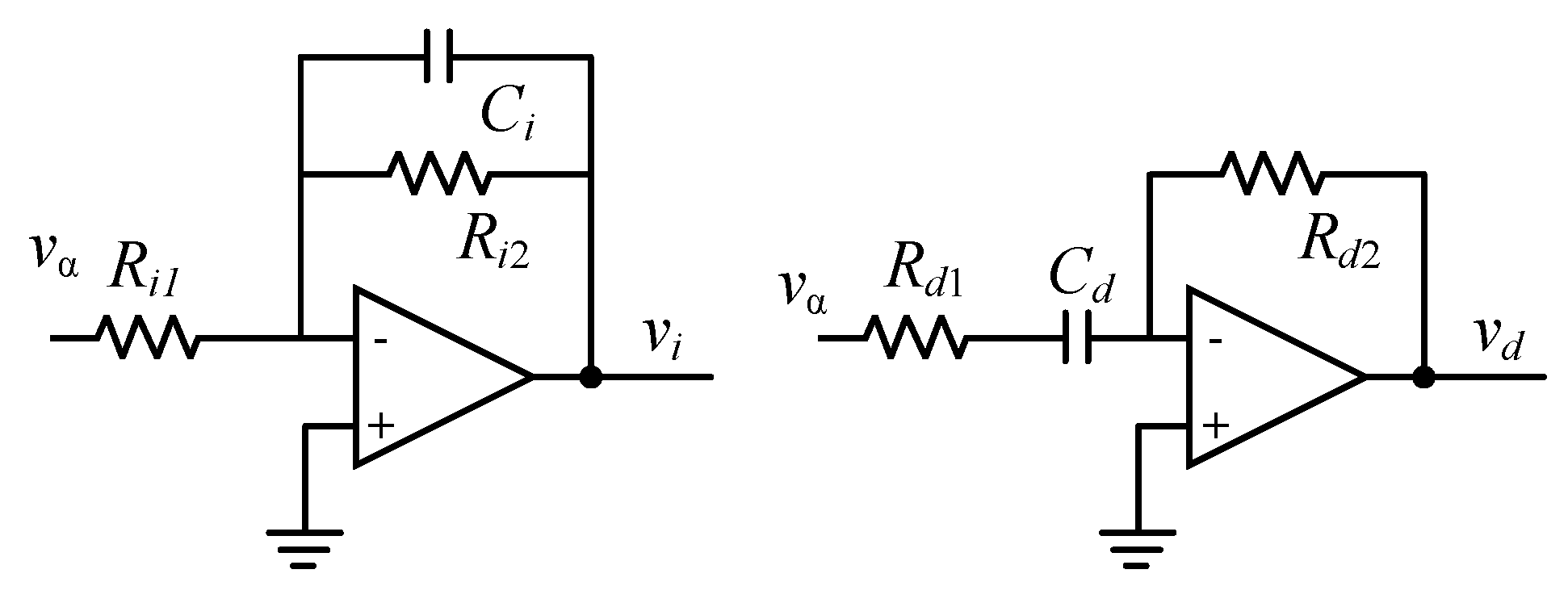
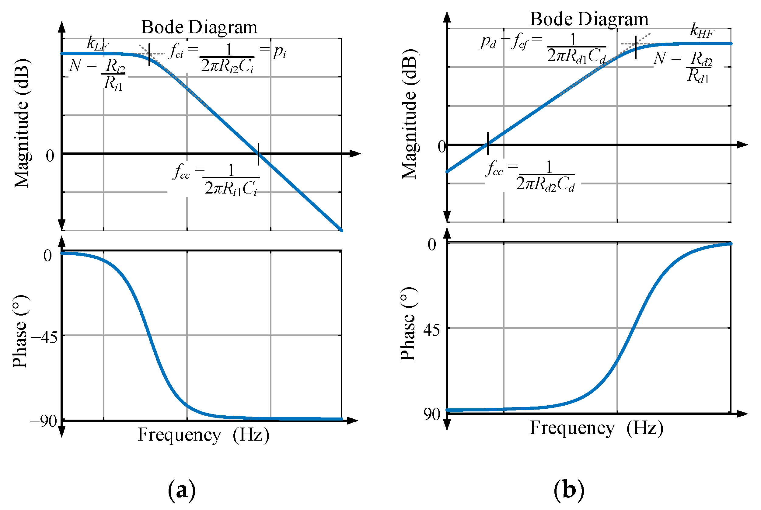
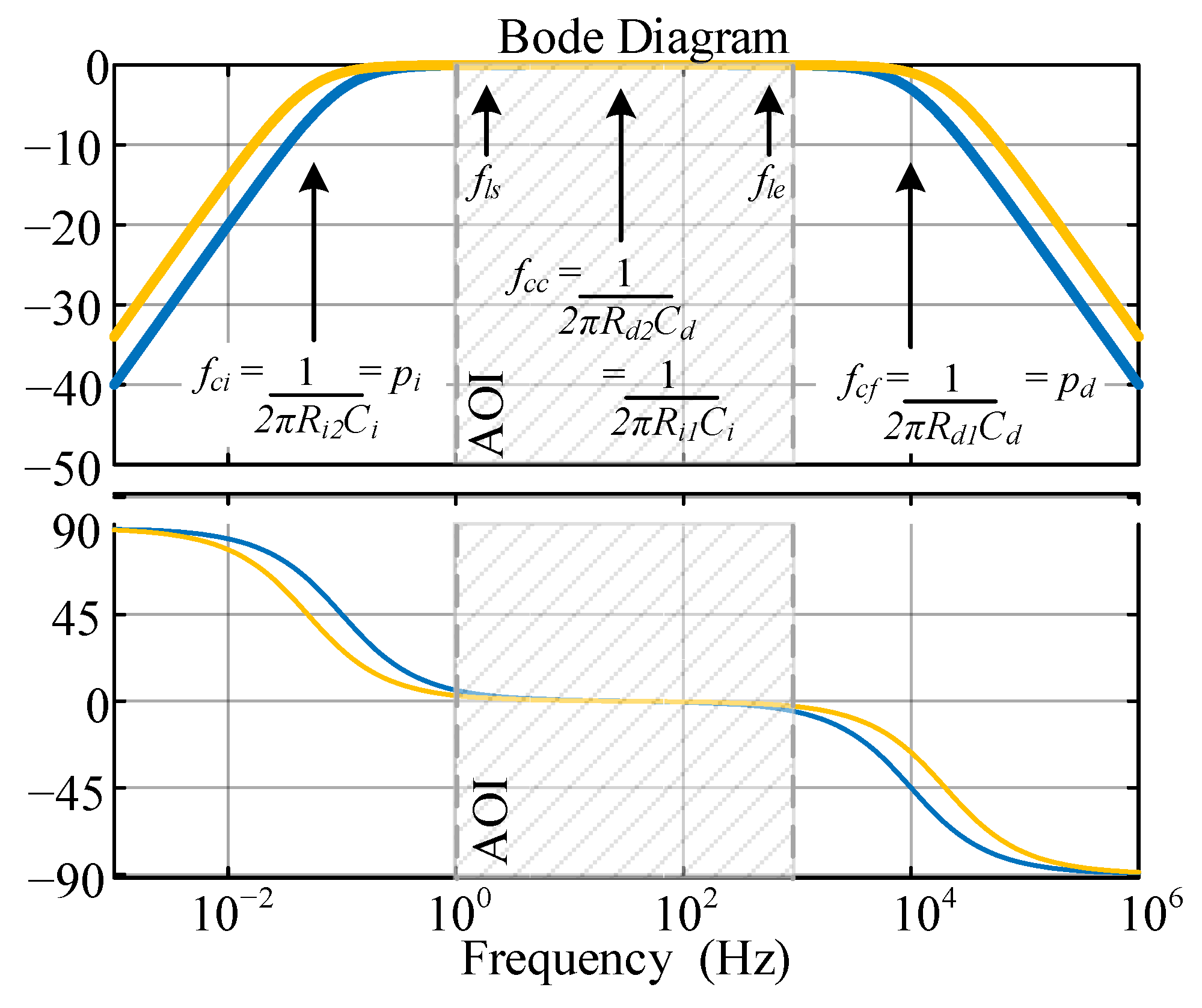
  40. Integrator Circuit. Analog Engineer’s Circuit: Amplifiers (Application Report No. SBOA275A), February 2018 (revised January 2019). Available online: http://www.ti.com/lit/an/sboa275a/sboa275a.pdf (accessed on 24 August 2020).
  41. Differentiator Circuit. Analog Engineer’s Circuit: Amplifiers (Application Report No. SBOA276A), February 2018 (revised January 2019). Available online: http://www.ti.com/lit/an/sboa275a/sboa276a.pdf (accessed on 24 August 2020).
Figure 1. Conventional single-phase Phase-Locked Loop (PLL) with Orthogonal Signal Generation.
Electronics 09 01578 g001
Figure 2. Second Order Generalized Integrator as Orthogonal Signal Generation (OSG).
Electronics 09 01578 g002
Figure 3. (a) Inverse Park’s PLL; (b) enhanced-PLL.
Electronics 09 01578 g003
Figure 4. Derivative-Integral frequency independent OSG [26].
Electronics 09 01578 g004
Figure 5. Steps to build the IBTF from a pure integral function (blue—no gains | red—with gains | pink—with gains and added/displaced poles).
Electronics 09 01578 g005
Figure 6. Steps to build the DB transfer function (DBTF) from a pure derivative function (blue—no gains | red—with gains | pink—with gains and added/displaced poles).
Electronics 09 01578 g006
Figure 7. Results from the multiplication of pure and modified integral and derivative functions (blue—no gains | red—with gains | pink—with gains and added/displaced poles).
Electronics 09 01578 g007
Figure 8. Proposed wide band frequency detection system.
Electronics 09 01578 g008
Figure 9. Second case for the frequency detection based on the orthogonal signals input and a Kalman Filter Based solution.
Electronics 09 01578 g009
Figure 10. Integrator and differentiator for analog implementation.
Electronics 09 01578 g010
Figure 11. Frequency response with gain (top) and phase (below) (a) integral block; (b) derivative block.
Electronics 09 01578 g011
Figure 12. Result of the multiplication of vd and vi for design example—amplitude (top) phase (below)—first case (ς = 10) in blue, second in orange (ς = 20).
Electronics 09 01578 g012
Figure 13. Comparison of amplitude detection techniques for a 1 pu input of (a) 50 Hz; (b) 500 Hz; (c) zoomed 500 Hz.
Electronics 09 01578 g013
Figure 14. Comparison of frequency detection techniques for a 1 pu input of (a) 50 Hz; (b) 500 Hz.
Electronics 09 01578 g014
Figure 15. Comparison of phase angle detection errors for a 40° phase jump for a 1 pu and 50 Hz input.
Electronics 09 01578 g015
Figure 16. Comparison of frequency detection techniques for a 40° phase jump for a 1 pu (a) 50 Hz; (b) zoomed for 50 Hz.
Electronics 09 01578 g016
Figure 17. Comparison of amplitude detection techniques for a 40° phase jump for a 1 pu (50 Hz) input for (a) extended frame; (b) zoomed frame (same legend).
Electronics 09 01578 g017
Figure 18. Comparison of amplitude detection techniques for a voltage sag from 1 to 0.7 pu (50 Hz) for (a) extended frame; (b) zoomed frame.
Electronics 09 01578 g018
Figure 19. Comparison of frequency detection techniques for a voltage sag from 1 to 0.7 pu (50 Hz) for (a) extended frame; (b) zoomed frame (same legend).
Electronics 09 01578 g019
Figure 20. Experimental setup built for the system validation.
Electronics 09 01578 g020
Figure 21. Complete system used for the validation of the proposed OSG and frequency/amplitude detection system.
Electronics 09 01578 g021
Figure 22. Experimental results related do Test 1—frequency ramp (±188 Hz/s) and voltages steps 1-2-1 pu.
Electronics 09 01578 g022
Figure 23. Experimental results related do Test 2—amplitude steps 1-2-1 pu.
Electronics 09 01578 g023
Figure 24. Experimental results related do Test 3—frequency steps 500-750-500 Hz.
Electronics 09 01578 g024
Figure 25. Experimental results related do Test 4—orthogonal signal generation and phase angle for a phase inversion.
Electronics 09 01578 g025
Table 1. Parameters for experimental setup.
ParameterValue OR Range
Input signal amplitude (vα)0.5–2 pu
Input signal frequency (vα)1–1000 Hz
Rd1 & Ri11 kΩ
Rd2 & Ri2632.4555 kΩ
Cd7.9577 nF
Ci5.0329 μF
ki−0.005032
kd−198.692602
kK10.01768 [29]
kK21.5625 [29]
Processor time step (Ts)10 µs

