Blockage Detection in Pipeline Based on the Extended Kalman Filter Observer

Abstract

Currently numerous approaches with various applicability have been generated in order to detect damage in pipe networks. Pipeline faults such as leaks and partial or complete blockages usually create serious problems for engineers. The model-based leak, as well as block detection methods for the pipeline systems gets more and more attention. Among these model-based methods, the state observer and state feedback based methods are usually used. While the observability, as well as controllability, are taken to be the prerequisites for utilizing these techniques. In this work, a new technique based on the extended Kalman filter observer is proposed in order to detect and locate the blockage in the pipeline. Furthermore, the analysis of observability and controllability in the pipe networks is investigated. Important theorems are given for testing the observability as well as controllability of the pipeline system.

1. Introduction

Leaks, as well as partial or complete blockages, can be considered as a usual fault arising in pipelines that creates troubles [1,2,3,4]. Leaks result in loss of fluid that causes a loss in pressure, efficiency as well as economic expense, also on occasions it may impact the environment. Blockage barricade flow, which causes a loss in pressure, and so enhances the required pumping expenses in order to dominate the loss in pressure, also occasionally blockage results in absolute termination of functioning [5,6]. Advanced diagnosis, as well as an exact place of leaks or blockages, can help in avoiding the troubles created by such faults and also develop the correct timing decision in order to deal with faults for preventing or diminishing production/performance suspension [7,8,9,10,11].

Blockages have been classified based on their physical extent related to the entire length of the system. Localized contractions, which are taken to be point discontinuities, are defined as discrete blockages. Blockages that contain remarkable length related to the entire pipe length are defined as extended blockages [12]. Dissimilar to the leaks inside piping systems, blockages do not produce obvious exterior indicators for their location to be mentioned as the release and agglomeration of fluids surrounding the pipe. Oftentimes intrusive approaches, utilizing devices the insertion of a closed-circuit camera or a robotic PIG (pipeline intervention gadget), are needed in order to specify the place of blockages. Insertion of a camera or robotic pig can lead to several uncertainties related to the speed of travel and the distance of travel in the midst of the insertion point and the blockage such that on many occasions cases the camera or the robotic pig is trapped into the blockage and leads to greater trouble in this case compared with the appearance of the blockage solely.

Recently, flow analysis is developed on the basis of efficient methods in order to identify blockages. The developed techniques utilize fluid transients according to the responding of the system to an injected transient in order to detect, locate, as well as to measure blockages, which have demonstrated a promising development. In [13,14] a time reflection technique is suggested in order to detect partial blockage of discrete and extended types in a single pipeline for different numbers of blockages. In [15] an impulse response technique is proposed in order to detect leaks as well as partial blockages of discrete type in a single pipeline, and also the technique is tested numerically. In [16] the authors used the damping of fluid transients on the basis of the analytical solution as well as experimental verifications in order to detect partial single discrete blockage in a single pipeline. In [17] the numerical outcomes with laboratory experiments are compared and concluded that the blockage location can be identified with nearly no error, whilst the size identification contains some errors.

The recent published research findings are more dependent on designing the observer, controller or fault identification approaches [18,19,20,21,22,23,24]. In this work, a novel method is proposed in order to analyse pipeline system, generally for identification and location of blockage using model-based techniques and extended Kalman filter observer. The modelling process is based on discretization with the finite-difference technique of classical mass as well as continuity equations. The discretization results in a system of ordinary differential equations with boundary conditions, which demonstrate faults as well as pipeline accessories. The states of the produced system are flows, pressure heads, the blockage and a parameter concerned with the blockage intensity. In continuous-time, a nonlinear system is used for designing observers. Observers are commonly on the basis of a conversion of the treated system into a triangular observable form accordingly, the variables that are straightly estimated correlate with the output derivatives. Furthermore, in this paper, the observability and the controllability of the pipe networks are investigated.

2. Pipeline Modelling

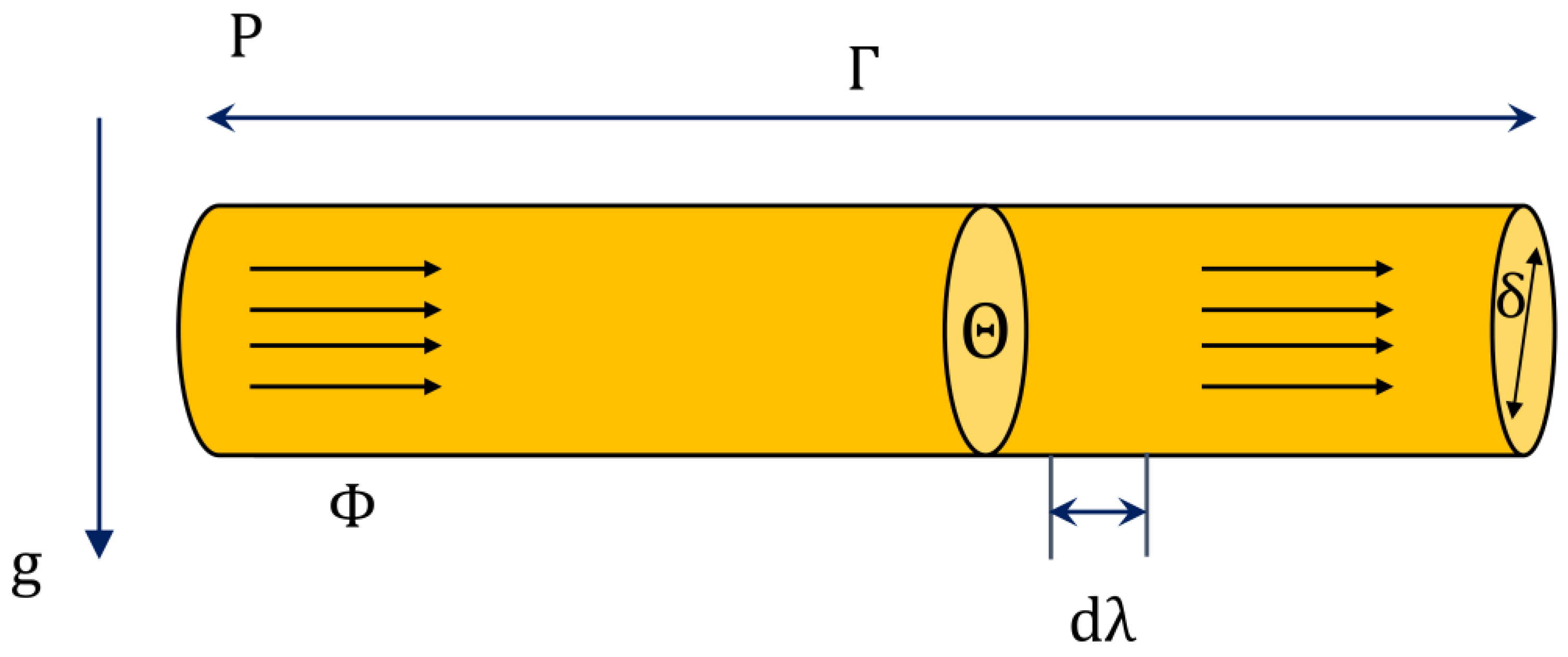
Here, we neglected the convective variation in velocity, also the compressibility in the line of length $(\Gamma )$. The liquid density ($\rho$), the flow rate $(\Phi )$ and also pressure $\left(\mathsf{{\rm P}}\right)$ at the entry and exit of the pipe can be measured for evaluation. The cross-sectional region $(\Theta )$ related to the pipe was taken to be fixed all over the pipe system. The feature of the pipe is illustrated in Figure 1.

For acquiring the mass and momentum in hydrodynamics utilizing Newton’s second law ($F=ma$) to a control volume in the continuum and body force pipe [25] (ρ $=\frac{f}{2\delta }v$) the below-mentioned equation can be developed,

$$\frac{\partial v}{\partial t}+\frac{1}{\rho }\frac{\partial p}{\partial \lambda }+\frac{f}{2\delta }v=0.$$

(1)

By substituting $v=\frac{\Phi }{\Theta }$ and $p=\rho g\Pi$ in (1) the following relation is gotten,

$$\frac{\partial (\frac{\Phi }{\Theta })}{\partial t}+\frac{1}{\rho }\frac{\partial (\rho g\Pi )}{\partial \lambda }+\frac{f}{2\delta }(\frac{\Phi }{\Theta })=0,$$

(2)

which may be simplified as

$$\frac{\partial (\Phi )}{\Theta \partial t}+\frac{\rho g}{\rho }\frac{\partial (\Pi )}{\partial \lambda }+\frac{f}{2\delta \Theta }\Phi =0.$$

(3)

This equation may be written as

$$\frac{\partial \Phi }{\partial t}+\Theta g\frac{\partial }{\partial \lambda }H+\frac{f\Phi }{2\delta }=0,$$

(4)

where $\Pi$ is taken to be the pressure head $\left(m\right)$, $\Phi$ is taken to be the flow rate ($m^3/s$), $\lambda$ is considered as the length coordinate $\left(m\right)$, $t$ is considered as the time coordinate $\left(s\right)$, $g$ is taken to be the gravity $\left(m/s^2\right)$, $\Theta$ is taken to be the section area $\left(m^2\right)$, $\delta$ is taken to be the diameter $\left(m\right)$ and $f$ is considered as the friction coefficient.

In most work the friction coefficient is fixed, even if it is sometimes updated known to depend on the so-called Reynolds number $\left(Re\right)$ and the roughness friction coefficient of the pipe $\left(e\right)$. The Swamee–Jain equation [26] describes this friction coefficient value for a pipe with a circular section of diameter $\left(\delta \right)$ as:

$$f={\left(\frac{0.5}{\ln [0.27\left(\frac{e}{\delta }\right)+5.74\frac{1}{R{e}^{0.9}}]}\right)}^2.$$

(5)

Such that,

$$Re=4\frac{\rho \Phi }{\pi \delta \mu }=\frac{\rho v\delta }{\mu },$$

(6)

where $\rho$ is the fluid density and $\mu$ is the fluid viscosity. Equation (5) is valid for ${10}^{-8}<\frac{e}{\delta }<0.01$ and $5000<Re<{10}^8$.

The continuity equation can be defined as follows for the pipeline system,

$$\frac{\partial p}{\partial t}+\rho a^2\frac{\partial v}{\partial \lambda }=0.$$

(7)

Replacing the pressure head $(\Pi )$ as well as the flow rate $(\Phi )$ in Equation (7), we have,

$$\frac{\partial \Pi }{\partial t}+\frac{a^2}{g\Theta }\frac{\partial \Phi }{\partial \lambda }=0.$$

(8)

Such that $a$ is taken to be the velocity of the pressure wave $\left(m/s\right)$.

The pressure head $(\Pi )$ and flow rate $(\Phi )$ are taken to be functions of position and time as $\Pi \left(x,t\right)$ and $\Phi \left(x,t\right)$, such that $\lambda \in \left[0,\Gamma \right]$, where $\Gamma$ is the pipe length.

If a system has minor variations we have,

$$\frac{\partial \Phi }{\partial t}+\Theta g\frac{\partial }{\partial \lambda }\Pi +\frac{f\Phi }{\delta \Theta }=0.$$

(9)

3. Blockage Modelling

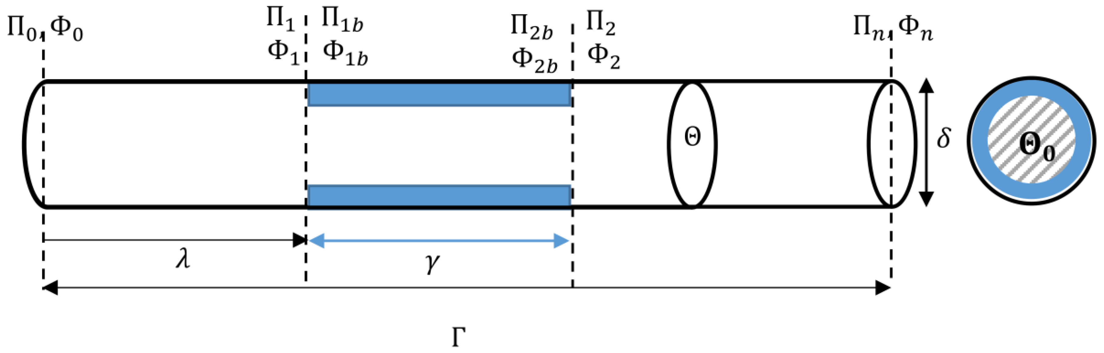
Blockages have been considered as usual faults in pipes as well as pipeline networks. They can be generated because of the agglomeration of the transported fluid or the partial block of a valve. A blocked is a reduced cross-sectional area of the pipe with significant length $\gamma$. For modelling the blocked stretch (see Figure 2), the blockage region, displayed by ${\Theta }_b$, is expressed as a percentage of the pipe region $\Theta$. The subscript $b$ signifies the blockage.

Pressure $H_1$ varies due to the blockage and this changed pressure is displayed by $H_{1b}$.

A mathematical expression for a blockage can be deduced from the Bernoulli’s equation, which relates the pressure difference between the pipeline inside and outside. Bernoulli’s equation applies under the following considerations [27].

• Non viscous flow;
• Continuous flow;
• Through the pipe line;
• Constant density.

By applying Bernoulli’s principle as well as continuity equations among point 1 (before the blockage) and point 1b (in the blockage), we have [27],

$${\Pi }_1+\frac{V_1^2}{2g}+Z_1+h_{w1}={\Pi }_{1b}+\frac{V_{1b}^2}{2g}+Z_{1b}+h_{w1b}+\epsilon ,$$

(10)

where $\Pi$ denotes the pressure head of the fluid, V denotes the velocity of the fluid flow, ρ is considered to be the density of the fluid, Z is taken to be the elevation at points blockage, $h_w$ denotes energy inputs with pumps or turbines and also $\epsilon$ is the pressure losses in the pipe sector. Since In horizontal pipe levels $Z_1,$ as well as $Z_{1b},$ are equivalent, and also energy inputs with pumps and/or turbines are zero (in this case), so we have

$${\Pi }_1+\frac{V_1^2}{2g}={\Pi }_{1b}+\frac{V_{1b}^2}{2g}+\epsilon .$$

(11)

According to the continuity of conservation of mass we have

$$\rho V_1\Theta =\rho V_{1b}{\Theta }_{1b},$$

(12)

where $\Theta$ is taken to be the cross-sectional area of the pipeline, also ${\Theta }_b$ is taken to be the cross-sectional area at the blockage. Hence,

$$V_{1b}=\frac{V_1\Theta }{{\Theta }_b}.$$

(13)

By substituting Equation (13) in Equation (11) the following relation is extracted

$${\Pi }_{1b}={\Pi }_1+\frac{V_1^2}{2g}\left(1-{\left(\frac{\Theta }{{\Theta }_b}\right)}^2\right)-\epsilon .$$

(14)

Assume $\epsilon$ to be very small, as it is taken to be a function of the flow as well as the blockage geometry. Hence, the below-mentioned relation, which contains a discharge coefficient $\eta ,$ is utilized:

$$\eta =1-\frac{\epsilon }{\frac{V_1^2}{2g}\left(1-{\left(\frac{\Theta }{{\Theta }_b}\right)}^2\right)}.$$

(15)

By substituting Equation (15) in Equation (14) the following relation is extracted

$${\Pi }_{1b}={\Pi }_1+\eta \frac{{\Theta }_b^2{V}_1^2-{\Theta }^2{V}_1^2}{2g{\Theta }_b^2},$$

(16)

which, stated in regards to the volumetric flow $Q=V\Theta$, becomes

$${\Pi }_{1b}={\Pi }_1+\eta \frac{{\Theta }_b^2{\Phi }_1^2-{\Theta }^2{\Phi }_1^2}{2g{\Theta }^2{\Theta }_b^2}.$$

(17)

This model considers the two circumstances happening at the two edges of the blocked sector: a constriction happening upstream of the blockage (from $\Theta$ to ${\Theta }_b$) and a distension happening downstream (from ${\Theta }_b$ to $\Theta$).

The following equations describe the dynamics of pressures head and flows before blockage (${\Pi }_1$, ${\Phi }_1$) and after it (${\Pi }_{1b}$, ${\Phi }_{1b}$) respectively.

$$\begin{array}{l}{\dot{\Phi }}_0=-\Theta g\frac{{\Pi }_1-{\Pi }_0}{\lambda }-\frac{f}{2\delta }{\Phi }_0,\\ {\dot{\Phi }}_1=-\Theta g\frac{{\Pi }_1-{\Pi }_0}{\lambda }-\frac{f}{2\delta }{\Phi }_1,\\ {\dot{\Phi }}_{2b}=-{\Theta }_{b}g\frac{\left({\Pi }_{2b}-{\Pi }_{1b}\right)}{\gamma }-\frac{f_b}{2\delta }{\Phi }_{2b},\\ {\dot{\Phi }}_n=-\Theta g\frac{\left({\Pi }_n-{\Pi }_2\right)}{\left(\Gamma -\lambda -\gamma \right)}-\frac{f}{2\delta }{\Phi }_n,\\ {\dot{\Pi }}_0=-\frac{a^2}{g\Theta }\frac{{\Phi }_1-{\Phi }_0}{\lambda },\\ {\dot{\Pi }}_1=-\frac{a^2}{g\Theta }\frac{{\Phi }_1-{\Phi }_0}{\lambda },\\ {\dot{\Pi }}_{2b}=-\frac{a^2}{g{\Theta }_b}\frac{\left({\Phi }_{2b}-{\Phi }_{1b}\right)}{\gamma },\end{array}$$

(18)

where ${\Pi }_{1b}$ and ${\Pi }_2$ are calculated using Bernoulli’s and continuity Equations [27] as below

$$\begin{array}{ll}{\Pi }_{1b}={\Pi }_1+\eta \frac{{\Theta }_b^2{\Phi }_1^2-{\Theta }^2{\Phi }_1^2}{2g{\Theta }^2{\Theta }_b^2},& \\ & {\Pi }_2={\Pi }_{2b}+\eta \frac{{\Theta }^2{\Phi }_{2b}^2-{\Theta }_b^2{\Phi }_{2b}^2}{2g{\Theta }^2{\Theta }_b^2},\end{array}$$

(19)

and at the point of the blockage, the flow rates are equal such that ${\Phi }_1={\Phi }_{1b}$ and ${\Phi }_{2b}={\Phi }_2$. In Equations (18) and (19), ${\Pi }_0,{\Pi }_1,{\Pi }_{1b},{\Pi }_2,{\Pi }_{2b}{\mathrm{and}\Pi }_n$ are the pressure head variables and ${\Phi }_0,{\Phi }_1,{\Phi }_{1b},{\Phi }_2,{\Phi }_{2b} \mathrm{and} {\Phi }_n$ are the flow rate variables. In this work, we aimed to construct observer and controller for the systems stated in Equation (8) as well as Equation (9). A nonlinear model can be expressed as follows

$$\frac{d{x}_i}{dt}=f\left(x_i,t\right)+g\left(x_i,t,u\right),$$

(20)

$$y=h\left(x_i,t,u\right),$$

(21)

such that x is taken to be the state vector, which has $i$ unknown flow perturbation quantities at every point.

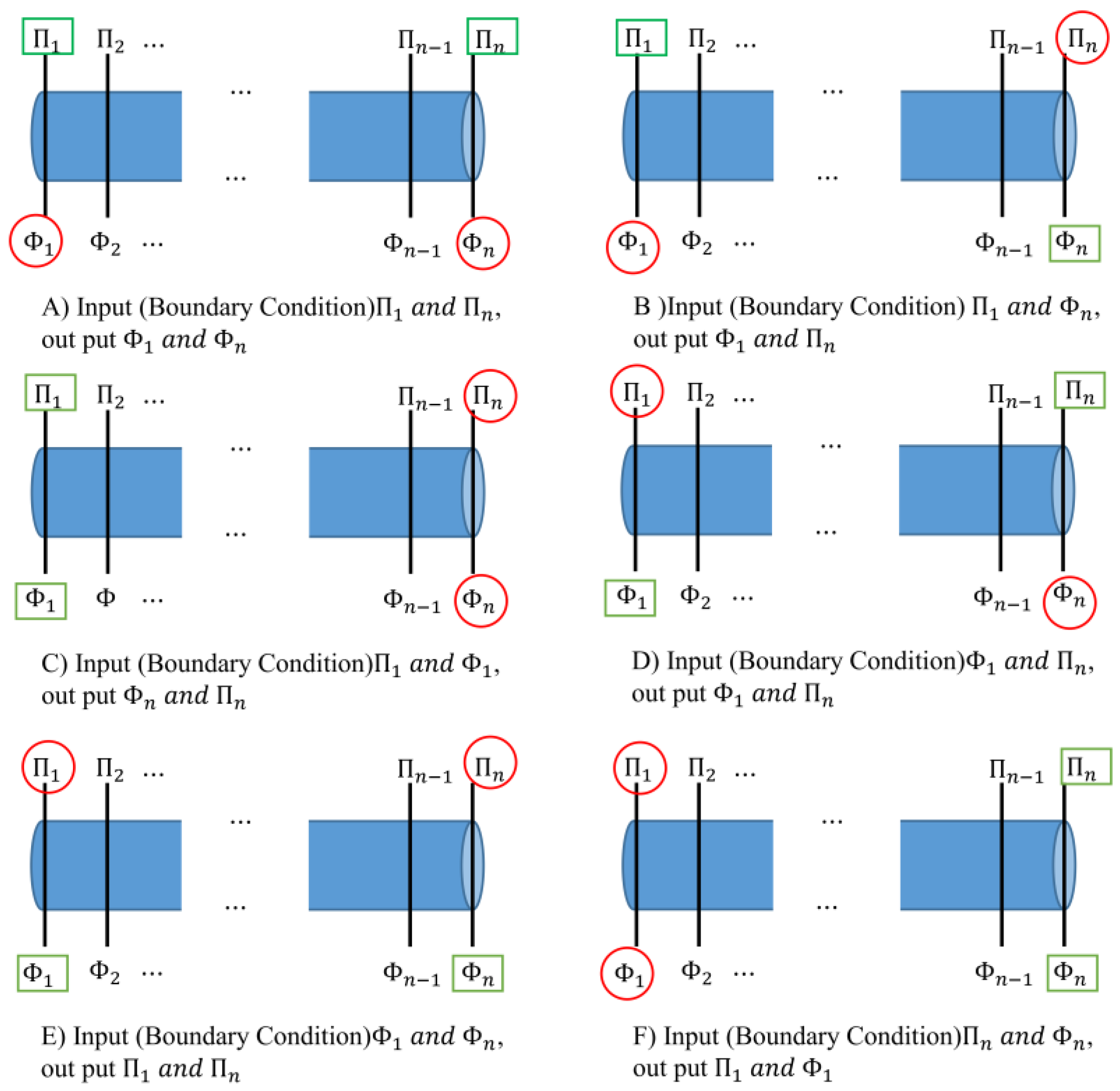
Several numerical methods are available for the solution of Ordinary differential equations (ODEs) Equations (20) and (21). Here the finite-difference approach is used for its simplicity, and because it is suitable for simulation and non-linear observer design [28]. Control variables in the different cases can be presented by the pressures head and flow rates at the beginning and end of the pipe. The solution of the discretized model, using any technique needs boundary conditions that present known values of the variables at the edge of the researched area. Boundary conditions may just be pressures head, just flows, or combining both. The selection of boundary conditions alters the construction of the models, also may change the quantity of equations wherein the discretized model is subdivided. In real systems, boundary conditions can be defined using the elements existing in the hydraulic system. Figure 3 represents the possible boundary conditions in a scheme of a discretized pipeline. We had six cases for the modelling, based on choosing the control variables.

Case 1: The controllable initial as well as boundary conditions are taken to be pressure heads at the start and ending of the pipe, see Figure 3A. The input conditions can be stated as

$$\{\begin{array}{c}\Pi \left(0,t\right)={\Pi }_{in}\left(t\right)\\ \Pi \left(L,t\right)={\Pi }_{out}\left(t\right)\end{array},$$

(22)

and output values are

$$\{\begin{array}{c}\Phi \left(0,t\right)={\Phi }_{in}\left(t\right)\\ \Phi \left(L,t\right)={\Phi }_{out}\left(t\right)\end{array}.$$

(23)

The vectors $u\left(t\right)$ and $y\left(t\right)$ are the inputs and outputs of the system respectively. We have $x={\left({\Phi }_0 {\Phi }_1 {\Phi }_{2b}{\Phi }_n{\Pi }_1{\Pi }_{2b}\gamma {\lambda \Theta }_b\right)}^T$, $u:={\left[{\Pi }_{in}{\Pi }_{out}\right]}^T={\left({\Pi }_0{\Pi }_n\right)}^T$ and $y={\left({\Phi }_0{\Phi }_n\right)}^T$. Hence,

$$\begin{array}{c}{\dot{\Phi }}_0=-\Theta g\frac{{\Pi }_1-{\Pi }_0}{\lambda }-\frac{f}{2\delta }{\Phi }_0,\\ {\dot{\Phi }}_1=-\Theta g\frac{{\Pi }_1-{\Pi }_0}{\lambda }-\frac{f}{2\delta }{\Phi }_1,\\ {\dot{\Phi }}_{2b}=-{\Theta }_{b}g\frac{\left({\Pi }_{2b}-{\Pi }_{1b}\right)}{\gamma }-\frac{f_b}{2\delta }{\Phi }_{2b},\\ {\dot{\Phi }}_n=-\Theta g\frac{\left({\Pi }_n-{\Pi }_2\right)}{\left(\Gamma -\lambda -\gamma \right)}-\frac{f}{2\delta }{\Phi }_n,\\ {\dot{\Pi }}_1=-\frac{a^2}{g\Theta }\frac{{\Phi }_1-{\Phi }_0}{\lambda },\\ {\dot{\Pi }}_{2b}=-\frac{a^2}{g{\Theta }_b}\frac{\left({\Phi }_{2b}-{\Phi }_{1b}\right)}{\gamma },\\ \dot{\gamma }=0,\\ \dot{\lambda }=0,\\ {\dot{\Theta }}_b=0,\end{array}$$

(24)

where ${\Pi }_{1b}$ and ${\Pi }_2$ are calculated using Bernoulli’s and continuity Equations as below,

$$\begin{array}{c}{\Pi }_{1b}={\Pi }_1+\eta \frac{{\Theta }_b^2{\Phi }_1^2-{\Theta }^2{\Phi }_1^2}{2g{\Theta }^2{\Theta }_b^2}.\\ {\Pi }_2={\Pi }_{2b}+\eta \frac{{\Theta }^2{\Phi }_{2b}^2-{\Theta }_b^2{\Phi }_{2b}^2}{2g{\Theta }^2{\Theta }_b^2}.\end{array}$$

(25)

Case 2: The controllable boundary conditions are taken to be flow rate and pressure head at the start and ending of the pipe, respectively, see Figure 3B. The input conditions can be stated as

$$\{\begin{array}{c}\Pi \left(0,t\right)={\Pi }_{in}\left(t\right)\\ \Phi \left(L,t\right)={\Phi }_{out}\left(t\right)\end{array},$$

(26)

and output values are

$$\{\begin{array}{c}\Phi \left(0,t\right)={\Phi }_{in}\left(t\right)\\ \Pi \left(L,t\right)={\Pi }_{out}\left(t\right)\end{array}.$$

(27)

The vectors $u\left(t\right)$ and $y\left(t\right)$ are the inputs and outputs of the system respectively. We have $x={\left({\Phi }_0{\Phi }_1 {\Phi }_{2b}{\Pi }_1{\Pi }_{2b}{\Pi }_n{\gamma \lambda \Theta }_b\right)}^T,$ $u:={\left[{\Phi }_{in}{\Pi }_{out}\right]}^T={\left({\Phi }_n{\Pi }_0\right)}^T$ and $y:={\left[{\Phi }_{in}{\Pi }_{out}\right]}^T={\left({\Phi }_0{\Pi }_n\right)}^T$. Hence,

$$\begin{array}{c}{\dot{\Phi }}_0=-\Theta g\frac{{\Pi }_1-{\Pi }_0}{\lambda }-\frac{f}{2\delta }{\Phi }_0,\\ {\dot{\Phi }}_1=-\Theta g\frac{{\Pi }_1-{\Pi }_0}{\lambda }-\frac{f}{2\delta }{\Phi }_1,\\ {\dot{\Phi }}_{2b}=-{\Theta }_{b}g\frac{\left({\Pi }_{2b}-{\Pi }_{1b}\right)}{\gamma }-\frac{f_b}{2\delta }{\Phi }_{2b},\\ {\dot{\Pi }}_1=-\frac{a^2}{g\Theta }\frac{{\Phi }_1-{\Phi }_0}{\lambda },\\ {\dot{\Pi }}_{2b}=-\frac{a^2}{g{\Theta }_b}\frac{\left({\Phi }_{2b}-{\Phi }_{1b}\right)}{\gamma },\\ {\dot{\Pi }}_n=-\frac{a^2}{g\Theta }\frac{\left({\Phi }_n-{\Phi }_2\right)}{\left(\Gamma -\lambda -\gamma \right)},\\ \dot{\gamma }=0,\\ \dot{\lambda }=0,\\ {\dot{\Theta }}_b=0,\end{array}$$

(28)

where ${\Pi }_{1b}$ and ${\Pi }_2$ are calculated using Bernoulli’s and continuity equations as below,

$$\begin{array}{c}{\Pi }_{1b}={\Pi }_1+\eta \frac{{\Theta }_b^2{\Phi }_1^2-{\Theta }^2{\Phi }_1^2}{2g{\Theta }^2{\Theta }_b^2}.\\ {\Pi }_2={\Pi }_{2b}+\eta \frac{{\Theta }^2{\Phi }_{2b}^2-{\Theta }_b^2{\Phi }_{2b}^2}{2g{\Theta }^2{\Theta }_b^2}.\end{array}$$

(29)

Case 3: The controllable initial and boundary conditions are taken to be flow rate and pressure head at the start of the pipe, see Figure 3C. The input conditions can be stated as

$$\{\begin{array}{c}\Pi \left(0,t\right)={\Pi }_{in}\left(t\right)\\ \Phi \left(0,t\right)={\Phi }_{in}\left(t\right)\end{array},$$

(30)

and output values are

$$\{\begin{array}{c}\Phi \left(L,t\right)={\Phi }_{out}\left(t\right)\\ \Pi \left(L,t\right)={\Pi }_{out}\left(t\right)\end{array}.$$

(31)

The vectors $u\left(t\right)$ and $y\left(t\right)$ are the inputs and outputs of the system respectively. We have $x={\left({\Phi }_1 {\Phi }_{2b}{\Phi }_n{\Pi }_1{\Pi }_{2b}{\Pi }_n\gamma \lambda {\Theta }_b\right)}^T$, $u:={\left[{\Phi }_{in} {\Pi }_{in}\right]}^T={\left({\Phi }_0{\Pi }_0\right)}^T$ and $y:={\left({\Phi }_n{\Pi }_n\right)}^T$. Hence,

$$\begin{array}{c}{\dot{\Phi }}_1=-\Theta g\frac{{\Pi }_1-{\Pi }_0}{\lambda }-\frac{f}{2\delta }{\Phi }_1,\\ {\dot{\Phi }}_{2b}=-{\Theta }_{b}g\frac{\left({\Pi }_{2b}-{\Pi }_{1b}\right)}{\gamma }-\frac{f_b}{2\delta }{\Phi }_{2b},\\ {\dot{\Phi }}_n=-\Theta g\frac{\left({\Pi }_n-{\Pi }_2\right)}{\left(\Gamma -\lambda -\gamma \right)}-\frac{f}{2\delta }{\Phi }_n,\\ {\dot{\Pi }}_1=-\frac{a^2}{g\Theta }\frac{{\Phi }_1-{\Phi }_0}{\lambda },\\ {\dot{\Pi }}_{2b}=-\frac{a^2}{g{\Theta }_b}\frac{\left({\Phi }_{2b}-{\Phi }_{1b}\right)}{\gamma },\\ {\dot{\Pi }}_n=-\frac{a^2}{g\Theta }\frac{\left({\Phi }_n-{\Phi }_2\right)}{\left(\Gamma -\lambda -\gamma \right)},\\ \dot{\gamma }=0,\\ \dot{\lambda }=0,\\ {\dot{\Theta }}_b=0,\end{array}$$

(32)

where ${\Pi }_{1b}$ and ${\Pi }_2$ are calculated using Bernoulli’s and continuity equations as below,

$$\begin{array}{c}{\Pi }_{1b}={\Pi }_1+\eta \frac{{\Theta }_b^2{\Phi }_1^2-{\Theta }^2{\Phi }_1^2}{2g{\Theta }^2{\Theta }_b^2}.\\ {\Pi }_2={\Pi }_{2b}+\eta \frac{{\Theta }^2{\Phi }_{2b}^2-{\Theta }_b^2{\Phi }_{2b}^2}{2g{\Theta }^2{\Theta }_b^2}.\end{array}$$

(33)

Case 4: The controllable initial and boundary conditions are taken to be flow rate at the start and pressure head at the ending of the pipe, see Figure 3D. The input conditions can be stated as

$$\{\begin{array}{c}\Pi \left(L,t\right)={\Pi }_{out}\left(t\right)\\ \Phi \left(0,t\right)={\Phi }_{in}\left(t\right)\end{array},$$

(34)

and output values are

$$\{\begin{array}{c}\Phi \left(L,t\right)={\Phi }_{out}\left(t\right)\\ \Pi \left(0,t\right)={\Pi }_{in}\left(t\right)\end{array}.$$

(35)

The vectors $u\left(t\right)$ and $y\left(t\right)$ are the inputs and outputs of the system respectively. We have $x={\left({\Phi }_1{\Phi }_{2b}{\Phi }_n{\Pi }_0{\Pi }_1{\Pi }_{2b}\gamma {\lambda \Theta }_b\right)}^T$, $u:={\left[{\Phi }_{in} {\Pi }_{out}\right]}^T={\left({\Phi }_0 {\Pi }_n\right)}^T$ and $y:={\left({\Phi }_n{\Pi }_0\right)}^T$. Hence,

$$\begin{array}{l}{\dot{\Phi }}_1=-\Theta g\frac{{\Pi }_1-{\Pi }_0}{\lambda }-\frac{f}{2\delta }{\Phi }_1,\\ {\dot{\Phi }}_{2b}=-{\Theta }_{b}g\frac{\left({\Pi }_{2b}-{\Pi }_{1b}\right)}{\gamma }-\frac{f_b}{2\delta }{\Phi }_{2b},\\ {\dot{\Phi }}_n=-\Theta g\frac{\left({\Pi }_n-{\Pi }_2\right)}{\left(\Gamma -\lambda -\gamma \right)}-\frac{f}{2\delta }{\Phi }_n,\\ {\dot{\Pi }}_0=-\frac{a^2}{g\Theta }\frac{{\Phi }_1-{\Phi }_0}{\lambda },\\ {\dot{\Pi }}_1=-\frac{a^2}{g\Theta }\frac{{\Phi }_1-{\Phi }_0}{\lambda },\\ {\dot{\Pi }}_{2b}=-\frac{a^2}{g{\Theta }_b}\frac{\left({\Phi }_{2b}-{\Phi }_{1b}\right)}{\gamma },\\ \dot{\gamma }=0,\\ \dot{\lambda }=0,\\ {\dot{\Theta }}_b=0,\end{array}$$

(36)

where ${\Pi }_{1b}$ and ${\Pi }_2$ are calculated using Bernoulli’s and continuity equations as below,

$$\begin{array}{cc}{\Pi }_{1b}={\Pi }_1+\eta \frac{{\Theta }_b^2{\Phi }_1^2-{\Theta }^2{\Phi }_1^2}{2g{\Theta }^2{\Theta }_b^2}.& \\ & {\Pi }_2={\Pi }_{2b}+\eta \frac{{\Theta }^2{\Phi }_{2b}^2-{\Theta }_b^2{\Phi }_{2b}^2}{2g{\Theta }^2{\Theta }_b^2}.\end{array}$$

(37)

Case 5: The controllable initial and boundary conditions are taken to be flow rate at the start and ending of the pipe, see Figure 3E. The input conditions can be stated as

$$\{\begin{array}{c}\Phi \left(0,t\right)={\Phi }_{in}\left(t\right)\\ \Phi \left(L,t\right)={\Phi }_{out}\left(t\right)\end{array},$$

(38)

and output values are

$$\{\begin{array}{c}\Pi \left(0,t\right)={\Pi }_{in}\left(t\right)\\ \Pi \left(L,t\right)={\Pi }_{out}\left(t\right)\end{array}.$$

(39)

The vectors $u\left(t\right)$ and $y\left(t\right)$ are the inputs and outputs of the system respectively. We have $x={\left({\Phi }_1{\Phi }_{2b}{\Pi }_0{\Pi }_1{\Pi }_{2b}{\Pi }_n\gamma {\mathrm{z}\Theta }_b\right)}^T$, $u:={\left[{\Phi }_{in}{\Phi }_{out}\right]}^T={\left({\Phi }_0{\Phi }_n\right)}^T$ and $y:={\left({\Pi }_0{\Pi }_n\right)}^T$. Hence,

$$\begin{array}{l}{\dot{\Phi }}_1=-\Theta g\frac{{\Pi }_1-{\Pi }_0}{\lambda }-\frac{f}{2\delta }{\Phi }_1,\\ {\dot{\Phi }}_{2b}=-{\Theta }_{b}g\frac{\left({\Pi }_{2b}-{\Pi }_{1b}\right)}{\gamma }-\frac{f_b}{2\delta }{\Phi }_{2b},\\ {\dot{\Pi }}_0=-\frac{a^2}{g\Theta }\frac{{\Phi }_1-{\Phi }_0}{\lambda },\\ {\dot{\Pi }}_1=-\frac{a^2}{g\Theta }\frac{{\Phi }_1-{\Phi }_0}{\lambda },\\ {\dot{\Pi }}_{2b}=-\frac{a^2}{g{\Theta }_b}\frac{\left({\Phi }_{2b}-{\Phi }_{1b}\right)}{\gamma },\\ {\dot{\Pi }}_n=-\frac{a^2}{g\Theta }\frac{\left({\Phi }_n-{\Phi }_2\right)}{\left(\Gamma -\lambda -\gamma \right)},\\ \dot{\gamma }=0,\\ \dot{\lambda }=0,\\ {\Theta }_b=0,\end{array}$$

(40)

where ${\Pi }_{1b}$ and ${\Pi }_2$ are calculated using Bernoulli’s and continuity equations as below,

$$\begin{array}{cc}{\Pi }_{1b}={\Pi }_1+\eta \frac{{\Theta }_b^2{\Phi }_1^2-{\Theta }^2{\Phi }_1^2}{2g{\Theta }^2{\Theta }_b^2}.& \\ & {\Pi }_2={\Pi }_{2b}+\eta \frac{{\Theta }^2{\Phi }_{2b}^2-{\Theta }_b^2{\Phi }_{2b}^2}{2g{\Theta }^2{\Theta }_b^2}.\end{array}$$

(41)

Case 6: The controllable boundary conditions are taken to be pressure heads and flow rate at the start and ending of the pipe, respectively, see Figure 3F. The input conditions can be stated as

$$\{\begin{array}{c}\Phi \left(L,t\right)={\Phi }_{out}\left(t\right)\\ \Pi \left(L,t\right)={\Pi }_{out}\left(t\right)\end{array},$$

(42)

and output values are

$$\{\begin{array}{c}\Phi \left(0,t\right)={\Phi }_{in}\left(t\right)\\ \Pi \left(L,t\right)={\Pi }_{in}\left(t\right)\end{array}.$$

(43)

The vectors $u\left(t\right)$ and $y\left(t\right)$ are the inputs and outputs of the system respectively. We have $x={\left({\Phi }_1{\Phi }_{2b}{\Phi }_n {\Pi }_0{\Pi }_1{\Pi }_{2b}{\gamma \lambda \Theta }_b\right)}^T$, $u:={\left[{\Phi }_{out} {\Pi }_{out}\right]}^T={\left({\Phi }_n{\Pi }_n\right)}^T$ and $y:={\left({\Phi }_0{\Pi }_0\right)}^T$. Hence,

$$\begin{array}{l}{\dot{\Phi }}_0=-\Theta g\frac{{\Pi }_1-{\Pi }_0}{\lambda }-\frac{f}{2\delta }{\Phi }_0,\\ {\dot{\Phi }}_1=-\Theta g\frac{{\Pi }_1-{\Pi }_0}{\lambda }-\frac{f}{2\delta }{\Phi }_1,\\ {\dot{\Phi }}_{2b}=-{\Theta }_{b}g\frac{\left({\Pi }_{2b}-{\Pi }_{1b}\right)}{\gamma }-\frac{f_b}{2\delta }{\Phi }_{2b},\\ {\dot{\Pi }}_0=-\frac{a^2}{g\Theta }\frac{{\Phi }_1-{\Phi }_0}{\lambda },\\ {\dot{\Pi }}_1=-\frac{a^2}{g\Theta }\frac{{\Phi }_1-{\Phi }_0}{\lambda },\\ {\dot{\Pi }}_{2b}=-\frac{a^2}{g{\Theta }_b}\frac{\left({\Phi }_{2b}-{\Phi }_{1b}\right)}{\gamma },\\ \dot{\gamma }=0,\\ \dot{\lambda }=0,\\ {\dot{\Theta }}_b=0,\end{array}$$

(44)

where ${\Pi }_{1b}$ and ${\Pi }_2$ are calculated using Bernoulli’s and continuity equations as below,

$$\begin{array}{cc}{\Pi }_{1b}={\Pi }_1+\eta \frac{{\Theta }_b^2{\Phi }_1^2-{\Theta }^2{\Phi }_1^2}{2g{\Theta }^2{\Theta }_b^2}.& \\ & {\Pi }_2={\Pi }_{2b}+\eta \frac{{\Theta }^2{\Phi }_{2b}^2-{\Theta }_b^2{\Phi }_{2b}^2}{2g{\Theta }^2{\Theta }_b^2}.\end{array}$$

(45)

4. Observer Design by Using the Extended Kalman Filter

In estimation theory, the extended Kalman filter (EKF) is the nonlinear version of the Kalman filter, which linearizes about an estimate of the current mean and covariance. The extended Kalman filter was introduced to solve the problem of non-linearity in Kalman filter. The standard extended Kalman filter is commonly derived from a first order Taylor expansion of the state dynamics and measurement model. There is a version of the extended Kalman filter that extends this concept to include also an approximation of the second order Taylor term. The extended Kalman filter resembles the Kalman filter in that they both intend to get correct first order moments. The extended Kalman filter makes the non linear function into linear function using Taylor Series, it helps in getting the linear approximation of a non linear function. However, one common idea considered in this paper for the aim of blockage identification problem is the blockage parameter approximation $\lambda , \gamma$ as well as ${\Theta }_b$, utilizing an extended Kalman filter. For this aim, the model proposed in Equations (18) and (19) has been developed by the dynamics of these parameters, also a nonlinear observer has been made for the developed system [29]. For different cases it has been assumed to measure only pressures head, or only flow rates or combination of both at the beginning or end of the pipeline. For case 1, flow rates at the start and ending of the pipe are considered as outputs which are directly measured as follows,

$$y={\left[{\Phi }_0 {\Phi }_n\right]}^T,$$

(46)

and the pressure heads at the start and ending of the pipe considered as known inputs are

$$u={\left[{\Pi }_0 {\Pi }_n\right]}^T.$$

(47)

Also,

$$\dot{\lambda }=0; \dot{\gamma }=0; {\dot{\Theta }}_b=0.$$

(48)

The derivatives of blockage parameters $z, \lambda$ and ${\Theta }_b$ have been taken zero as their alterations are minute. Therefore Equations (18) and (19) can be extended as below,

$$\left[\begin{array}{c}{\dot{\Phi }}_0\\ {\dot{\Phi }}_1\\ {\dot{\Phi }}_{2b}\\ {\dot{\Phi }}_n\\ {\dot{\Pi }}_1\\ {\dot{\Pi }}_{2b}\\ \dot{\gamma }\\ \dot{\lambda }\\ {\dot{\Theta }}_b\end{array}\right]=\left[\begin{array}{c}-\Theta g\frac{{\Pi }_1-{\Pi }_0}{\lambda }-\frac{f}{2\delta }{\Phi }_0\\ -\Theta g\frac{{\Pi }_1-H_0}{\lambda }-\frac{f}{2\delta }{\Phi }_1\\ -{\Theta }_{b}g\frac{({\Pi }_{2b}-{\Pi }_{1b})}{\gamma }-\frac{f_b}{2\delta }{\Phi }_{2b}\\ -Ag\frac{({\Pi }_n-H_2)}{(L-\lambda -\gamma )}-\frac{f}{2\delta }{\Phi }_n\\ -\frac{a^2}{g\Theta }\frac{{\Phi }_1-{\Phi }_0}{\lambda }\\ -\frac{a^2}{g{\Theta }_b}\frac{({\Phi }_{2b}-{\Phi }_{1b})}{\gamma }\\ 0\\ 0\\ 0\end{array}\right],$$

(49)

where ${\Pi }_{1b}$ and ${\Pi }_2$ are computed as below [27],

$$\begin{array}{cc}{\Pi }_{1b}={\Pi }_1+\eta \frac{{\Theta }_b^2{\Phi }_1^2-{\Theta }^2{\Phi }_1^2}{2g{\Theta }^2{\Theta }_b^2}.& \\ & {\Pi }_2={\Pi }_{2b}+\eta \frac{{\Theta }^2{\Phi }_{2b}^2-{\Theta }_b^2{\Phi }_{2b}^2}{2g{\Theta }^2{\Theta }_b^2}.\end{array}$$

(50)

Accordingly, Equation (49) can be formulated as below,

$$\dot{x}=\varphi \left(x,u\right),$$

(51)

where $x={\left({\Phi }_1{\Phi }_{2b}{\Phi }_n{\Pi }_0{\Pi }_1{\Pi }_{2b}\gamma \lambda {\Theta }_b\right)}^T$ and $\varphi \left(x,u\right)$ is taken as a nonlinear function.

Now, to estimate the block parameters $\lambda , \gamma$ and $A_0$, a discrete-time extended Kalman filter is designed for the nonlinear model described in Equation (49). To do that, this model is discretized by using Heun’s method. In this method, the solution for the initial value problem is given by [30],

$$\begin{array}{c}\dot{x}=\varphi \left(x\left(t\right),u\left(t\right)\right),\\ x\left(t_0\right)= x_0.\end{array}$$

(52)

Therefore,

$$x^{i+1}=x^i+\frac{\Delta t}{2}\left[\varphi \left(x^i,u^i\right)+\varphi \left(x^i+\Delta t\varphi \left(x^i,u^i\right),u^{i+1}\right)\right],$$

(53)

where $\Delta t$ is taken to be the time step also, $i$ is taken to be the index of discrete-time. Applying Equation (53) into Equation (49) the following are extracted,

$$\begin{array}{l}{\Phi }_0^{i+1}={\Phi }_0^i+\frac{\Delta t}{2}(-\Theta g\frac{{\Pi }_1^i-{\Pi }_0^i}{z^i}-\frac{f}{2\delta }{\Phi }_0^i-\Theta g\frac{{\hat{\Pi }}_1^{i+1}-{\Pi }_0^{i+1}}{z^{i+1}})-\frac{f}{2\delta }{\hat{\Phi }}_0^{i+1},\\ {\Phi }_1^{i+1}={\Phi }_1^i+\frac{\Delta t}{2}(-Ag\frac{{\Pi }_1^i-{\Pi }_0^i}{z^i}-\frac{f}{2\delta }{\Phi }_1^i-Ag\frac{{\hat{\Pi }}_1^{i+1}-{\Pi }_0^{i+1}}{z^{i+1}})-\frac{f}{2\delta }{\hat{\Phi }}_1^{i+1},\\ {\Phi }_{2b}^{i+1}={\Phi }_{2b}^i+\frac{\Delta t}{2}(-{\Theta }_{b}g\frac{{\hat{\Pi }}_{2b}^i-{\hat{\Pi }}_{1b}^i}{{\lambda }^i}-\frac{f_b}{2\delta }{\Phi }_{2b}^i-Ag\frac{{\hat{\Pi }}_{2b}^{i+1}-{\hat{\Pi }}_{1b}^{i+1}}{{\gamma }^{i+1}})-\frac{f}{2\delta }{\hat{\Phi }}_{2b}^{i+1},\\ {\Phi }_n^{i+1}={\Phi }_n^i+\frac{\Delta t}{2}(-\Theta g\frac{{\hat{\Pi }}_n^i-{\hat{\Pi }}_2^i}{(\Gamma -{\lambda }^i-{\gamma }^i)}-\frac{f}{2\delta }{\Phi }_n^i-Ag\frac{{\hat{\Pi }}_n^{i+1}-{\hat{\Pi }}_2^{i+1}}{(\Gamma -{\lambda }^{i+1}-{\gamma }^{i+1})})-\frac{f}{2\delta }{\hat{\Phi }}_n^{i+1},\\ {\Pi }_1^{i+1}={\Pi }_n^i+\frac{\Delta t}{2}(-\frac{a^2}{g\Theta }\frac{{\Phi }_1^i-{\Phi }_0^i}{{\lambda }^i}-\frac{a^2}{g\Theta }\frac{{\hat{\Phi }}_1^{i+1}-{\hat{\Phi }}_0^{i+1}}{{\lambda }^{i+1}}),\\ {\Pi }_{2b}^{i+1}={\Pi }_{2b}^i+\frac{\Delta t}{2}(-\frac{a^2}{g{A}_b}\frac{{\Phi }_1^i-{\Phi }_0^i}{{\gamma }^i}-\frac{a^2}{g\Theta }\frac{{\hat{\Phi }}_1^{i+1}-{\hat{\Phi }}_0^{i+1}}{{\lambda }^{i+1}}),\\ {\gamma }_{}^{i+1}={\gamma }^i,\\ {\lambda }_{}^{i+1}={\lambda }^i,\\ {\Theta }_b{}_{}^{i+1}={\Theta }_b{}^i,\end{array}$$

(54)

in compact form:

$$x^{i+1}=\varphi \left(x^i,u^{i+1},u^i\right); y^i=H{x}^i.$$

(55)

where

$$\begin{array}{c}{x}^i={\left[{\Phi }_0^i {\Phi }_1^i {\Phi }_{2b}^i {\Phi }_n^i {\Pi }_n^i {\Pi }_{2b}^i {\gamma }^i {\lambda }^i {\Theta }_b{}^i\right]}^T ;\\ u^i={\left[{\Pi }_0^i {\Pi }_n^i\right]}^T\\ \mathrm{H}=\left[\begin{array}{ccc}1& 0& \begin{array}{ccc}0& \begin{array}{ccc}0& 0& 0\end{array}& \begin{array}{ccc}0& 0& 0\end{array}\end{array}\\ 0& 0& \begin{array}{ccc}0& \begin{array}{ccc}1& 0& 0\end{array}& \begin{array}{ccc}0& 0& 0\end{array}\end{array}\end{array}\right].\end{array}$$

(56)

Observer Approach

A the discrete-time extended Kalman filter as a state observer for the system Equation (49) is defined as below [31],

$${\widehat{x}}^i={\widehat{x}}^{\tilde{i}}+{\kappa }^i(y^i-H{\widehat{x}}^{\tilde{i}}),$$

(57)

where ${\widehat{x}}^{\tilde{i}}$ is the priori estimate of $x^i$:

$${\widehat{x}}^{\tilde{i}}=\varphi ({\widehat{x}}^{i-1},u^{i-1}).$$

(58)

${\kappa }^i$ is the Kalman gain:

$${\kappa }^i=P^{\tilde{i}}{H}^T{(H{P}^{\tilde{i}}{H}^T+R)}^{-1}.$$

(59)

$P^{\tilde{i}}$ is the priori covariance matrix:

$$P^{\tilde{i}}=J^i{P}^{i-1}{\left(J^i\right)}^T+Q.$$

(60)

$P^i$ is the posteriori covariance matrix:

$$P^i=\left(I-K^{i}H\right)P^{\tilde{i}}.$$

(61)

$J^i$ is the Jacobian matrix:

$$J^i=\frac{\partial \varphi \left(x,u\right)}{\partial x}|{}_{x={\widehat{x}}^i}.$$

(62)

Finally, $R$ and $Q$ are known as the covariance matrices of measure and process noises, respectively. Notice that:

$${\widehat{x}}^i=({\widehat{\Phi }}_1^i {\widehat{\Phi }}_{2b}^i {\widehat{\Phi }}_n^i {\widehat{\Pi }}_0^i {\widehat{\Pi }}_1^i {\widehat{\Pi }}_{2b}^i {\widehat{\gamma }}_{}^i {\widehat{\lambda }}_{}^i {\widehat{\Theta }}_b^i),$$

(63)

with $P^{\tilde{0}}={(P^{\tilde{0}})}^T>0, R=R^T>0$ and $Q=Q^T>0$.

5. Simulation Results

Here, simulations were carried out in Matlab for one case for the model shown in Figure 1. The model was realized on the pipeline with the following physical parameters:

The length of the pipeline was Γ $=120\mathrm{m}$, the diameter of the pipe was δ $=0.08\mathrm{m}$, the cross-section was Θ $=5.03\times {10}^{-3}{\mathrm{m}}^2$, density was $\rho =1000\mathrm{kg}/{\mathrm{m}}^3,$ gravity was $g=9.81\mathrm{m}/{\mathrm{s}}^2$, the friction factor of the pipe was $f=0.006$, the friction factor of the blockage part was $f_b=0.016$ and the wave speed was $a=1250\mathrm{m}/\mathrm{s}$.

Control variables are the pressures head at the start and ending of the pipeline (${\Pi }_0$ and ${\Pi }_n$). In addition, the flow rates (${\Phi }_0$ and ${\Phi }_n$) are taken to be outputs of the system.

The covariance matrices of measure and process noises introduced by expressions respectively

$$\check{R}=\mathrm{Diagonal}\mathrm{Matrix}\left[2.25\times {10}^{-5},5.5\times {10}^{-2},2.25\times {10}^{-5},1000,{10}^{-7}\right]$$

(64)

$$\check{Q}=\mathrm{Diagonal}\mathrm{Matrix}\left[2.25\times {10}^{-5},2.25\times {10}^{-5}\right]$$

(65)

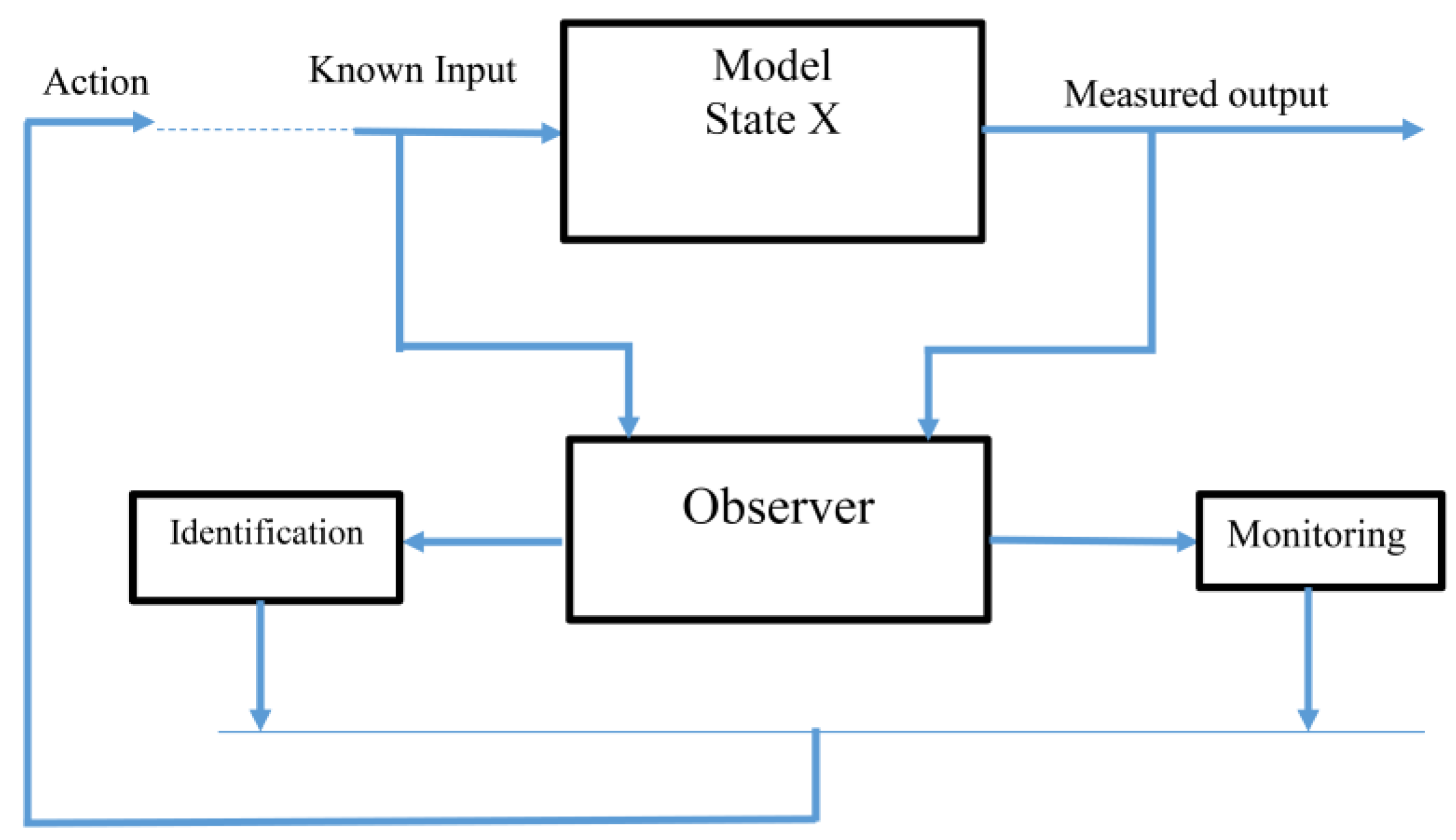
The initialization of the state is given in

Table 1. Initialization second order extended Kalman filter (SEKF).

CEKF	Value	Units
${\hat{\Phi }}_1$	$7.75 \times {10}^{-3}$	$({\mathrm{m}}^3/\mathrm{s})$
${\hat{\Pi }}_{leak}$	$8.32$	$(\mathrm{m})$
${\hat{\Phi }}_2$	$7.75 \times {10}^{-3}$	$({\mathrm{m}}^3/\mathrm{s})$
$\widehat{\lambda }$	$45.42$	$(\mathrm{m})$
$\hat{\gamma }$	0	$({\mathrm{m}}^{\frac{5}{2}}/\mathrm{s})$

. The model, the observer, as well as the state feedback construction are demonstrated in Figure 4.

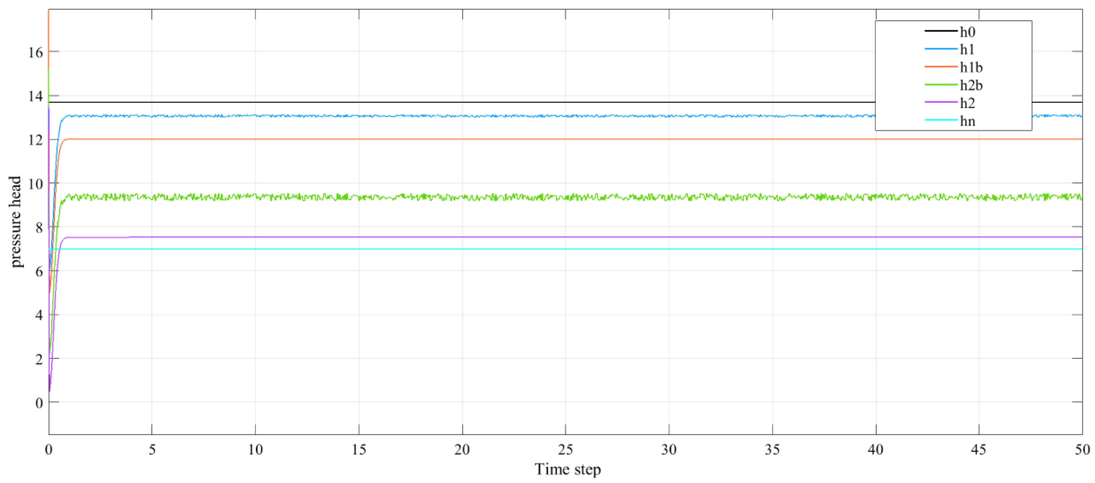
Figure 4 and Figure 5 demonstrate the simulated pressure head at the inlet $\left(H\left(in\right)=H_0=14 \mathrm{m}\right)$ and outlet $\left(H\left(out\right)=H_n=7.3 \mathrm{m}\right)$ of the pipe.

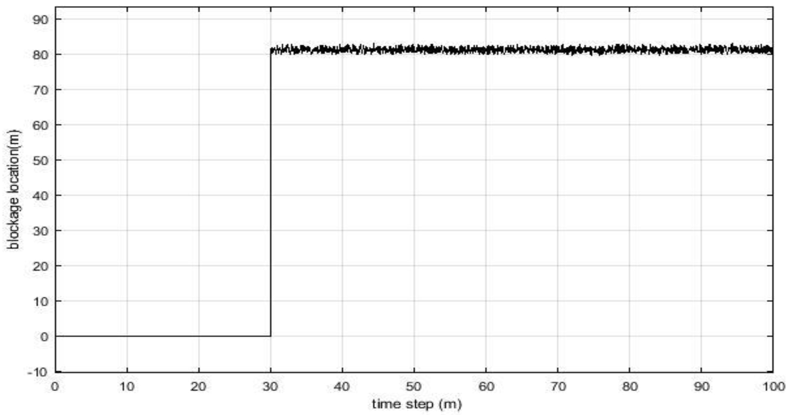
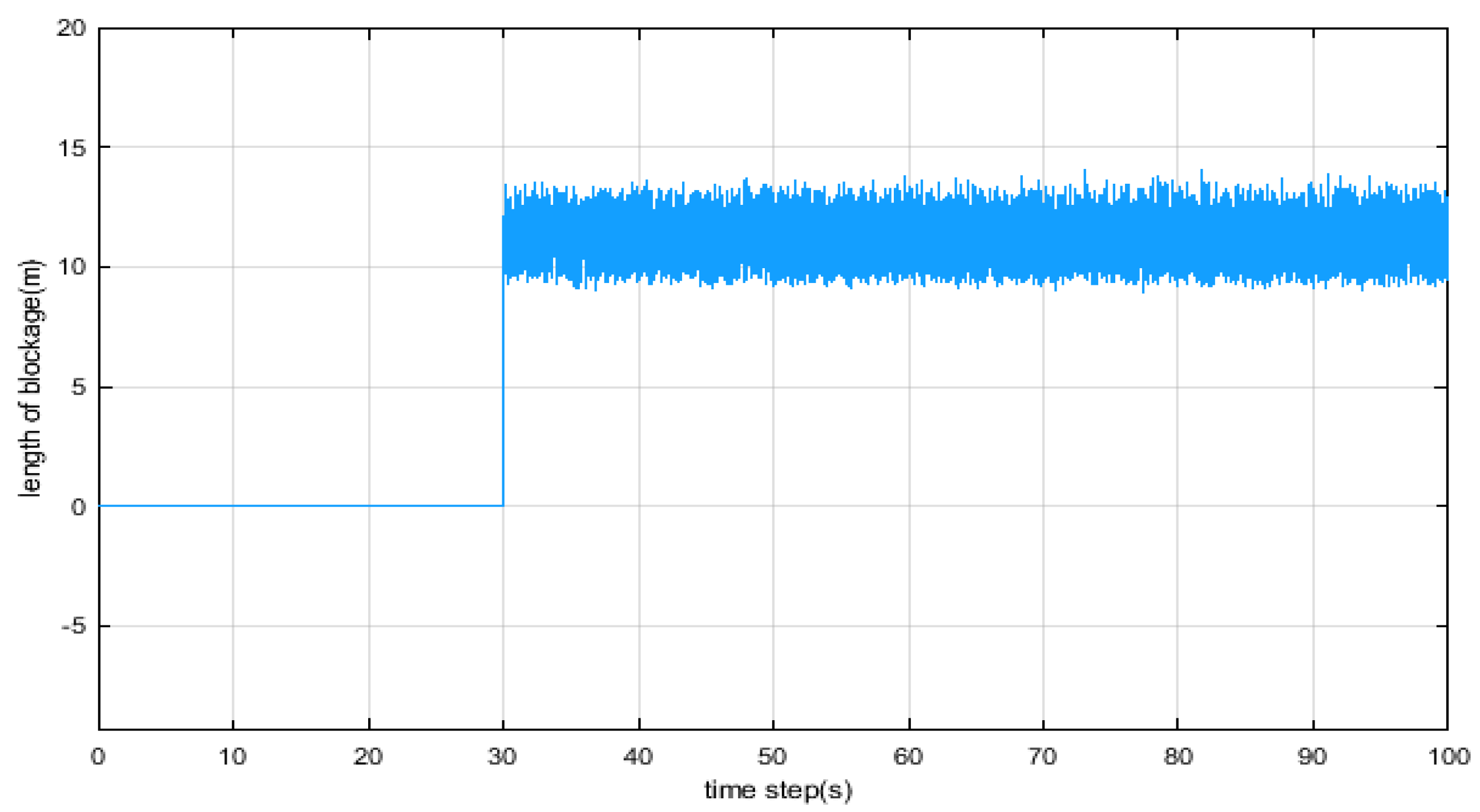
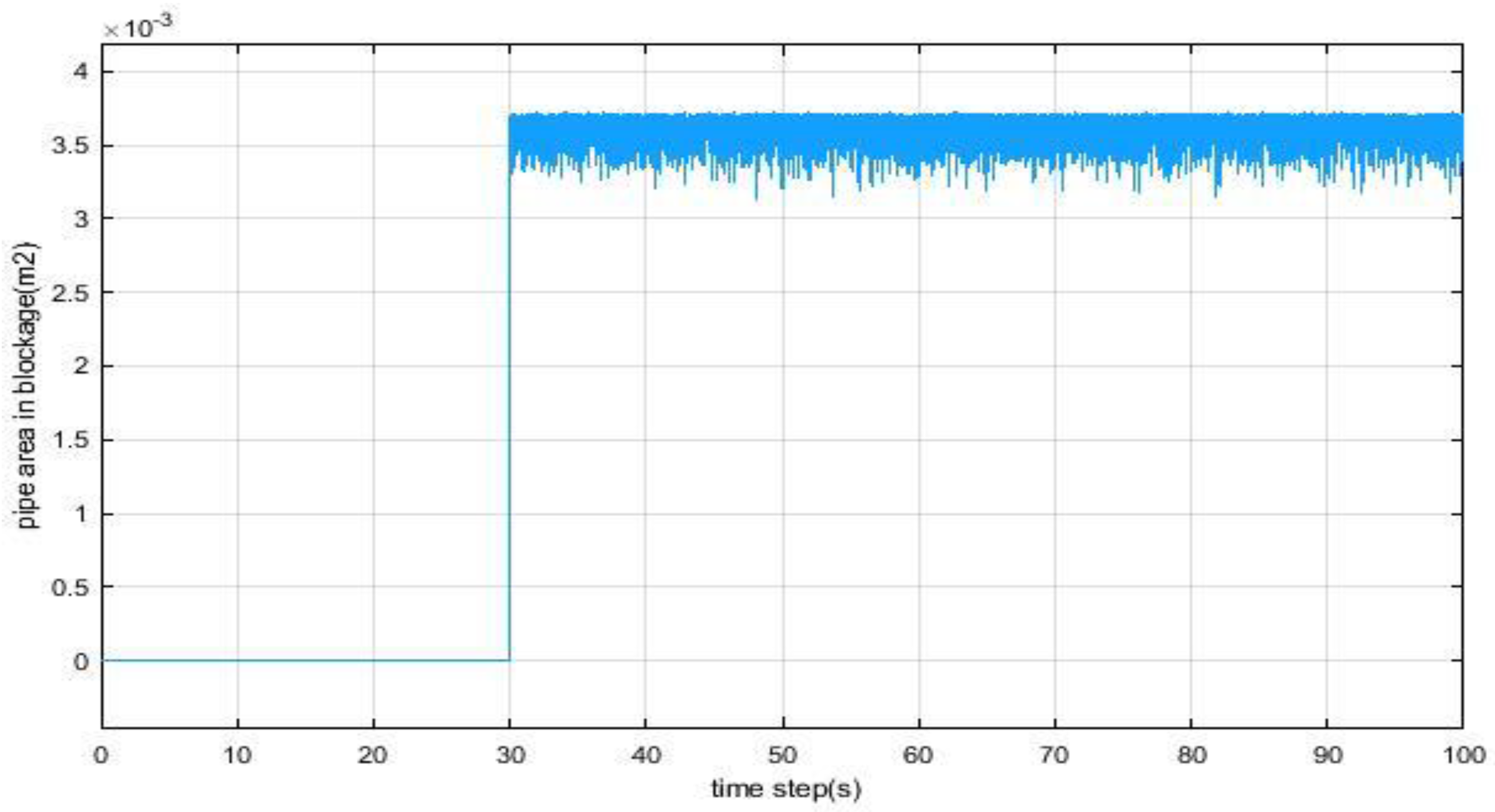
Figure 6, Figure 7 and Figure 8 shows the estimation of the position, length and the area of blockage in the pipeline. Where the Position of blockage was 80 m from initial of pipe and length of blockage was 12.2 m and cross section area in blockage was $3.5 \times {10}^{-3} {\mathrm{m}}^2$.

6. Conclusions

The second order extended Kalman filter (SEKF) is based on a second order Taylor expansion of a nonlinear system, in contrast to the more common (first order) extended Kalman filter (EKF) that is based on a second order Taylor expansion of a nonlinear system. The objective of this paper was to analyse and model the blockage in the pipe networks. We utilized the finite difference technique since it is an uncomplicated approach for designing a more appropriate model for observing and controlling the construction of the nonlinear system. This technique partitions the whole pipe into $N$ sectors. Flow and pressure head estimations were well estimated in the presence of a blockage. Some theorems were presented in order to detect blockage in the system. In future we will investigate the estimation of multi blockages in the pipe networks.