Single Residential Load Forecasting Using Deep Learning and Image Encoding Techniques

Abstract

The integration of more renewable energy resources into distribution networks makes the operation of these systems more challenging compared to the traditional passive networks. This is mainly due to the intermittent behavior of most renewable resources such as solar and wind generation. There are many different solutions being developed to make systems flexible such as energy storage or demand response. In the context of demand response, a key factor is to estimate the amount of load over time properly to better manage the demand side. There are many different forecasting methods, but the most accurate solutions are mainly found for the prediction of aggregated loads at the substation or building levels. However, more effective demand response from the residential side requires prediction of energy consumption at every single household level. The accuracy of forecasting loads at this level is often lower with the existing methods as the volatility of single residential loads is very high. In this paper, we present a hybrid method based on time series image encoding techniques and a convolutional neural network. The results of the forecasting of a real residential customer using different encoding techniques are compared with some other existing forecasting methods including SVM, ANN, and CNN. Without CNN, the lowest mean absolute percentage of error (MAPE) for a 15 min forecast is above 20%, while with existing CNN, directly applied to time series, an MAPE of around 18% could be achieved. We find the best image encoding technique for time series, which could result in higher accuracy of forecasting using CNN, an MAPE of around 12%.

1. Introduction

In power systems, the whole energy production within a period of time should be always equal to the whole energy consumption, whether consumed in loads or lost in carrier assets like transmission lines [1]. In any conditions that this balance is not met for a while, the system would face security challenges or even collapse [2,3]. There are two types of variables in the system, controllable and uncontrollable parameters. The latter brings uncertainty to the system, which makes the operation and control challenging [4]. High voltage (HV) transmission systems have many established control strategies to ensure power balance and normal operation. These strategies are mainly applied by means of big power plants, which are capable of performing load frequency control. The amount of demand is also forecast to provide an input for proper power dispatching.

Forecasting electricity demand is performed in different time horizons: short, medium, and long term load forecasting. Figure 1 classifies load forecasting into different types from the time horizon perspective and geographic area or level aspect. Methods for medium or long term load forecasting can be classified into two types of models as end-use models and econometric models. The former collects statistical aggregated data of electricity demand from residential, commercial, and industrial sectors and explains energy demand as a function of the number of consumers in the market. The latter model estimates the relationship between the energy consumption and the economic factors that influence the energy consumption, and it combines economic theory and statistical techniques (e.g., linear regression or time series methods) [5].

Short term load forecasting (STLF) has been used since 1920 mainly for the daily energy supply routine [6]. It is needed for economic energy dispatch, unit commitment, and energy trade in the competitive market. The time horizon for STLF varies from intervals within the next hour, day-ahead, or one week.

There are many different forecasting algorithms that can predict demand at the transmission level with a very high accuracy. This is mainly for two reasons; firstly, the loads at this level have a large amount of aggregated values with slow changes, secondly, the loads are the demand of distribution grids that are mostly passive networks with a low level of distributed generation (DG). However, the integration of DG, especially from intermittent renewable resources, makes forecasting challenging.

The main reason that the variable renewable energy (VRE) has the potential to create operational challenges in the system is its variability. This may even result in low probability, but high impact events in power systems. The intermittent behavior of VREs like wind generation or solar production brings uncertainty for the power system, as the predictability of such generation is quite low.

As VRE generators are either uncontrollable or difficult to control promptly, it is necessary to exploit the flexibility provided by storage systems [7], another vector of energy like district heating or gas network, and the demand side. Otherwise, distributed generations may need to be curtailed or the distribution network would demand more power beyond the scheduled profile. As a less costly solution, demand side management (DSM) is attracting attention, and it is becoming a more common energy management paradigm.

In this regard, we address a very important prerequisite of demand response (DR) as a class of DSM mechanisms, which is load prediction; in order to intelligently and efficiently set the input parameters of DR, we need to have an estimation of load behavior.

Considering the importance of DR and the share of residential loads in distribution system demand, we aim at studying forecasting solutions for single residential loads. Reviewing the literature, it is found that there are not very accurate solutions to forecast such loads or the methods are not as developed as those applied to aggregated loads like buildings or at higher voltage levels like substations.

Within the context of load forecasting of single households with high volatility, we propose the integration of time series with image encoding methods into a convolutional neural network (CNN). As per forecasting, time series are currently fed to CNN directly, which implies a one-directional first layer. In our proposed method, image encoding techniques would make the first layer two-dimensional (2D), which demonstrates a higher accuracy. We apply three different image encoding methods to time series of historic load data including the recurrence plot, Gramian angular field, and Markov transition field. We introduce the one with the higher accuracy in the case of integration into CNN. This is not only a new contribution to the limited number of existing methods of single residential load forecasting, but also improves the accuracy of load forecasting of such small scale volatile loads.

Experiments on the load dataset confirm the improvement in the forecasting results. In comparison with other well established methods, Support Vector Machines (SVM) [8], Artificial Neural Network (ANN) [9], and 1D-CNN [10], the proposed method gives more accurate values.

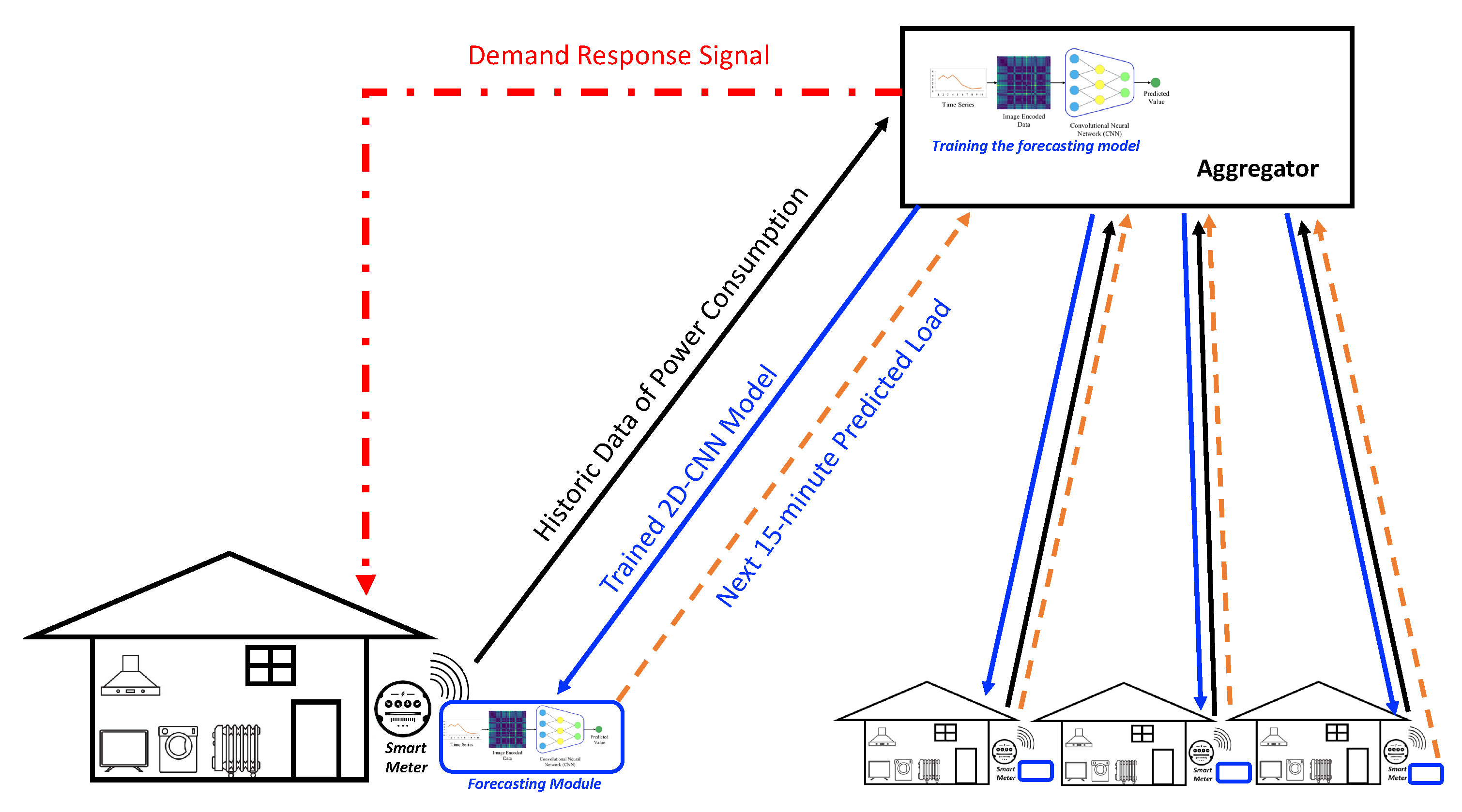
Figure 2 illustrates a high level scheme of the application of single residential load forecasting in demand response; once historic data of load power consumption (e.g., two year data) are collected, the model can be trained at the aggregator or an agent’s server. The trained model/algorithm can be embedded in a smart home to predict the next 15 min of load using the previous 24 h of measured consumption. This predicted value can be used by the aggregator to set appropriate demand response signals to be sent to the smart home for possible actions on smart appliances.

The rest of this paper contains the following sections: Section 2 reviews the impacts of renewable energy integration into distribution systems and the increasing need to estimate the load to manage the demand side. A literature review of load forecasting methods, especially those that predict residential loads, is presented in this section. In Section 3, some different image encoding techniques applied to time series, as well as the deep learning model are introduced, and the methodology of our proposed solution is presented. To evaluate the performance of the new solution, we applied it to a well known Boston housing dataset and a set of historic data of active power consumption of a single residential household. In Section 4, the performance of our proposed solution is compared with three existing methods, and in Section 5, the paper is concluded with some short remarks.

2. Background

In this section, the impacts of variable renewable resources are detailed, the importance of demand response is briefly introduced, and the contribution of load forecasting in demand response is discussed. Some existing load forecasting methods are then presented to address the current gap in the field.

2.1. Renewable Energy Integration

Integration of intermittent renewable energy resources as distributed generation in distribution systems has shifted these systems from a passive paradigm to active networks [7]. The demand from the HV system perspective is no longer pure loads at consumption centers and distribution networks. It is actually the net demand, which is the difference between consumption and local distributed generation. Considering variable renewable energy (VRE) resources as distributed generation, the net consumption would have higher uncertainty and hence be more difficult to forecast. It also becomes more crucial to predict such demands as any dramatic changes in environmental conditions like solar irradiation, weather, temperature, and wind speed would change the net demand profile very fast, which may not be captured promptly by system control and management systems. This could result in power imbalance [11], low power quality, or voltage violations. If a similar scenario occurs in neighboring distribution networks, the aggregation of effects would even initiate some frequency deviation in the upstream transmission systems.

For the VREs with a very limited reactive control, such as fixed speed induction wind turbines or small PV inverters, a lack of reactive power also increases voltage instability [12]. This occurs because of the variations of wind speed and the irregular solar radiation with time.

In the transient or short term, from milliseconds to seconds, high penetration of VREs would also present challenges for system stability. For the renewable energy sources with a very limited reactive control, such as fixed speed induction wind turbines or small PV inverters, a lack of reactive power increases voltage instability. This occurs because of the variations of wind speed and the irregular solar radiation with time. Voltage fluctuation can make problems for the sensitive electric and electronic devices and can decrease their useful life time.

VREs can also impact system voltage indirectly: electronic devices and non-linear appliances usually inject harmonics to the network, which are minimized by current control systems on conventional power generators, while VREs’ incapability of absorbing such harmonics can potentially cause voltage distortion [13]. From the other side, active power control is not widely used by wind and solar generators currently, and this diminishes system inertia. Low inertia consequently results in frequency control deterioration and eventually frequency instability. In the large bulk power plants, the rotating inertia reduces fluctuations in case there are disturbances to the grid; however, VRE generators have a low frequency response capability and, in some cases like PV, no inertia, as well as no frequency response is provided.

In the medium term, from some minutes to days, power system balance is threatened by the increasing share of VRE. If system flexibility is low and there is no ramping reserve from generators, any dramatic changes in weather conditions would lead to power imbalances by VREs. High penetration of VRE increases the need for greater flexibility in the rest of the system to allow economic dispatch. This is because overcoming the uncertainty of the net load (total load minus production of VRE) requires more load following reserves due to the low predictability of VREs’ output.

In long term planning, months to some years, the adequacy becomes challenging. Maximum generation of VRE does not necessarily match peak demand periods, and it even often occurs during periods of relatively low demand, which can cause over-generation. System adequacy is also affected by the location dependency of VRE since the best places for wind or solar power production may be located far from the load centers and even existing transmission lines. This can cause grid congestions. When dispatchable generation is replaced with high amount of VREs, system reliability will also be affected in the long term [14]. Moreover, encouraging investors with incentives and the capacity market mechanism brings new challenges as conventional high cost generators will gradually lose their attraction.

2.2. Demand Response

Demand side management applies some mechanisms to change the load profile of customers, aligning it with the generation power profile. These actions may shift or shave load curves either directly or through sending suggestion signals to consumers.

Demand response (DR) is a class of DSM mechanisms that reschedules users’ energy pattern usage according to the responses to electricity price or the incentives of the power utility [15]. DR keeps consumer in the loop and makes them aware of energy issues. DR benefits customers, the utility, and also society. Customer benefits include electricity demand satisfaction, reducing electricity bills, improving the life cycle of equipment and productivity. Some of the benefits for utilities are lowering the cost of services, improving the operating efficiency and flexibility, and improving customer service. Societal benefits mainly include environmental degradation reduction and resource conservation.

In [16,17], incentive based and price based DR schemes were discussed. In [18], incentive based schemes were recommended as more effective solutions for demand peak shaving, and the work in [19] showed how customers would be encouraged to participate in load shifting by means of rewards and how this could eventually lead to voltage profile improvement.

In the DR process, the system operator has low or no information about the load characteristics or operating regime of the appliances, especially for domestic and thermoelectric devices. Therefore, it needs to forecast the loads for the time of response so that it can make optimal decisions to control or shift the energy of appliances.

In order to set the input parameters of DR intelligently and efficiently, we need to have an estimation of the load behavior. This implies the necessity of predicting the load consumption during time to support adjusting incentives or tariffs [20,21].

2.3. Load Forecasting in Distribution Systems

Some of the different existing methods that have already been applied to forecast electric loads are reviewed in this subsection. Some methods are intended to forecast loads at aggregated levels like the substation or building levels, while some methods try to capture the consumption behavior of single customers. There are also methods to predict the consumption behavior of single appliances like air conditioners or highly demanding electric loads in distribution systems such as heat pumps.

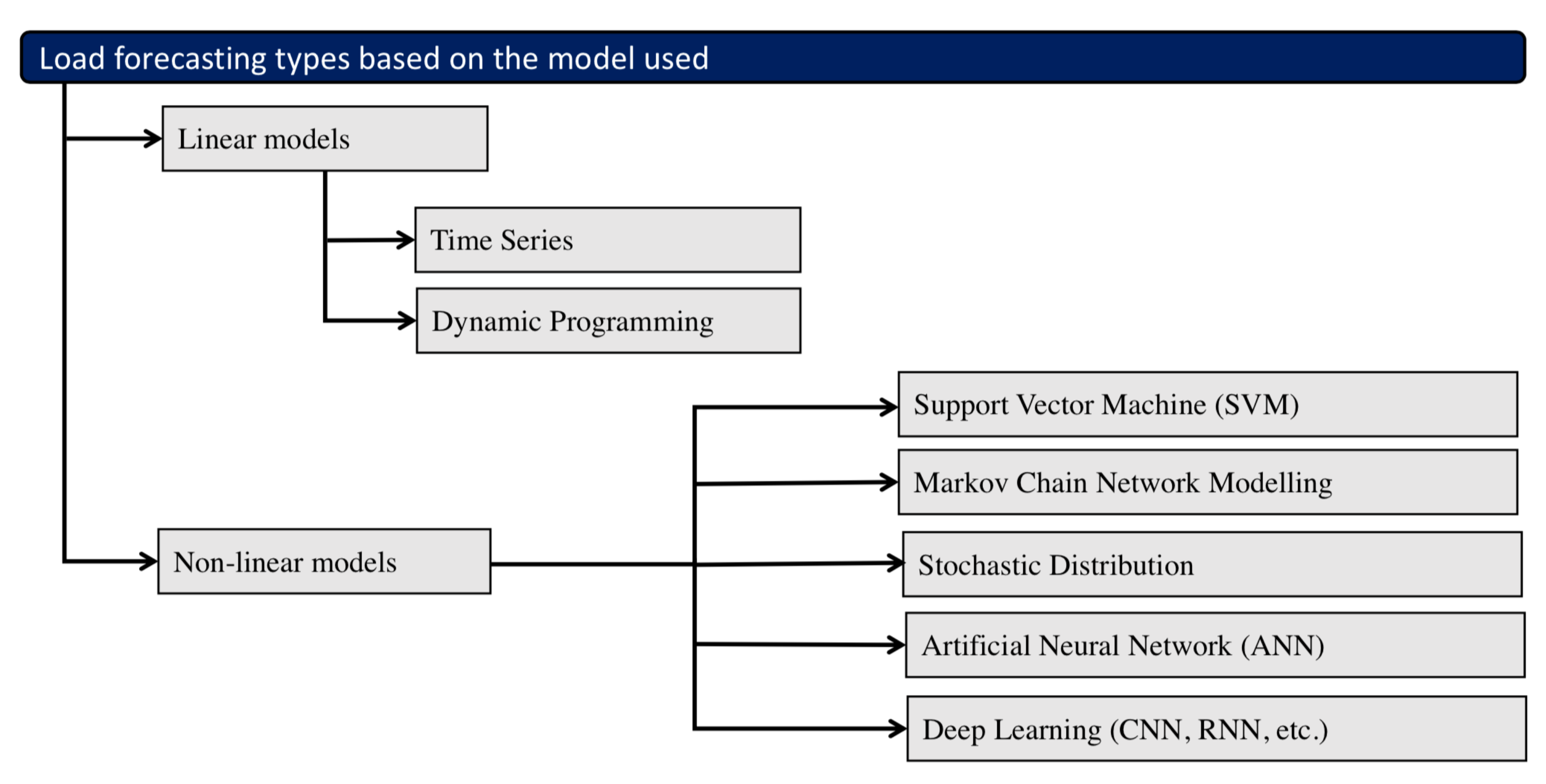
Figure 3 summarizes different types of models and algorithms used in load forecasting. The authors in [22,23] proposed some accurate methods to forecast aggregated loads at the substation level. The work in [24] presented some algorithms based on machine learning to improve the forecasting accuracy of the aggregated loads. In [25], the authors proposed a new approach to load forecasting in the presence of active demand, based on a decomposition of the load into its components. In this study, the aggregated load of about 60 consumers from an Italian LV network was used to demonstrate the performance of the proposed approach. The work in [26] presented a probabilistic load forecasting model in which weather forecasting uncertainty was used. The artificial neural network (ANN) and the probabilistic temperature forecasts were used to build this probabilistic normal load forecasting model. Although this model could achieve satisfactory performance with a low average mean absolute percentage error, it was developed to forecast loads at the building level including several customers. The work in [27] also presented a more accurate method based on deep learning algorithms for day-ahead building level load forecasts.

There are also some forecasting methods that aim to predict the consumption of large appliances or high consumption devices like boilers for district heating systems [28], heat pumps [29], electric vehicles at the station columns [30], etc. Different methods have been introduced in the literature for improving the accuracy of the load forecasting of single devices: data partitioning techniques in [31], or machine learning techniques, probability theory, and statistics in [29] for the prediction of electricity load consumption of heat pumps.

Considering the importance of DR and the share of residential loads in distribution system demand, we aim at studying forecasting solutions for single residential loads. There are many appliances at the household level whose load would be managed if it were predictable. This not only benefits system operators, but also adds value to home energy management systems, user awareness applications, and non-intrusive load monitoring (NILM) algorithms [32].

Reviewing the literature shows a limited number of contributions in proposing advanced methods for single residential load forecasting. The accuracy of the existing methods applied to single loads are also low compared to the ones applied to the aggregated loads. This is actually due to the high volatility of single residential loads; a few home appliances with different duty cycles whose switching would suddenly jump up or down the load profile. Switching on an electric oven or a dishwasher may increase the total load from 30% to 70% of the rated power. The load volatility of residential customers has an inverse correlation with the number of appliances of the household.

The fewer the appliances, the higher the volatility in the load curve could be expected, and this makes forecasting more difficult.

In [33], the authors described the accuracy of load forecasting at different levels of aggregation. They showed that aggregation of loads would improve the short term forecasting, although the performance improved until a point beyond which no further improvement could be seen. This study proved that short term load forecasting of single loads, for example a household demand, was much more difficult than predicting the consumption of a residential building with several households.

The authors in [34,35] used deep learning techniques to forecast single residential loads. The former extended a load forecasting approach based on deep long short term memory (LSTM) with automatic hyperparameter tuning to cope with the high volatility of single loads. The latter, instead, presented an LSTM recurrent neural network (RNN) method to improve the accuracy of single load forecasting.

The authors in [36] proposed a method based on support vector regression (SVR) modeling to forecast the energy consumption of single residential customers. The data granularity in their study was daily and hourly, and the performance of the model in terms of accuracy was quite low: the lowest mean absolute percentage of error (MAPE) was 12.78% for daily forecast and 23.31% for hourly forecast.

3. Methodology

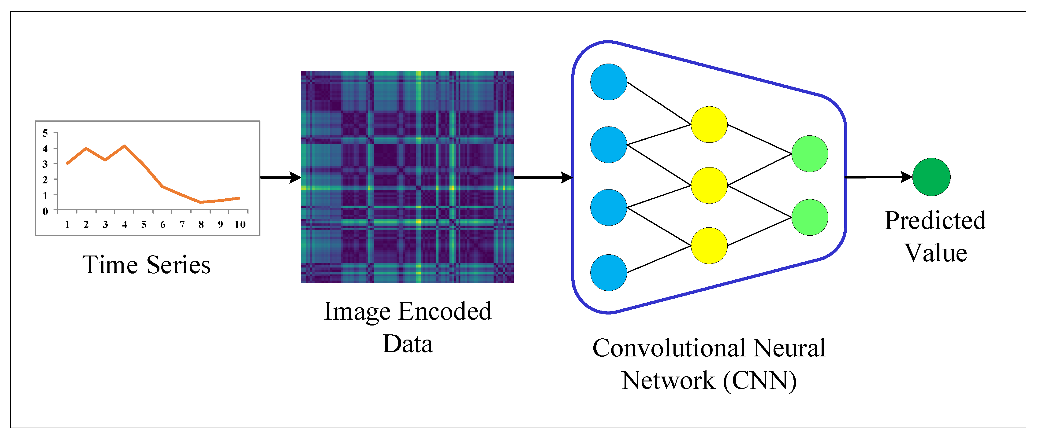
Proposed methodology is discussed in this section. First, the time series forecasting problem is formulated in Section 3.1. Deep learning methods and structures are discussed in Section 3.2. Time series image encoding methods are presented in Section 3.3. Finally, the proposed method based on time series image encoding and deep neural networks is discussed in Section 3.4. The conceptual diagram of the proposed method is depicted in Figure 4.

3.1. Time Series Prediction

Time series can be defined as a sequence of vectors or scalars that depend on time. Time series of vectors can be formulated as the following equation.

$$\{\mathbf{x}\left(t_0\right),\mathbf{x}\left(t_1\right),\mathbf{x}\left(t_2\right),\dots \}$$

(1)

where $t_i$ is the $i^{\mathrm{th}}$ time index. A sample sequence of the load consumption profile is shown in Figure 5. This sequence was extracted from dataset described in Section 4.3.

One of the important tasks in time series is performing forecasting. This task involves predicting the next values of the time series $\mathbf{x}\left(t\right)$. The problem of predicting the next values can be solved using the past values of the time series. From this point of view, the future value can be predicted based on the model that is formulated in (2).

$$\widehat{\mathbf{x}}\left(t_{i+1}\right)=F\left(\mathbf{x}\left(t_i\right),\mathbf{x}\left(t_{i-1}\right),\mathbf{x}\left(t_{i-2}\right),\dots \right)$$

(2)

where F is the prediction function and i is the time index.

3.2. Deep Learning

Deep learning or multiple layer neural networks are a class of machine learning algorithms that are used in regression, clustering, and classification problems. These models are commonly used in audio recognition, image processing [37], machine translation, computer vision [38], medical image segmentation [39,40], and similar applications. In general, deep learning outperforms the traditional machine learning techniques in case the size of data is large, the model is complicated like image classification, and high performance computing is available.

Recently, some of deep learning models including the convolutional neural network (CNN) and recurrent neural network (RNN) [41] have also been applied to the prediction of time series. As the nature of the time series used in forecasting is one-dimensional, one-dimensional CNN (1D CNN) is typically used for regression and forecasting problems. However, the capability of CNN to demonstrate higher performance is beyond applying it to one-dimensional data.

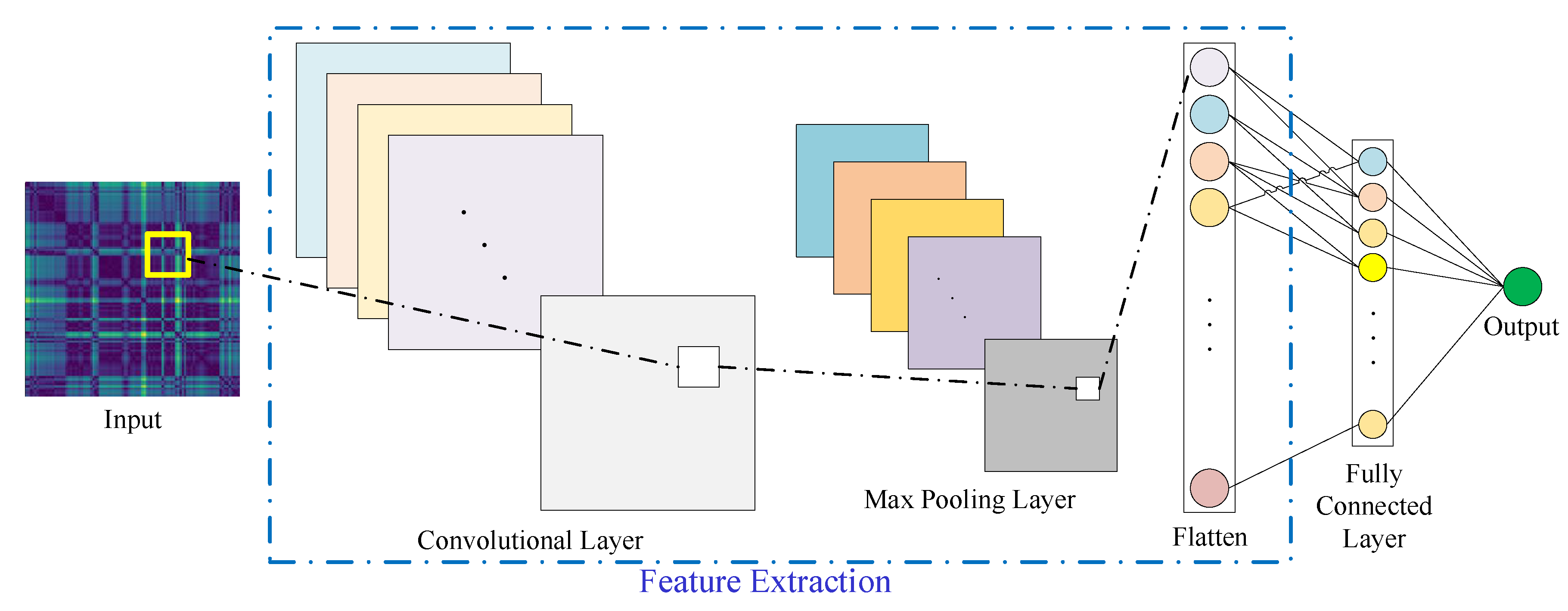
CNN is comprised of convolutional, pooling, and fully connected layers. Convolutional layers can be designed in a 1D or 2D manner. In each convolutional layer, the input data are convolved with a number of filters. Values in the filter are equivalent to weights in neural networks that should be updated during the training procedure based on algorithms like back-propagation. After each convolutional layer, activation functions are applied to add nonlinearity to the system. Pooling layers are used to reduce the spatial dimension in order to control the number of the parameters and overfitting. Finally, fully connected layers map the feature maps to the desired output.

To leverage the capability of CNN, we developed our forecasting method using a two-dimensional convolutional neural network (2D CNN). In this case, the input data to the input layer of the model should be two-dimensional. The CNN model consisted of one convolutional layer and one max pooling layer with 32 filters and a kernel size of 4. After the convolutional layer, we modeled a fully connected layer with 64 nodes. All activation functions were set to be the rectified linear unit (ReLU). Figure 6 shows the structure of the CNN network used.

3.3. Time Series Image Coding

As deep networks have a high capability to recognize and digest images [42], if time series are encoded as images, the performance of the classification and forecasting of them using deep networks would be improved. There are several methods to encode time series into images, including recurrence plots (RP) [43], the Gramian angular field (GAF), and the Markov transition field (MTF) [44]. In the following subsections, these methods are investigated and applied to encode individual household power consumption data as images.

3.3.1. Recurrence Plots

Recurrence plots [45] are generated if the first states in the phase space trajectory of the time series sequence are computed according to the following equation:

$$\mathbf{s}\left(t_i\right)=\left(\mathbf{x}\left(t_i\right),\mathbf{x}\left(t_{i-1}\right)\right)$$

(3)

Then, recurrence plots are formed using the following equation:

$$R(i,j)=dist\left(\mathbf{s}\left(t_i\right),\mathbf{s}\left(t_j\right)\right)$$

(4)

where R is the recurrence plot and $dist$ is the distance function that can be calculated based on the Euclidean distance.

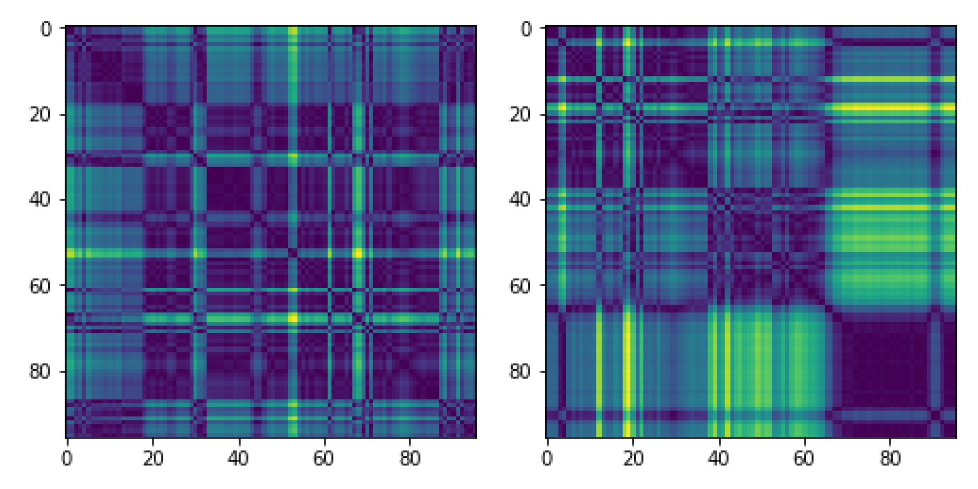
Figure 7 shows the RPs for two different sample times. The dataset used here is described in Section 4.3. As can be seen in this figure, different times ended with different encoded images containing different features.

3.3.2. Gramian Angular Field

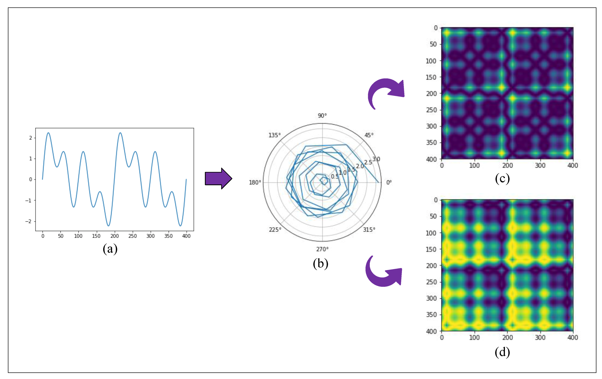
The Gramian angular field is a method of encoding time series into images. This method uses polar mapping to map time series data into a polar plane (see Figure 8b). To generate the Gramian angular field, first, the given time series should be rescaled in the interval $[1,-1]$ following the equation below [46]:

$$\tilde{x}=\frac{(x_i-max\left(x\right))+(x_i-min\left(x\right))}{max\left(x\right)-min\left(x\right)}$$

(5)

Then, the rescaled data are represented in polar coordinates using the following equation:

$${\varphi }_i=arccos\left({\tilde{x}}_i\right)$$

(6)

After transforming the rescaled time series data, the Gramian angular summation field (GASF) and the Gramian angular difference field (GADF) are defined by considering the sum of or difference between each two point pair following the equations below:

$$\mathrm{GASF}(i,j)=cos({\varphi }_i-{\varphi }_j)$$

(7)

$$\mathrm{GADF}(i,j)=sin({\varphi }_i-{\varphi }_j)$$

(8)

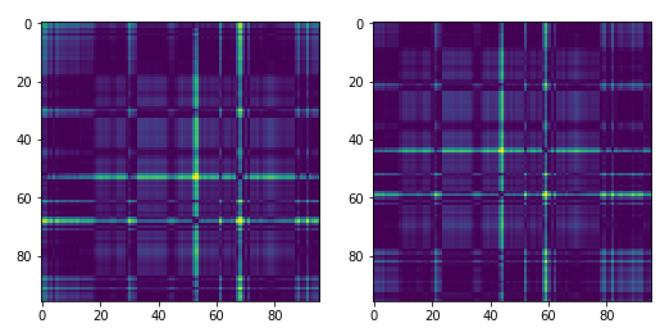
Figure 8c,d shows GASF and GADF for the sample time series in Figure 8a. Figure 9 shows GASFs for two different sample times. The dataset described in Section 4.3 was used here to generate data. As can be seen in this figure, different times ended with different encoded images containing different features.

3.3.3. Markov Transition Field

The Markov transition field is defined as the following matrix [46]:

$$\left[\begin{array}{ccc}{w}_{ij|x_1\in q_i,x_1\in q_j}& \cdots & w_{ij|x_1\in q_i,x_n\in q_j}\\ w_{ij|x_2\in q_i,x_1\in q_j}& \cdots & w_{ij|x_2\in q_i,x_n\in q_j}\\ ⋮& \ddots & ⋮\\ w_{ij|x_n\in q_i,x_1\in q_j}& \cdots & w_{ij|x_n\in q_i,x_n\in q_j}\end{array}\right]$$

(9)

Dividing the data magnitude into Q quantile bins would generate the Q by Q matrix. The quantile bins containing the data at time step i and j are $q_i$ and $q_j$. $w_{ij}$ in the matrix is the transition probability of $q_i\to q_j$. Encoding procedure of Markov transition field is depicted in Figure 10.

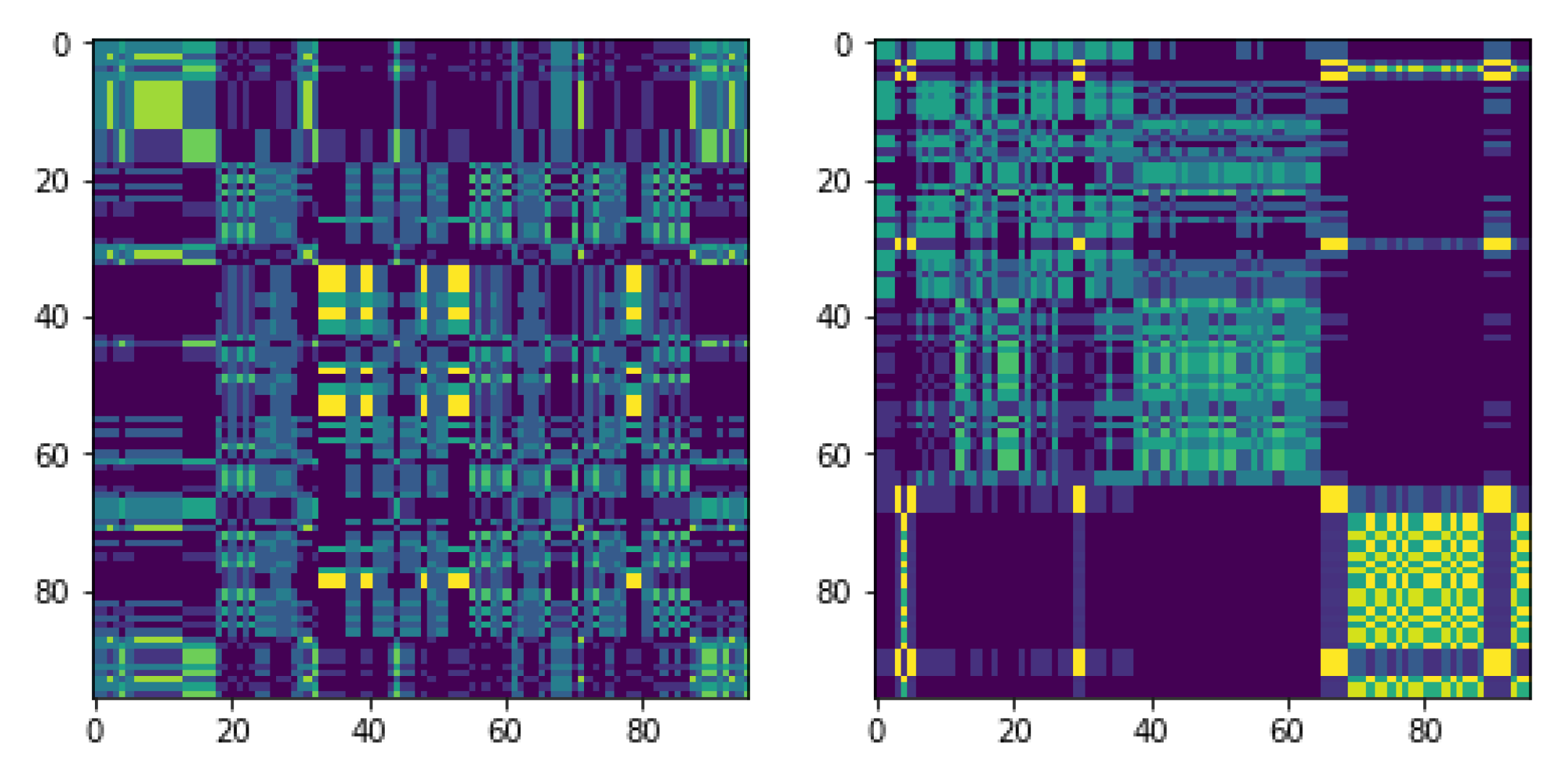
Figure 11 shows the MTFs for two different sample times. The dataset used here is described in Section 4.3. As can be seen in this figures different times ended with different encoded images containing different features.

3.4. Proposed Method

In Figure 4, the block diagram of the proposed method is depicted. At first, time series data are encoded into an image, then the generated image is fed into deep CNN to predict the next value of the time series data. Details of the deep 2D CNN used are illustrated in Figure 6.

CNN network that was used in this study consisted of one 2D convolutional layer, one max pooling layer, and two dense layers. The convolutional layer was comprised of 32 filters with a kernel size of 4. The first fully connected layer consisted of 64 nodes. The last fully connected layer had one node to provide the final estimated value. The rectified linear unit (ReLU) was used as an activation function for both convolutional and dense layers. RMS optimizer was used to compile the model. The maximum number of epochs was set to 100 in the experiments. Eighty percent and 20 percent of all data were used as the training and test sets, respectively.

4. Experiments and Results

In this section, the evaluation criteria are defined in Section 4.1. The datasets used are described in Section 4.2 and Section 4.3. The conducted experiments and comparison results to evaluate the proposed method are discussed in Section 4.4.

4.1. Evaluation Criteria

To evaluate quantitatively, three common criteria were used: mean absolute error (MAE), root mean squared error (RMSE), and mean absolute percentage error (MAPE). These metrics are defined in Equations (10)–(12).

$$\mathrm{MAE}=\frac{{\sum }_{i=1}^N\mid \widehat{\mathbf{y}}\left(t_i\right)-\mathbf{y}\left(t_i\right)\mid }{N}$$

(10)

where $\widehat{\mathbf{y}}$ and $\mathbf{y}$ are the predicted and true values of the test samples, respectively, and Nis the total number of test samples.

$$\mathrm{RMSE}=\sqrt{\frac{{\sum }_{i=1}^N{\left(\widehat{\mathbf{y}}\left(t_i\right)-\mathbf{y}\left(t_i\right)\right)}^2}{N}}$$

(11)

$$\mathrm{MAPE}=\frac{100\%}{N}\sum _{i=1}^N\mid \frac{\widehat{\mathbf{y}}\left(t_i\right)-\mathbf{y}\left(t_i\right)}{\mathbf{y}\left(t_i\right)}\mid$$

(12)

4.2. Boston Housing Dataset

Boston housing price data [47] were used for the comparison of the four different signal to image transformations discussed in Section 3.3. This dataset is available online [48]. Results are summarized in

Table 1. Comparison of different transformations (GASF, GADF, MTF, RP) based on MAE, RMSE, and MAPE.

Methods	MAE	RMSE	MAPE
GASF	1.08	5.95	17.43
GADF	3.35	4.96	14.39
MTF	6.75	8.71	34.89
RP	1.12	3.92	14.15

. Results clearly proved that the recurrence plots could be the best choice in terms of accuracy improvement, so in the next experiment, RPs were used to encode time series into images.

4.3. Load Forecasting Dataset

In this paper, the historic data of a single residential customer from [49] is used to assess the performance of the proposed method comparing to other methods. This dataset contains 2,075,259 samples measured by a smart meter installed at a house near Sceaux (7 km from Paris, France). The samples were periodically retrieved and recorded from December 2006 to November 2010 (47 months).

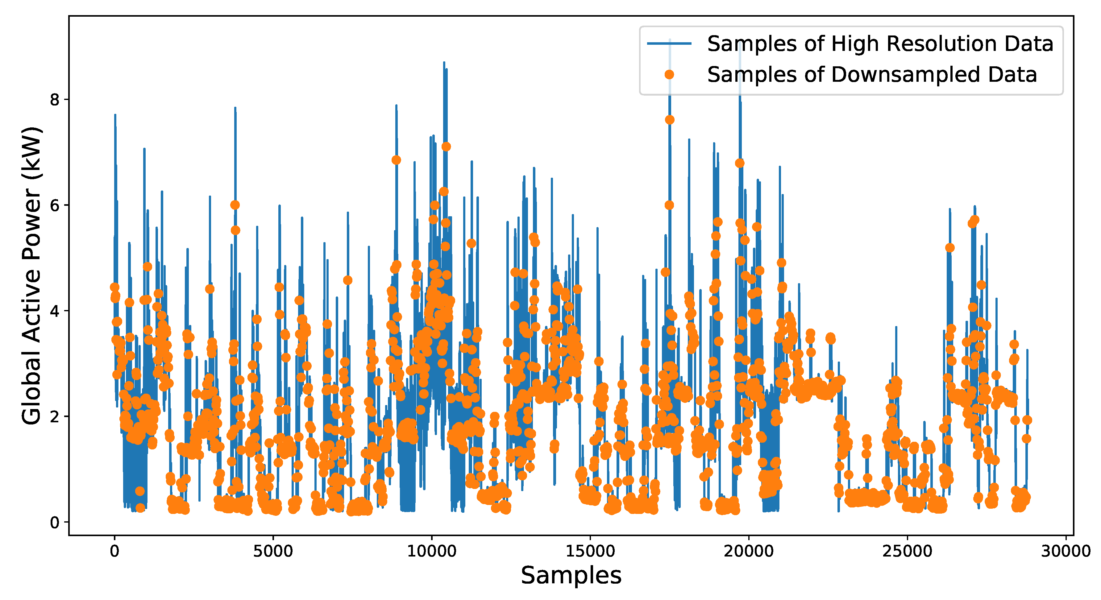
We down-sampled the data to 96 samples per day, for every 15 min. This is because in Advanced Metering Infrastructure (AMI), data are typically collected as measurements from the meters, or pushed as commands to devices every 15 min to ensure a wealth of granular data exchange for demand response service. There were some missing values in this dataset, which we replaced by the average of available measurements at that time section in other years [50]. Down-sampled data in conjunction with original high resolution data are plotted in Figure 12.

4.4. Results

The performance of the proposed method was evaluated in comparison with three different methods: support vector machine (SVM) [8], artificial neural network (ANN) [9], and convolutional neural network (CNN) [10]. The proposed method based on three different image encoding methods was evaluated, and based on the Boston housing dataset results, recurrence plots were used in this experiment.

The proposed algorithm and also the other methods to compare were implemented using Python, Tensorflow, sklearn, and pyts. CNN consisting of one convolutional layer, one pooling layer, and one fully connected layer was used in this study. More details of the proposed method are discussed in Section 3.4.

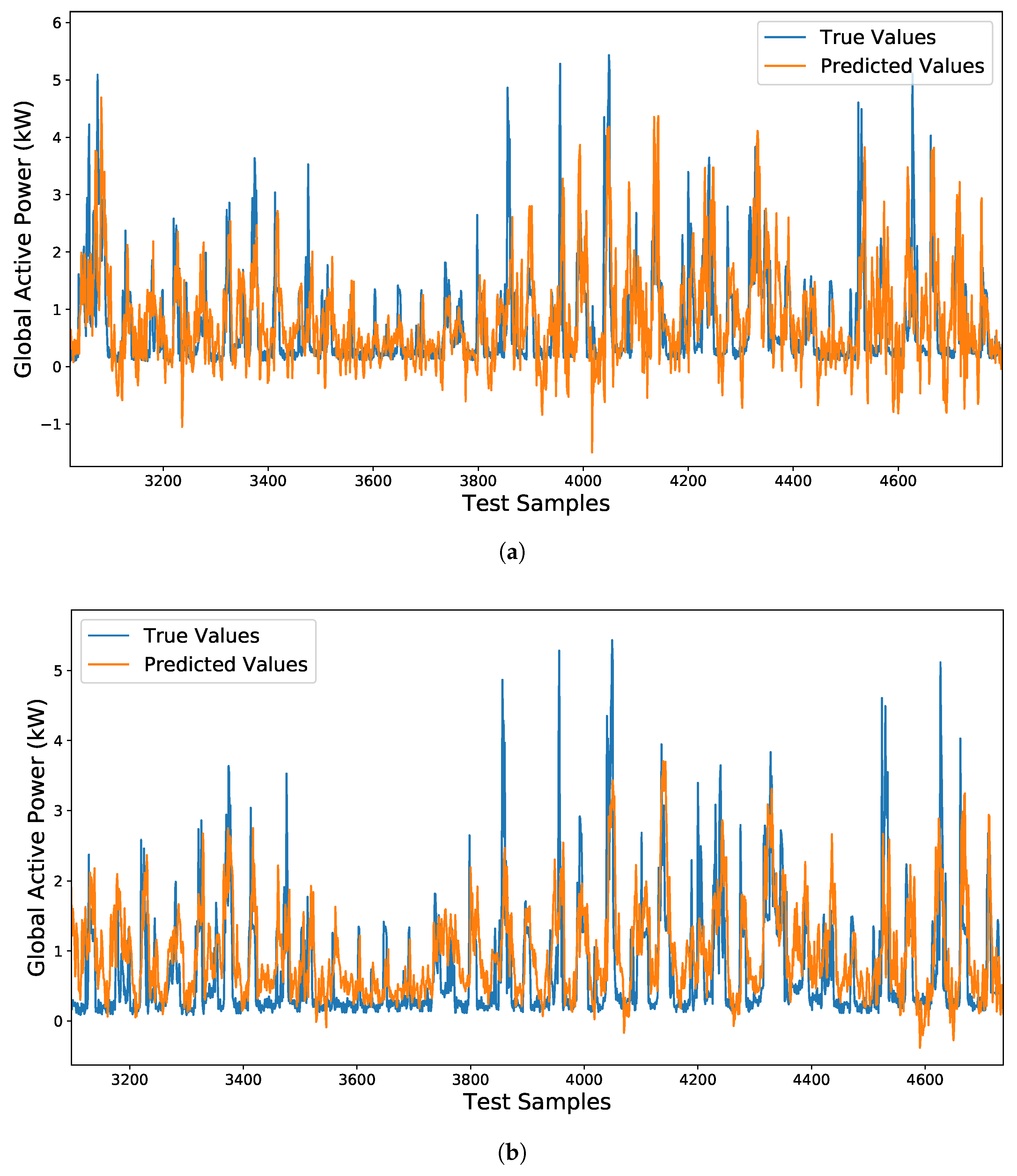
In Figure 13a,b, the predicted and true values of test samples are compared. These figures demonstrate that the 2D method could forecast the next values with a higher accuracy than the 1D CNN.

Table 2. Comparison of different methods based on MAE, RMSE, and MAPE.

Methods	MAE	RMSE	MAPE
SVM	1.12	1.25	25.56
ANN	1.08	1.15	23.25
CNN-1D	0.68	0.92	18.63
CNN-2D-RP	0.59	0.79	12.54

shows the comparison of the proposed method, 1D CNN, ANN, and SVM based on MAE, RMSE, and MAPE. As shown, the proposed method outperformed the compared methods in terms of the defined criteria.

5. Conclusions

In order to apply demand response properly and efficiently, single residential loads should be also predicted. Reviewing the literature, a limited number of methods have been presented for load forecasting at the individual household level. The performance of these methods in terms of accuracy was also quite low compared to their peers in aggregated levels such as building levels or substation levels. The lowest MAPE, reported in the literature, was 12.78% for daily forecast and 23.31% for hourly forecast. Applying CNN was proven to improve the performance, especially for 15 min load forecasting. However, deep networks like CNN showed a high ability to understand images. We proposed a CNN based method that encoded one-dimensional time series into images, firstly. We showed that the RP image encoding technique would result in the lowest MAPE compared to the GASF, GADF, and MTF methods.

Results based on MAE, RMSE, and MAPE criteria showed that our proposed method using RP performed better (MAPE of 12.54%) in comparison with one-dimensional CNN and other classic machine learning methods, namely SVM and ANN. The proposed method outperforms its 1D counterpart by about 20% in terms of RMSE. However, it should be noted that generating image encoded data would increase the computational complexity of the proposed algorithm, which is a limit for real-time applications.

References

1. Basit, A.; Ahmad, T.; Yar Ali, A.; Ullah, K.; Mufti, G.; Hansen, A.D. Flexible Modern Power System: Real-Time Power Balancing through Load and Wind Power. Energies 2019, 12, 1710. [Google Scholar] [CrossRef] [Green Version]
2. Estebsari, A.; Pons, E.; Huang, T.; Bompard, E. Techno-economic impacts of automatic undervoltage load shedding under emergency. Electr. Power Syst. Res. 2016, 131, 168–177. [Google Scholar] [CrossRef] [Green Version]
3. Estebsari, A.; Huang, T.; Pons, E.; Bompard, E. Electricity infrastructure enhancement for the security of supply against coordinated malicious attacks. In Proceedings of the 2016 IEEE 16th International Conference on Environment and Electrical Engineering (EEEIC), Florence, Italy, 7–10 June 2016; pp. 1–6. [Google Scholar] [CrossRef] [Green Version]
4. Wang, Y.; Zhang, N.; Kang, C.; Miao, M.; Shi, R.; Xia, Q. An Efficient Approach to Power System Uncertainty Analysis With High-Dimensional Dependencies. IEEE Trans. Power Syst. 2018, 33, 2984–2994. [Google Scholar] [CrossRef]
5. Zahid, M.; Ahmed, F.; Javaid, N.; Abbasi, R.A.; Zainab Kazmi, H.S.; Javaid, A.; Bilal, M.; Akbar, M.; Ilahi, M. Electricity Price and Load Forecasting using Enhanced Convolutional Neural Network and Enhanced Support Vector Regression in Smart Grids. Electronics 2019, 8, 122. [Google Scholar] [CrossRef] [Green Version]
6. Fallah, S.N.; Ganjkhani, M.; Shamshirband, S.; Chau, K.W. Computational Intelligence on Short-Term Load Forecasting: A Methodological Overview. Energies 2019, 12, 393. [Google Scholar] [CrossRef] [Green Version]
7. Hussain Nengroo, S.; Umair Ali, M.; Zafar, A.; Hussain, S.; Murtaza, T.; Junaid Alvi, M.; Raghavendra, K.; Jee Kim, H. An Optimized Methodology for a Hybrid Photo-Voltaic and Energy Storage System Connected to a Low-Voltage Grid. Electronics 2019, 8, 176. [Google Scholar] [CrossRef] [Green Version]
8. Chen, B.J.; Chang, M.W.; lin, C.J. Load forecasting using support vector Machines: A study on EUNITE competition 2001. IEEE Trans. Power Syst. 2004, 19, 1821–1830. [Google Scholar] [CrossRef] [Green Version]
9. Park, D.C.; El-Sharkawi, M.A.; Marks, R.J.; Atlas, L.E.; Damborg, M.J. Electric load forecasting using an artificial neural network. IEEE Trans. Power Syst. 1991, 6, 442–449. [Google Scholar] [CrossRef] [Green Version]
10. Amarasinghe, K.; Marino, D.L.; Manic, M. Deep neural networks for energy load forecasting. In Proceedings of the 2017 IEEE 26th International Symposium on Industrial Electronics (ISIE), Edinburgh, UK, 19–21 June 2017; pp. 1483–1488. [Google Scholar] [CrossRef]
11. Stevic, M.; Estebsari, A.; Vogel, S.; Pons, E.; Bompard, E.; Masera, M.; Monti, A. Multi-site European framework for real-time co-simulation of power systems. IET Gener. Transm. Distrib. 2017, 11, 4126–4135. [Google Scholar] [CrossRef] [Green Version]
12. Popavath, L.N.; Kaliannan, P. Photovoltaic-STATCOM with Low Voltage Ride through Strategy and Power Quality Enhancement in a Grid Integrated Wind-PV System. Electronics 2018, 7, 51. [Google Scholar] [CrossRef] [Green Version]
13. Sorkin, O.; Farber, E.; Averbukh, M. Selecting Ultracapacitors for Smoothing Voltage Deviations in Local Grids Fed by Transformer with Tap-Changer and Distributed PV Facilities. Electronics 2019, 8, 357. [Google Scholar] [CrossRef] [Green Version]
14. Elrayyah, A.; Bayhan, S. Multi-Channel-Based Microgrid for Reliable Operation and Load Sharing. Energies 2019, 12, 70. [Google Scholar] [CrossRef] [Green Version]
15. Barbierato, L.; Estebsari, A.; Pons, E.; Pau, M.; Salassa, F.; Ghirardi, M.; Patti, E. A Distributed IoT Infrastructure to Test and Deploy Real-Time Demand Response in Smart Grids. IEEE Internet Things J. 2018, 6, 1136–1146. [Google Scholar] [CrossRef]
16. Muratori, M.; Rizzoni, G. Residential Demand Response: Dynamic Energy Management and Time-Varying Electricity Pricing. IEEE Trans. Power Syst. 2016, 31, 1108–1117. [Google Scholar] [CrossRef]
17. Mohsenian-Rad, A.; Leon-Garcia, A. Optimal Residential Load Control With Price Prediction in Real-Time Electricity Pricing Environments. IEEE Trans. Smart Grid 2010, 1, 120–133. [Google Scholar] [CrossRef]
18. Shao, S.; Pipattanasomporn, M.; Rahman, S. Grid Integration of Electric Vehicles and Demand Response With Customer Choice. IEEE Trans. Smart Grid 2012, 3, 543–550. [Google Scholar] [CrossRef]
19. Vivekananthan, C.; Mishra, Y.; Ledwich, G.; Li, F. Demand Response for Residential Appliances via Customer Reward Scheme. IEEE Trans. Smart Grid 2014, 5, 809–820. [Google Scholar] [CrossRef]
20. Khan, A.R.; Mahmood, A.; Safdar, A.; Khan, Z.A.; Khan, N.A. Load forecasting, dynamic pricing and DSM in smart grid: A review. Renew. Sustain. Energy Rev. 2016, 54, 1311–1322. [Google Scholar] [CrossRef]
21. Cai, H.; Shen, S.; Lin, Q.; Li, X.; Xiao, H. Predicting the Energy Consumption of Residential Buildings for Regional Electricity Supply-Side and Demand-Side Management. IEEE Access 2019, 7, 30386–30397. [Google Scholar] [CrossRef]
22. Stephen, B.; Tang, X.; Harvey, P.R.; Galloway, S.; Jennett, K.I. Incorporating Practice Theory in Sub-Profile Models for Short Term Aggregated Residential Load Forecasting. IEEE Trans. Smart Grid 2017, 8, 1591–1598. [Google Scholar] [CrossRef] [Green Version]
23. Ponoćko, J.; Milanović, J.V. Forecasting Demand Flexibility of Aggregated Residential Load Using Smart Meter Data. IEEE Trans. Power Syst. 2018, 33, 5446–5455. [Google Scholar] [CrossRef] [Green Version]
24. Nokar, M.A.; Tashtarian, F.; Moghaddam, M.H.Y. Residential power consumption forecasting in the smart grid using ANFIS system. In Proceedings of the 2017 7th International Conference on Computer and Knowledge Engineering (ICCKE), Mashhad, Iran, 26–27 October 2017; pp. 111–118. [Google Scholar] [CrossRef]
25. Paoletti, S.; Casini, M.; Giannitrapani, A.; Facchini, A.; Garulli, A.; Vicino, A. Load forecasting for active distribution networks. In Proceedings of the 2011 2nd IEEE PES International Conference and Exhibition on Innovative Smart Grid Technologies, Manchester, UK, 5–7 December 2011; pp. 1–6. [Google Scholar] [CrossRef]
26. Xu, L.; Wang, S.; Tang, R. Probabilistic load forecasting for buildings considering weather forecasting uncertainty and uncertain peak load. Appl. Energy 2019, 237, 180–195. [Google Scholar] [CrossRef]
27. Cai, M.; Pipattanasomporn, M.; Rahman, S. Day-ahead building-level load forecasts using deep learning vs. traditional time-series techniques. Appl. Energy 2019, 236, 1078–1088. [Google Scholar] [CrossRef]
28. Shaad, M.; Momeni, A.; Diduch, C.P.; Kaye, M.E.; Chang, L. Forecasting the power consumption of a single domestic electric water heater for a direct load control program. In Proceedings of the 2015 IEEE 28th Canadian Conference on Electrical and Computer Engineering (CCECE), Halifax, NS, Canada, 3–6 May 2015; pp. 1550–1555. [Google Scholar] [CrossRef]
29. Kouzelis, K.; Tan, Z.H.; Bak-Jensen, B.; Pillai, J.R.; Ritchie, E. Estimation of Residential Heat Pump Consumption for Flexibility Market Applications. IEEE Trans. Smart Grid 2015, 6, 1852–1864. [Google Scholar] [CrossRef]
30. Hu, X.; Ferrera, E.; Tomasi, R.; Pastrone, C. Short-term load forecasting with Radial Basis Functions and Singular Spectrum Analysis for residential Electric Vehicles recharging control. In Proceedings of the 2015 IEEE 15th International Conference on Environment and Electrical Engineering (EEEIC), Rome, Italy, 10–13 June 2015; pp. 1783–1788. [Google Scholar] [CrossRef]
31. Wang, J.; Li, G.; Chen, H.; Liu, J.; Guo, Y.; Sun, S.; Hu, Y. Energy consumption prediction for water-source heat pump system using pattern recognition based algorithms. Appl. Therm. Eng. 2018, 136, 755–766. [Google Scholar] [CrossRef]
32. Salerno, V.M.; Rabbeni, G. An Extreme Learning Machine Approach to Effective Energy Disaggregation. Electronics 2018, 7, 235. [Google Scholar] [CrossRef] [Green Version]
33. Sevlian, R.A.; Rajagopal, R. A model for the effect of aggregation on short term load forecasting. In Proceedings of the 2014 IEEE PES General Meeting | Conference Exposition, National Harbor, MD, USA, 27–31 July 2014; pp. 1–5. [Google Scholar] [CrossRef]
34. Kong, W.; Dong, Z.Y.; Luo, F.; Meng, K.; Zhang, W.; Wang, F.; Zhao, X. Effect of automatic hyperparameter tuning for residential load forecasting via deep learning. In Proceedings of the 2017 Australasian Universities Power Engineering Conference (AUPEC), Melbourne, Australia, 19–22 November 2017; pp. 1–6. [Google Scholar] [CrossRef]
35. Kong, W.; Dong, Z.Y.; Jia, Y.; Hill, D.J.; Xu, Y.; Zhang, Y. Short-Term Residential Load Forecasting based on LSTM Recurrent Neural Network. IEEE Trans. Smart Grid 2017, 10, 841–851. [Google Scholar] [CrossRef]
36. Zhang, X.M.; Grolinger, K.; Capretz, M.A.M.; Seewald, L. Forecasting Residential Energy Consumption: Single Household Perspective. In Proceedings of the 2018 17th IEEE International Conference on Machine Learning and Applications (ICMLA), Orlando, FL, USA, 17–20 December 2018; pp. 110–117. [Google Scholar] [CrossRef]
37. Wang, S.H.; Sun, J.; Phillips, P.; Zhao, G.; Zhang, Y.D. Polarimetric synthetic aperture radar image segmentation by convolutional neural network using graphical processing units. J. Real-Time Image Process. 2018, 15, 631–642. [Google Scholar] [CrossRef]
38. Zhang, Y.D.; Dong, Z.; Chen, X.; Jia, W.; Du, S.; Muhammad, K.; Wang, S.H. Image based fruit category classification by 13-layer deep convolutional neural network and data augmentation. Multimedia Tools Appl. 2019, 78. [Google Scholar] [CrossRef]
39. Jaworek-Korjakowska, J. A Deep Learning Approach to Vascular Structure Segmentation in Dermoscopy Colour Images. BioMed Res. Int. 2018, 2018, 5049390. [Google Scholar] [CrossRef] [Green Version]
40. Jaworek-Korjakowska, J. Acral melanocytic lesion segmentation with a convolution neural network (U-Net). In Medical Imaging 2019: Computer-Aided Diagnosis; International Society for Optics and Photonics: Bellingham, WA, USA, 2019; Volume 10950, p. 109504B. [Google Scholar]
41. LeCun, Y.; Bengio, Y.; Hinton, G. Deep learning. Nature 2015, 521, 436. [Google Scholar] [CrossRef] [PubMed]
42. Ma, X.; Dai, Z.; He, Z.; Ma, J.; Wang, Y.; Wang, Y. Learning traffic as images: A deep convolutional neural network for large-scale transportation network speed prediction. Sensors 2017, 17, 818. [Google Scholar] [CrossRef] [PubMed] [Green Version]
43. Rajabi, R.; Estebsari, A. Deep Learning Based Forecasting of Individual Residential Loads Using Recurrence Plots. In Proceedings of the 2019 IEEE Milan PowerTech, Milan, Italy, 23–27 June 2019; pp. 1–5. [Google Scholar] [CrossRef]
44. Wang, Z.; Oates, T. Encoding time series as images for visual inspection and classification using tiled convolutional neural networks. In Proceedings of the Workshops at the Twenty-Ninth AAAI Conference on Artificial Intelligence, Austin, TX, USA, 25–30 January 2015; Volume 1. [Google Scholar]
45. Hatami, N.; Gavet, Y.; Debayle, J. Classification of time-series images using deep convolutional neural networks. In Tenth International Conference on Machine Vision (ICMV 2017); International Society for Optics and Photonics: Bellingham, WA, USA, 2018; Volume 10696, p. 106960Y. [Google Scholar]
46. Wang, Z.; Oates, T. Imaging time-series to improve classification and imputation. In Proceedings of the Twenty-Fourth International Joint Conference on Artificial Intelligence, Buenos Aires, Argentina, 25–31 July 2015. [Google Scholar]
47. Harrison, D.; Rubinfeld, D.L. Hedonic housing prices and the demand for clean air. J. Environ. Econ. Manag. 1978, 5, 81–102. [Google Scholar] [CrossRef] [Green Version]
48. Harrison, D.; Rubinfeld, D. The Boston House-Price Data. 1978. Data Retrieved from StatLib—Datasets Archive. Available online: http://lib.stat.cmu.edu/datasets/boston (accessed on 24 August 2019).
49. Bache, K.; Lichman, M. Individual Household Electric Power Consumption Data Set. 2012. Data Retrieved from UCI Machine Learning Repository. Available online: https://archive.ics.uci.edu/ml/datasets.html (accessed on 21 August 2019).
50. Mocanu, E.; Nguyen, P.H.; Gibescu, M.; Kling, W.L. Deep learning for estimating building energy consumption. Sustain. Energy Grids Netw. 2016, 6, 91–99. [Google Scholar] [CrossRef]
Figure 1. Different types of load forecasting.
Electronics 09 00068 g001
Figure 2. An example of the application of single residential load forecasting with high accuracy.
Electronics 09 00068 g002
Figure 3. Different types of models used for load forecasting.
Electronics 09 00068 g003
Figure 4. Conceptual block diagram of the proposed structure for individual household power consumption prediction using image encoding techniques and CNN.
Electronics 09 00068 g004
Figure 5. Sample individual residential load profile.
Electronics 09 00068 g005
Figure 6. CNN’s structure.
Electronics 09 00068 g006
Figure 7. Sample recurrence plot of 96 points’ load profile time series calculated at two different time steps.
Electronics 09 00068 g007
Figure 8. Gramian angular field encoding procedure: (a) time series data, (b) polar mapping, (c) Gramian angular summation field (GASF), and (d) Gramian angular difference field (GADF).
Electronics 09 00068 g008
Figure 9. Sample Gramian angular field of 96 points’ load profile time series calculated at two different time steps.
Electronics 09 00068 g009
Figure 10. Markov transition field encoding procedure: (a) time series data, (b) Markov transition matrix, and (c) Markov transition field.
Electronics 09 00068 g010
Figure 11. Sample Markov transition field of 96 points’ load profile time series calculated at two different time steps.
Electronics 09 00068 g011
Figure 12. High resolution and downsampled data by averaging every 15 min.
Electronics 09 00068 g012
Figure 13. Single household power consumption prediction results using (a) CNN-1D and (b) CNN-2D-RP.
Electronics 09 00068 g013