Abstract
In Korea, data on pavement conditions, such as cracks, rutting depth, and the international roughness index, are obtained using automatic pavement condition investigation equipment, such as ARAN and KRISS, for the same sections of national highways annually to manage their pavement conditions. This study predicts the deterioration of road pavement by using monitoring data from the Korean National Highway Pavement Management System and a recurrent neural network algorithm. The constructed algorithm predicts the pavement condition index for each section of the road network for one year by learning from the time series data for the preceding 10 years. Because pavement type, traffic load, and environmental characteristics differed by section, the sequence lengths (SQL) necessary to optimize each section were also different. The results of minimizing the root-mean-square error, according to the SQL by section and pavement condition index, showed that the error was reduced by 58.3–68.2% with a SQL value of 1, while pavement deterioration in each section could be predicted with a high coefficient of determination of 0.71–0.87. The accurate prediction of maintenance timing for pavement in this study will help optimize the life cycle of road pavement by increasing its life expectancy and reducing its maintenance budget.
1. Introduction
With the start of the fourth industrial revolution, technological innovation is in progress to apply information and communication technology, Internet of things (IoT) sensors, big data, and artificial intelligence to realistic tasks. Artificial intelligence technology can be applied to almost all areas of society beyond the traditional IoT industry, but few large leading companies can effectively respond to this high degree of diversity. Therefore, the sustainable development of artificial intelligence technology must involve the government, universities, and public research institutes to achieve open innovation [1].
Advanced countries, such as the USA and Japan, are introducing these new technologies at a national level to increase the efficiency of road pavement maintenance and management [2]. In addition, with research on and development of the property management system using artificial intelligence and big data, it is expected that public infrastructure can be maintained efficiently. Advanced countries are conducting research on and development of pavement management systems for various reasons, such as serviceability, life cycle cost analysis, and pavement design. In particular, in addition to the existing statistical methodologies, research utilizing artificial intelligence has been conducted in various fields, such as pavement performance and distress prediction, pavement management systems and maintenance strategy, structure evaluation of pavement systems, and image recognition to detect pavement distress. Previous studies have shown that artificial intelligence can be widely applied to solve various problems, including the nonlinear problems of pavement engineering [2]. In addition, deep learning and machine learning techniques are being used in various fields for open innovation [3,4,5,6].
In Korea, social infrastructure built intensively in the high growth period of the 1980s is aging; in the case of road pavements, it is expected that 85% of all roads will exceed 20 years of service life in the next 10 years. To prevent the aging of such paved roads, a pavement management system (PMS) is aimed at the systematic maintenance and management of road pavement. A PMS is a tool that systematically manages all phases of road pavement, ranging from basic planning, design, construction, maintenance, and evaluation of road pavement to maintaining the best possible pavement condition with minimal cost. Because a PMS is based on the lifecycle cost analysis of road pavement, it is necessary to reliably analyze the costs incurred in the initial construction phase, as well as the costs incurred at the time of disposal. Therefore, to develop a system for efficient maintenance of paved road, it is very important to develop a model for predicting pavement distress. A variety of studies have been conducted to develop models for predicting pavement distress: Statistical methodologies, including regression, Markov chains, neural networks (NNs), and recurrent neural networks (RNNs), have been used in these studies [7,8,9,10].
The most critical difference between a statistical model and a deep learning model is that the statistical model requires a hypothesis for the data. For example, in a linear regression model, the hypothesis is an assumption that the objective variable can be explained by a linear combination of explanatory variables, while the Markov chain model assumes that the current condition at discrete times is changed by a transition probability that relies only on the condition at the previous time. When the data satisfy such a simplified assumption, the expressive power of the model is greatly restricted, so the analysis of the parameters becomes simple. However, when the assumption about the data is inappropriate, the accuracy of the prediction becomes poor and the interpretation of the parameters becomes difficult. The relationship between the explanatory variables and the objective variable can be observed clearly in controlled conditions, such as in the laboratory. However, in the case of data measured in the field, there are various factors that can be measured but cannot be related to the state of the road pavement, such as environmental conditions and differences in construction quality. Therefore, there is a high probability of large errors between the explanatory variable and the objective variable, and the relationship may be complicated with a nonlinear shape. In these cases, it is difficult to analyze the relationship between variables using conventional statistical models. In contrast, a deep learning model is a highly expressive model that can approximate all nonlinear functions. For example, road pavement condition can be predicted with high accuracy by a RNN model that predicts the distress of a section by finding the distress characteristics per unit interval, including all maintenance histories generated in the relevant interval, or by considering interaction between all explanatory variables and their nonlinear changes. Therefore, a deep learning model considers the relationship between variables that are not included in the existing statistical models. Deep learning could perform excellently in analyzing data obtained from the site that embodies nonlinear and complex relationships.
Therefore, this study aims to develop a road pavement deterioration model using a RNN algorithm, based on the road pavement monitoring (RPM) data from the Korean National Highway Pavement Management System (NHPMS). In particular, environmental variables that were not considered in previous research, such as annual average temperature and annual total precipitation, were considered during model development. First, the literature regarding road pavement deterioration models using deep learning and explanatory variables is reviewed, and then the characteristics of the monitoring data are analyzed. An empirical analysis is then conducted to develop a road pavement deterioration prediction model using the RNN model. Finally, the results of this study are summarized, and conclusions are drawn by verifying the applicability of the RNN algorithm in predicting road pavement condition.
2. Literature Review
It is essential to predict the deterioration condition of the pavement accurately to establish an efficient property management system. Deterioration of the road pavement progresses relatively slowly but continuously and is caused by various environmental factors, such as pavement design, materials, traffic loads, annual average temperature, and annual total precipitation [11,12]. In most studies that have attempted to predict road pavement deterioration, the deterioration speeds have been estimated from the difference between the past and present amounts of deterioration, based on visual inspection data [13]. Shin [14] proposed a semi-parametric stochastic duration model to predict crack deterioration in asphalt pavement. Loizos and Karlaftis [15] also developed a pavement surface distress prediction model based on the probabilistic duration principle. However, existing statistical deterioration models are at a preliminary stage and, if multiple variables are estimated, problems, such as convergence of maximum likelihood estimation (MLE), still exist [16,17]. To solve such problems, some researchers have proposed using a Bayesian estimation method. This has been found to solve problems concerning a small sample quantity and convergence of the estimation function [18,19,20].
In addition to statistical analysis methods, studies using the deep learning methodology have been widely conducted. These can be broadly classified into studies using NN algorithms and those using RNN algorithms. Attoh-Okine [21] used a back-propagation type of NN to develop a deterioration model for the rutting depth index of the road pavement. He trained the NN algorithm with the explanatory variables, such as road structure deformation, traffic loads, crack rate, and rutting depth in the previous year, and surface distress, such as patching. It was found that the prediction performance of the NN algorithm was greatly enhanced when factors, such as road pavement life and environments, were additionally considered. Attoh-Okine [22] also analyzed the road pavement condition using a back-propagation NN to develop a deterioration model for the international roughness index (IRI) of the road pavement. Various input variables and a NN algorithm were also utilized to predict cracking of the road pavement, rutting depth, IRI, the condition rating index (CRI), visual condition index (VCI), and the present serviceability index (PSI) [23,24,25,26,27,28,29]. In addition, it was found that the prediction performance when using the NN algorithm was higher than that achieved using the conventional statistical analysis [30,31].
However, Attoh-Okine [21] pointed out that prediction performance deteriorated if prediction was performed for new data, instead of the data used for learning. This was because of the problem that commonly occurs with NN learning: The algorithm was overfitted to the learning data. To solve the problem of such NN algorithms, various methods have been proposed. Hinton et al. [32] proposed a method of learning a deep belief network after pre-training the data, using the limited Boltzmann machine. However, recently, the dropout normalization technique, which can solve overfitting problems by randomly removing connections between some neurons in the existing deep belief network during the learning process, is often used [33,34]. In a study to predict the service life of a paved road, Choi and Do [31] reported that prediction performance was enhanced, using a NN algorithm, when overfitting was resolved.
In addition, there have been several studies that utilized a RNN algorithm, which is suitable for analyzing time series data. Tabatabaee et al. [35] utilized the support vector machine (SVM) and RNN model to develop a prediction model for the PSI. First, they used the SVM to classify the sections with structural similarities. Second, the RNN model was used to predict the PSI in the following year from the other independent variables, together with the classification results obtained during the first stage. The case study used a dataset from the Ministry of Transportation, Minnesota, USA (MnRoad). This revealed that the second-stage model (which used both the SVM and RNN together) was superior, in terms of prediction performance and error, to the first-stage model (which used only the RNN). Okuda et al. [36] utilized the RNN model to develop a prediction model for rutting depth. When the time series data for road deterioration accumulated for 20 years were used, it was found that the best prediction performance was achieved when the RNN model was used.
Therefore, in this study, the analysis was carried out with the RNN algorithm, not the NN algorithm, to correctly handle the time series data in the RPM dataset. In addition, the aim was to establish a model with an optimum performance for each road pavement section by conducting a sensitivity analysis by sequence length, which is a core element of the RNN algorithm; this contrasts with previous research that has utilized the RNN algorithm, which did not consider sequence length.
3. Characteristics of Data
3.1. Characteristics of Road Pavement Monitoring Data
In this study, the data in the RPM dataset provided by the Korean NHPMS were used to predict the pavement condition index of the individual monitoring sections, whose locations are shown in Figure 1.
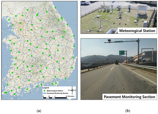
Figure 1.
Pavement monitoring sections and meteorological stations: (a) location, (b) field image.
The RPM dataset contained data for the 11 years from 2007 to 2017, inclusive. RPM data represent the overall pavement conditions of the general national highways. Data are collected annually by pavement condition inspection equipment, such as ARAN and KRISS, for a road span of 2300 km, which is about 20% of the total extent of the national highways. ARAN and KRISS are equipment that can automatically measure road pavement conditions while driving. The main functions include detection of cracks, rutting depth, and IRI, as well as video recording of the pavement section. Crack detection is performed by acquiring a pavement image with an actual crack resolution of less than 1 mm by using a high-resolution line scan camera installed at the rear of the vehicle. The rutting depth is measured using ultrasonic waves, and the IRI can be quantified by attaching a high-precision high-speed radar with a precision of 0.1 mm or less to both wheel segments, facing in the same direction as the vehicle′s driving trajectory. Each section has a length of 1 km, and the same section is investigated every year.
The data contained information such as section length, location, administration office, pavement condition data (crack, rutting depth, and IRI), annual average daily traffic (AADT), equivalent single axle loads (ESAL), and maintenance timing. Maintenance is performed individually for each section, maintenance timings vary depending on the road pavement conditions of each section, and maintenance is performed every 8 to 12 years on average.
The RPM data are summarized in Table 1. The number of sections inspected in each inspection year ranged from 2308 to 2445 and was different each year. The reason for the difference in sections was that inspection could not be conducted, for reasons such as maintenance and repair, construction of the respective sections, or changes in the locations of the monitoring sections. Because the purpose of this study was to predict the pavement condition of the individual monitoring sections characterized by time series data, the sections with pavement condition data for all 11 consecutive years were selected for analysis. The number of sections for which RPM data was used in the final analysis was 1880.

Table 1.
Specification of road pavement monitoring (RPM) dataset.
In general, the status value of the road pavement condition was reset to 0 when maintenance work was performed. The pavement condition deteriorated as time elapsed, and the status value tended to increase. In addition, according to each pavement condition index, the road was damaged by composite factors, which occurred independently of each other. Table 1 shows the average pavement condition for the 1880 sections. Until the year 2012, the rutting depth was decreasing, whereas the crack and IRI were increasing. This implies that the maintenance work until 2012 focused on sections where plastic strain had occurred. After that year, the road pavement condition worsened regardless of the road pavement status index. The overall road pavement condition has been improving since 2016.
The standard deviations for each pavement condition index for each year is shown in Table 1. Compared with other indices, the distribution of crack rate is very different from the year 2013. The standard deviations of crack rate between 2007 and 2012 were 5.3–6.5, but these significantly increased to 8.9–11.4 after 2013. This is because of changes to the vendors of the equipment for inspecting road pavement condition and the method of calculating crack rates, which were manually calculated, in contrast to rutting depth and IRI, which were measured automatically by the equipment. Therefore, in this study, a change of inspection equipment was set as a dummy variable and applied to the deep learning analysis from 2013.
3.2. Selection of Explanatory Variables and Generation of Analysis Data
The Specification of Explanatory variables are summarized in Table 2. The independent variables that were used in the analysis were broadly categorized into average daily traffic variables, environmental variables, and dummy variables. First, for the average daily traffic variables, data were obtained by dividing the AADT and ESAL data in each section (which could be obtained from the RPM data) by the number of lanes in the section.
Table 2.
Specification of explanatory variables.
For the environmental variables for each section, data from the annual weather reports provided by the Korea Meteorological Administration (KMA) were used. Among the 81 locations for which data could be obtained, the data for 74 locations (excluding the locations in the islands) were used. The data for snowfall amounts, which were anticipated to have affected road pavement deterioration, were excluded because data were missing from some of the weather stations. Therefore, annual average temperature, annual maximum average temperature, annual minimum average temperature, and annual total precipitation were used for the analysis. The standard deviation of weather data was shown to be somewhat low, implying that the weather differences between the regions were relatively small at first. Moreover, the average of the annual data between the meteorological stations was utilized, rather than the monthly data. To match the environmental variables that are provided by the KMA to the RPM data, the KMA location nearest to each section was selected by utilizing the ArcGIS software.
Deicing agents mainly use calcium chloride or sodium chloride, and excessive use may affect road pavement damage. Therefore, the amount of desiccant use was considered as an explanatory variable in this study. For the amount of deicing agent used for the general national highway, the data in the Road Deicing System of the Ministry of Land, Infrastructure, and Transport were used. The deicing agent data are provided as a total amount by each National Land Administration Office, not by the general national highway route or by section. The national highway is divided into 18 National Land Administration Offices, so the road pavement monitoring section can be divided into 18 areas. Therefore, data on the amount of deicing agent used for each local land management office were matched to the monitoring section managed by the National Land Administration Office and utilized for analysis.
The analysis data for model development were set with the dependent variables of rutting depth, crack rate, and IRI, which were the pavement condition indices of each section. The independent variables were AADT, ESAL, annual average temperature, annual total precipitation, annual maximum average temperature, annual minimum average temperature, amount of deicing agent used, and pavement condition inspection equipment (which was set as a dummy variable).
The coefficients of determination by section, between each independent variable and each dependent variable (pavement condition index), excluding the dummy variables, are shown in Table 3. The coefficient of determination was very low, with an average of 0.10–0.26 over all pavement condition indices, which indicates that each independent variable has relatively little effect on the road pavement deterioration.
Table 3.
Coefficients of determination (R2 values) between variables.
The crack rate was found to be affected most by AADT, deicing, and ESAL, whereas the rutting depth was found to be affected most by the annual average temperature, annual maximum temperature, and IRI by the AADT and deicing index. This confirms that the independent variables that affect each pavement condition index were different from each other, despite the overall low coefficient of determination. Furthermore, each variable had a high maximum coefficient of determination, 0.64–0.97, which confirms that there were sections heavily influenced by each independent variable.
The results show that the effect of the independent variables on the deterioration of the road pavement was relatively small, from a statistical perspective. This might be because the data for AADT and ESAL were obtained from the inspection locations near the RPM section, not from the RPM section itself, and the weather data were sometimes obtained from distant weather stations. Despite the low statistical relationship, the RNN algorithm was used with these independent variables to predict the road pavement condition indices in this study.
4. Methodology
Deep learning refers to the use of algorithms in which hidden layers are added to the existing neural network structure. The software that helps analysis and development to be conducted easily using a deep learning algorithm is known as a deep learning framework and is mostly distributed in the form of open-source software. Representative deep learning frameworks include Theano, TensorFlow, Torch, Caffe, MXnet, CNTK, and Keras, and it is very important to select a framework that is appropriate for the analysis purpose and data type. Among these software products, TensorFlow has a structure that focuses on the structure of the deep learning from the researcher’s perspective, not on hardware elements, so it has the merit of improving productivity [36]. Therefore, TensorFlow 1.5 was the deep learning open-source framework selected for this study.
A RNN has the added ability to handle time series data, unlike a general neural network, because of its ability to memorize the previous information in the hidden layer. Because RNNs have an added recurrent time series structure, the information can be sustained internally, learning proceeds by memorizing past data in the hidden area. Therefore, it is a suitable model for time series data.
Figure 2 shows the profile of the recurrent structure of the RNN. The RNN repeatedly receives the input data and previous data together and processes them. Therefore, it is possible for it to learn the effect of the past data on the subsequent data. With these characteristics, RNNs can be used to predict time series data, such as stock prices, whose input data take the form of a time sequence.
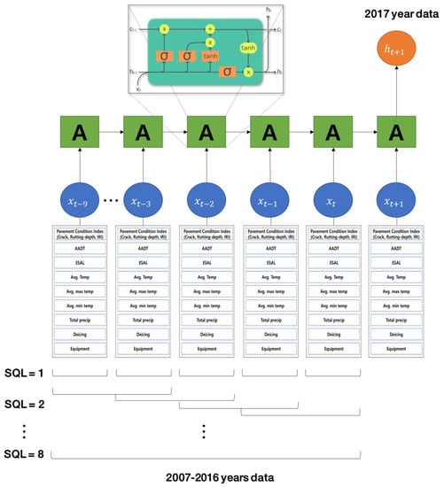
Figure 2.
Structure of the recurrent neural network (RNN).
Long short-term memory (LSTM) solves the vanishing gradient problem of the RNN and makes it effective in capturing long-term dependencies. Therefore, it is effective in learning issues associated with various time series data and can be extended. It is already being utilized in voice recognition, language modeling, translation, and other fields, in combination with other neural networks.
The structure of LSTM is shown in Figure 2. It is composed of a memory movement cell that can maintain a state over time and three nonlinear gates that control data flow in and out of the cell. That is, LSTM introduces a concept called a cell () to update the status () at a specific time and decide whether information inside should be updated by using the status from the input until now. In addition, there are several gate types: the input gate (), forget gate (), and output gate (), which control the data flow of the cell. The forget gate () can be determined by Equation (1).
The output of the previous cell () and the current input () are applied in the sigmoid function active layer to obtain a value in the range [0,1]. This value is multiplied by the current state and the elements, and the cell chooses whether to retain or remove this information during the process.
where represents the activation function, is the weight of the forget gate, and is the bias. In the input gate it is decided which information shall be stored in the cell, as shown in Equation (2). This process is broadly categorized into two stages: (1) decide what to update by using the sigmoid function, and (2) create a candidate cell () which is used during a new cell status update by using the hyperbolic tangent (tanh) function, through Equation (3).
where are the weights of the input gate and candidate cell, respectively, and represent the biases of the input gate and candidate cell, respectively. After this, the cell status () (in the past) and the candidate cell status () are combined, as shown in Equation (4), and the current cell status () is updated.
Finally, the output gate decides which part of the cell status should be the output by using the sigmoid function, as in Equation (5). The cell status is multiplied by the activated cell status () by using the hyperbolic tangent function, as shown in Equation (6), to update the status () at a specific time.
where is the weight of the output gate and is the bias.
LSTM calculates the final output values through the hidden variables, with the method similar to that of a standard RNN. However, LSTM adjusts the information flow by appropriately using the gates during the variable calculation process of the hidden layer. As a result, the RNN using LSTM cells handles gradient loss without any problem, even for data with long process sequences, such as time series data of stock prices.
5. Results and Discussion
5.1. Optimization of Recurrent Neural Network
In general, the hyperparameters of the RNN algorithm comprise the learning rate, number of epochs, and sequence length (SQL). An optimal model is constructed by heuristic methods, such as a trial and error method. As mentioned in Section 1, in this study, a prediction model was intended to be developed for each pavement condition by the RPM section, not by the individual performance prediction model for the pavement condition indices (crack rate, rutting depth, and IRI).
The data structures are summarized in Table 4. A RNN algorithm was constructed to predict the pavement condition indices for the year 2017 by utilizing the time series data for 10 years from 2007 to 2016 as learning and test data. To prepare the learning model, 70% of the data were used, and the remaining 30% were used for testing data. This algorithm learned (or tests) the time series data for 10 years, and the SQL usable for optimizing the algorithm was limited to a maximum of 8. The reason is that, if SQL was 9, the datasets for 2007–2015 were required to predict the pavement condition in the year 2016. In this case, with only the datasets for 2007–2015, the minimum dataset criteria (at least 2 datasets were required for dividing the train and test data sets) could not be satisfied.
Table 4.
Data structures of sequence lengths (SQL) and number of data sets.
The following are some examples of the implementation process of the LSTM model. SQL 1 indicates that the pavement condition is predicted based on the t year pavement condition indicators and explanatory variables, while only considering the description variables of t + 1 (same as the NN algorithm). Moreover, SQL 3 refers to the use of data for three years (t − 2 to t years) to predict the pavement condition index for t + 1 years.
The Parameters of the RNN algorithm are summarized in Table 5. A total of 1880 sections were used for analysis. The number of epochs (repetitions of learning) needs to be decided: Learning should be stopped when the best prediction model has been constructed. It is important to stop learning at an early stage because computing resources are limited and learning time is restricted. The optimal number of epochs can be determined by plotting the number of epochs against the loss function result. In this study, experiments showed that the best loss function could be obtained when the number of epochs was between 400 and 500, and the loss value was almost unchanged after 500 rounds.
Table 5.
Parameters of the RNN algorithm.
Therefore, to establish a model with an optimal performance for each section, the learning rate was maintained as 0.001 and the number of epochs was set to 500 consistently in this study.
In addition, by varying the SQL between 1 and 8, the value that minimized the root-mean-square error (RMSE) was judged to be the optimized value of SQL for each section.
First, as shown in Figure 3a, the RMSE and the coefficient of determination (R2) in all of the sections, for each value of SQL, were examined. As the SQL increased, the RMSE decreased and the R2 values increased. When SQL was 8, the RMSE of the crack rate decreased by 19%, the rutting depth RMSE decreased by 19.4%, and the IRI RMSE decreased by 28.2%, as compared with the values when SQL was 1. The R2 for the crack rate increased by 221.8%, the rutting depth by 56.6%, and the IRI by 57.9%. This might be because the time series data required for the prediction of the pavement condition indices for the year 2017 were increased as the SQLs increased. Figure 3b shows the number of sections for which RMSE was minimized by each value of SQL. The RMSE was minimized when SQL was 8 for a large number of sections and for all pavement condition indices. This might be because, in the case of an SQL of 8, the trend of pavement deterioration in the past is reflected to the maximum extent.
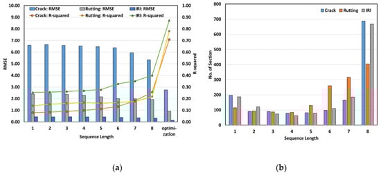
Figure 3.
Scenario analysis: (a) sequence length optimization, (b) number of sections with minimal root-mean-square error (RMSE) for each sequence length.
However, some sections had high prediction performance even in the case of SQL in the range 1–7; this might be because results depended on the deterioration characteristics and the maintenance and repair history. This meant that the SQL required for optimizing each section had to be set differently because the pavement condition index, deterioration characteristics, and maintenance timings differed for each section. In addition, the optimal value of SQL was different for each pavement condition index. This might have been caused by differences in the deterioration speed for each pavement condition.
The above results indicate that the SQL necessary for optimization of each section differed because there were differences in pavement type, traffic loads, and environmental factors of each section. Furthermore, even in the same section, the optimal SQL differed for different pavement condition indices.
Therefore, the optimization process was executed to choose the SQL that would minimize the RMSE for each pavement condition index for each section. The optimization results in Table 6 showe that, compared with a SQL of 1, the RMSE was reduced by 58.3–68.2% and the coefficients of determination (R2) were in the range 0.71–0.87, which represents a high prediction performance. In the case of Rutting depth, R2 was shown to be somewhat lower if SQL was 5, but the overall trend did not exhibit any significant difference. Closer examination reveals that pavement maintenance was implemented based on the Rutting depth index in some sections, which somewhat affected the predictions of SQL 5.
Table 6.
Results of analysis.
5.2. Application of Recurrent Neural Network Models
To evaluate the prediction performance of the RNN algorithm, the pavement condition indices in 2017 predicted by the algorithm and the pavement condition indices measured from the site were directly compared. Figure 4 shows the coefficients of determination for the rutting depth, crack rate, and IRI between the actual measurements and prediction.
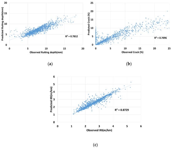
Figure 4.
Coefficient of determination between predicted and actual pavement condition indices: (a) rutting depth, (b) crack, (c) IRI.
In general, the coefficients of determination were in the range 0.71–0.87, indicating that deterioration prediction is possible at a high level of accuracy if the deterioration characteristics in each section are considered. Of the three pavement condition indices, the coefficient of determination for the IRI was the highest, 0.87, while the coefficient of determination for the crack rate was lowest, 0.71. This might be because of high analysis errors or because the IRI and rutting depth were measured automatically by the inspection equipment, whereas the crack rate was measured manually. Additionally, the result mainly depends on the high number of 0 values measured for the crack rate that were not predicted by the RNN model. Despite such errors, even the prediction performance for the crack rate was high, implying the possibility of prediction with a high accuracy.
6. Summary and Concluding Remarks
This study was conducted at Hanbat National University based on data collected by public research institutes and the open-source deep learning framework called TensorFlow to introduce the concept of open innovation to the deep learning field.
This study aimed to predict road pavement deterioration conditions in each RPM section from the RPM data from the Korean NHPMS, using a RNN algorithm. The RNN was implemented using Tensorflow. The algorithm was constructed to predict the pavement condition indices (crack, rutting depth, and IRI) by using the time series data for 10 years (2007–2016) as learning data. The independent variables for analysis were AADT, ESAL, annual average temperature, annual total precipitation, annual maximum temperature, annual minimum temperature, and amount of deicing agent used, and the pavement condition inspection equipment was set as a dummy variable.
In the RNN model, the optimal value of SQL (an important RNN hyperparameter) was determined separately for each section and for each pavement condition index. This is because analysis results showed that the pavement type, traffic loads, and environmental factors were different for each section, and there were differences between the deterioration characteristics of the different pavement condition indices. The optimization process minimized the RMSE by optimizing the SQL for each section and for each pavement condition index. This showed that the RMSE was reduced by 58.3–68.2%, compared with an SQL of 1, while the coefficients of determination were as high as 0.71–0.87, indicating that prediction performance for pavement deterioration is high.
Nevertheless, there are some limitations of this study, as follows.
First, independent variables related to the maintenance history (such as maintenance timing, maintenance method, number of maintenance), service life, and pavement structure that greatly affect the pavement deterioration speed could not be obtained because of missing data. In addition, the RNN algorithm was not optimized by the learning rate, number of epochs, or activation function. However, this study already provided good results by exploiting the road pavement big data and by applying the RNN algorithm to the fields of road property management and road pavement engineering. The results obtained from this study indicate that it is possible to predict pavement deterioration indices with a high degree of accuracy with a RNN algorithm, after SQL is optimized and the characteristics of each section and each pavement deterioration index are considered. Furthermore, because this study uses a new approach, in the form of a RNN algorithm, it could be a basis for future research on the prediction of road pavement deterioration.
Author Contributions
The authors confirm contribution to the paper as follows: Concept idea and design: M.D.; data collection, S.C.; analysis and interpretation of results: M.D. and S.C.; draft manuscript preparation: M.D. and S.C. All authors have read and agreed to the published version of the manuscript.
Funding
This research received no external funding.
Conflicts of Interest
The authors declare no conflict of interest.
References
- Yun, J.; Lee, D.; Ahn, H.; Park, K.; Yigitcanlar, T. Not deep learning but autonomous learning of open innovation for sustainable artificial intelligence. Sustainability 2016, 8, 797. [Google Scholar] [CrossRef]
- Ceylan, H.; Bayrak, M.B.; Gopalakrishnan, K. Neural networks applications in pavement engineering: A recent survey. Int. J. Pavement Res. Technol. 2014, 7, 434–444. [Google Scholar] [CrossRef]
- Saura, J.R.; Debasa, F.; Reyes-Menendez, A. Does User Generated Content Characterize Millennials′ Generation Behavior? Discussing the Relation between SNS and Open Innovation. J. Open Innov. Technol. Market Complex. 2019, 5, 96. [Google Scholar] [CrossRef]
- Saura, J.R.; Reyes-Menendez, A.; Filipe, F. Comparing Data-Driven Methods for Extracting Knowledge from User Generated Content. J. Open Innov. Technol. Market Complex. 2019, 5, 74. [Google Scholar] [CrossRef]
- Yi, C.; Kim, K. A Machine Learning Approach to the Residential Relocation Distance of Households in the Seoul Metropolitan Region. Sustainability 2018, 10, 2996. [Google Scholar] [CrossRef]
- Leikas, J.; Koivisto, R.; Gotcheva, N. Ethical Framework for Designing Autonomous Intelligent Systems, J. Open Innov. Technol. Market Complex. 2019, 5, 18. [Google Scholar] [CrossRef]
- Do, M.; Kwon, S. Selection of Probability Distribution of Pavement Life Based on Reliability Method. Int. J. Highw. Eng. 2010, 12, 61–69. [Google Scholar]
- Mishalani, R.G.; Madanat, S.M. Computation of infrastructure transition probabilities using stochastic duration models. J. Infrastruct. Syst. 2002, 8, 139–148. [Google Scholar] [CrossRef]
- Kobayashi, K.; Kaito, K.; Nam, L. A statistical deterioration forecasting method using hidden Markov model with measurement error. Transp. Res. Part B 2012, 46, 544–561. [Google Scholar] [CrossRef]
- Han, D.; Do, M. Estimation of Life Expectancy and Budget Demands based on Maintenance Strategy. J. Korean Soc. Civil Eng. 2012, 32, 345–356. [Google Scholar] [CrossRef]
- Prozzi, J.A.; Madanat, S.M. Development of pavement performance models by combining experimental and field data. J. Infrastruct. Syst. 2004, 10, 9–22. [Google Scholar] [CrossRef]
- Kim, S.H.; Kim, N. Development of performance prediction models in flexible pavement using regression analysis method. KSCE J. Civil Eng. 2006, 10, 91–96. [Google Scholar] [CrossRef]
- Jiang, Y.; Saito, M.; Sinha, K.C. Bridge performance prediction model using the Markov chain. Transp. Res. Rec. 1988, 1180, 25–32. [Google Scholar]
- Shin, H.C. Development of a semi-parametric stochastic model of asphalt pavement crack initiation. KSCE J. Civil Eng. 2006, 10, 189–194. [Google Scholar] [CrossRef]
- Loizos, A.; Karlaftis, M.G. Prediction of pavement crack initiation from in-service pavements: A duration model approach. Transp. Res. Rec. 2005, 1940, 38–42. [Google Scholar] [CrossRef]
- Kaito, K.; Kobayashi, K. Bayesian estimation of Markov deterioration hazard model. JSCE J. Civil Eng. 2007, 63, 336–355. [Google Scholar] [CrossRef][Green Version]
- Kobayashi, K.; Do, M.; Han, D. Estimation of Markovian transition probabilities for pavement deterioration forecasting. KSCE J. Civil Eng. 2010, 14, 343–351. [Google Scholar] [CrossRef]
- Kobayashi, K.; Kaito, K.; Nam, L.T. A bayesian estimation method to improve deterioration prediction for infrastructure system with Markov chain model. Int. J. Arch. Eng. Constr. 2012, 1, 1–13. [Google Scholar] [CrossRef]
- Han, D.; Kobayashi, K.; Do, M. Section-based multifunctional calibration method for pavement deterioration forecasting model. KSCE J. Civil Eng. 2013, 17, 386–394. [Google Scholar] [CrossRef]
- Han, D.; Kaito, K.; Kobayashi, K. Application of Bayesian estimation method with Markov hazard model to improve deterioration forecasts for infrastructure asset management. KSCE J. Civil Eng. 2014, 18, 2107–2119. [Google Scholar] [CrossRef]
- Attoh-Okine, N.O. Predicting Roughness Progression in Flexible Pavements Using Artificial Neural networks. In Proceedings of the Third International Conference on Managing Pavements, San Antonio, TX, USA, 22–26 May 1994; pp. 55–62. [Google Scholar]
- Attoh-Okine, N.O. Analysis of learning rate and momentum term in backpropagation neural network algorithm trained to predict pavement performance. Adv. Eng. Softw. 1999, 30, 291–302. [Google Scholar] [CrossRef]
- Eldin, N.N.; Senouci, A.B. Condition rating of rigid pavements by neural networks. Can. J. Civil Eng. 1995, 22, 861–870. [Google Scholar] [CrossRef]
- Eldin, N.N.; Senouci, A.B. Use of neural networks for condition rating of jointed concrete pavements. Adv. Eng. Softw. 1995, 23, 133–141. [Google Scholar] [CrossRef]
- Owusu-Ababio, S. Application of Neural Networks to Modeling Thick Asphalt Pavement Performance. In Artificial Intelligence and Mathematical Methods in Pavement and Geomechanical Systems; Attoh-Okine, N.O., Ed.; In Proceedings of the International Symposium, Miami, FL, USA, 5–6 November 1998; CRC Press: Boca Raton, FL, USA, 1998; pp. 23–30. [Google Scholar]
- Lin, J.D.; Yau, J.T.; Hsiao, L.H. Correlation Analysis between International Roughness Index (IRI) and Pavement Distress by Neural Network. In Proceedings of the CD-ROM 82nd annual meeting of the Transportation Research Board, Washington, DC, USA, 12–16 January 2033. [Google Scholar]
- Choi, J.; Adams, T.M.; Bahia, H.U. Pavement roughness modeling using back-propagation neural networks. Comput. Aided Civil Infrastruct. Eng. 2004, 19, 295–303. [Google Scholar] [CrossRef]
- Thube, D.T. Artificial Neural Network (ANN) Based Pavement Deterioration Models for Low Volume Roads in India. Int. J. Pavement Res. Technol. 2012, 5, 115–120. [Google Scholar]
- Gajewski, J.; Sadowski, T. Sensitivity analysis of crack propagation in pavement bituminous layered structures using a hybrid system integrating Artificial Neural Networks and Finite Element Method. Comput. Mater. Sci. 2014, 82, 114–117. [Google Scholar] [CrossRef]
- Kırbaş, U.; Karaşahin, M. Performance models for hot mix asphalt pavements in urban roads. Constr. Build. Mater. 2016, 116, 281–288. [Google Scholar] [CrossRef]
- Choi, S.; Do, M. Prediction of Asphalt Pavement Service Life using a Deep learning. Int. J. Highw. Eng. 2018, 20, 57–65. [Google Scholar] [CrossRef]
- Hinton, G.E.; Osindero, S.; Tech, Y.W. A fast learning algorithm for deep belief nets. Neural Comput. 2006, 18, 1527–1554. [Google Scholar] [CrossRef]
- Dahl, G.E.; Sainath, T.N.; Hinton, G.E. Improving Deep Neural Networks for LVCSR Using Rectified Linear Units and Dropout. In Proceedings of the IEEE International Confedence Acoustics on Speech and Signal Processing(ICASSP), Vancouver, BC, Canada, 26–31 May 2013; pp. 8609–8613. [Google Scholar] [CrossRef]
- Srivastava, N.; Hinton, G.E.; Krizhevsky, A.; Sutskever, I.; Salakhutdinov, R. Dropout: A simple way to prevent neural networks from overfitting. J. Mach. Learn. Res. 2014, 15, 1929–1958. [Google Scholar] [CrossRef]
- Tabatabaee, N.; Ziyadi, M.; Shafahi, Y. Two-stage support vector classifier and recurrent neural network predictor for pavement performance modeling. J. Infrastruct. Syst. 2012, 19, 266–274. [Google Scholar] [CrossRef]
- Okuda, T.; Suzuki, K.; Kohtake, N. Non-Parametric Prediction Interval Estimate for Uncertainty Quantification of the Prediction of Road Pavement Deterioration. In Proceedings of the 2018 21st International Conference on Intelligent Transportation Systems (ITSC), Maui, HI, USA, 4–7 November 2018; pp. 824–830. [Google Scholar] [CrossRef]


© 2019 by the authors. Licensee MDPI, Basel, Switzerland. This article is an open access article distributed under the terms and conditions of the Creative Commons Attribution (CC BY) license (http://creativecommons.org/licenses/by/4.0/).