Current Control Methods for an Asymmetric Six-Phase Permanent Magnet Synchronous Motor

Abstract

Via the vector space decomposition (VSD) transformation, the currents in an asymmetric six-phase permanent magnet synchronous motor (ASP_PMSM) can be decoupled into three orthogonal subspaces. Control of α–β currents in α–β subspace is important for torque regulation, while control of x-y currents in x-y subspace can suppress the harmonics due to the dead time of converters and other nonlinear factors. The zero-sequence components in O₁-O₂ subspace are 0 due to isolated neutral points. In α–β subspace, a state observer is constructed by introducing the error variable between the real current and the internal model current based on the internal model control method, which can improve the current control performance compared to the traditional internal model control method. In x–y subspace, in order to suppress the current harmonics, an adaptive-linear-neuron (ADALINE)-based control algorithm is employed to generate the compensation voltage, which is self-tuned by minimizing the estimated current distortion through the least mean square (LMS) algorithm. The modulation technique to implement the four-dimensional current control based on the three-phase SVPWM is given. The experimental results validate the robustness and effectiveness of the proposed control method.

1. Introduction

Compared to the traditional three-phase motors, multi-phase motors have the advantages of reduced torque ripples and fault tolerant ability [1,2,3,4]. 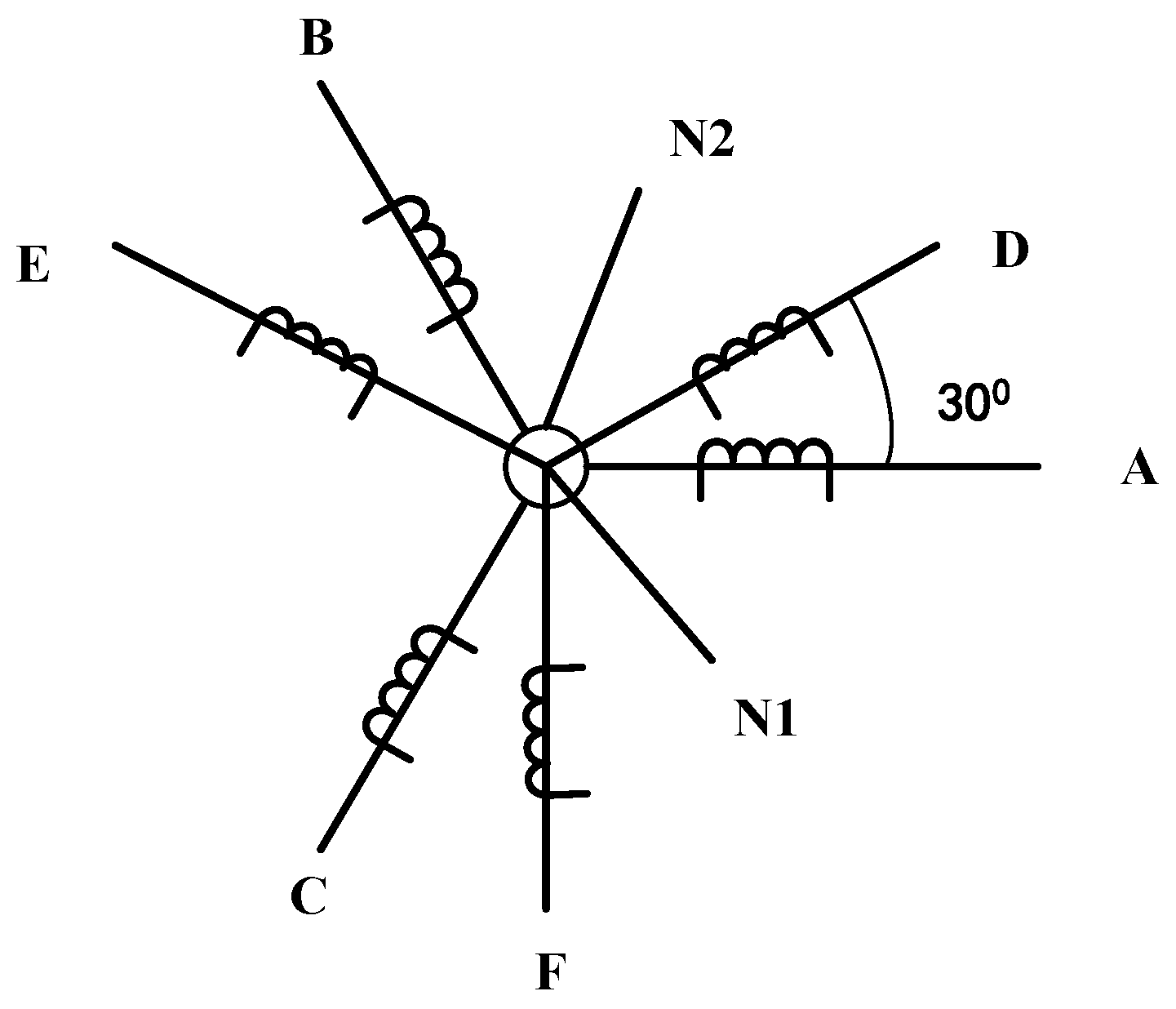Those with multiple three-phase stator windings enjoy popularity among the multi-phase machines (such as six-phase and 15-phase), due to the fact that not only do they have the advantages of multi-phase motors, but also the modular three-phase structures can inherent the use of the well established three-phase topology [1,2]. An asymmetric six-phase permanent magnet synchronous motor (ASP_PMSM) has two sets of three-phase stator windings which are spatially shifted 30 electrical degrees with neutral points being isolated [1], as shown in Figure 1.

In recent years, various research studies related to ASP_PMSM drive system have been studied thoroughly. Two modeling and control methods have been adopted for the ASP_PMSM. They are the double d-q approach [5,6,7] and the vector space decomposition (VSD) approach [8,9,10]. The former scheme has the advantages of modeling and control schemes of traditional three-phase motors and each set of three-phase winding is regarded as a basic unit. It should be remarked that coupling effects exist between two pairs of d-q stator voltage equations, while for the VSD method, two sets of three-phase windings are treated as a whole. All the phase variables can be mapped into three orthogonal subspaces, i.e., α–β subspace, x-y subspace and O₁-O₂ subspace. Only in α–β subspace does the electromechanical energy take place, while the x-y and O₁-O₂ subspaces are only pertinent to the loss. Because the VSD scheme reveals the characteristics of multi-degree freedom for the ASP_PMSM [8,9,10], the current control becomes more flexible compared to the double d-q transformation. Therefore, most of the recent research studies pertinent to ASP_PMSM are based on the VSD method.

Two dimensional current control which only controls the torque producing α–β currents is insufficient [8]. Four-dimensional current control based on the VSD approach can be used not only for torque control but also for the inverter dead time effect [8,9,10,11]. In α–β subspace, the currents are controlled in the rotor coordinates to achieve vector control [8,9,10,11,12,13,14]. This coordinate system is a natural selection because not only are the controllable currents direct currents in steady state but also, the inductance matrix can be decoupled.

Rotor field oriented control (RFOC) is adopted for the motor control in α–β subspace [12,13,14,15,16] because the stator currents can be decomposed into an excitation current component and a torque producing current component which can be controlled separately. Although it offers a lot of advantages, the coupling effects due to the rotating coordinate system exist between the two pairs of voltage equations. In [16,17], a synchronous-frame proportional-integrator (PI) controller which is augmented with the cross-coupling voltage calculated based on the feedback current is adopted. However, when the motor parameters are not well known or vary during operation, the actual currents cannot track the reference currents. The design of a current regulator in a discrete time domain has been discussed by some scholars [17,18], e.g., the Euler or Tustin method. However, the control delay and the characteristics of the inverter are not considered and the proposed design method increases the computation burden and is very complex to design.

In x-y subspace, by applying the duty cycle control strategy, the components which cause loss are eliminated through a suitable selection of virtual voltage vectors [19]. However, the harmonic losses caused by the dead time of converters and the structure of motor itself are not considered. Proportional-Integral (PI) regulators implemented in one positive-sequence synchronous rotating frame (SRF) and one negative-sequence SRF at the same time can be adopted to suppress the current harmonics [20,21,22]. But the multiple coordinate transformations lead to a heavy computational burden and complexity. Accordingly, a resonant controller can be an advantageous alternative [23,24,25,26] to PI regulator in SRF due to the benefits, such as less sensitivity to noise, reduced computational burden and complexity owing to the lack of multiple Park transformations, a lower number of regulators due to the ability to track both positive and negative sequences at the same time. However, phase delay due to the inductive load and the discrepancy between the actual resonant frequency and the desired resonant frequency owing to the discretization are not considered, which will affect the control performance.

This paper proposes current control methods based on VSD transformation for ASP_PMSM. In α–β subspace, internal model control (IMC) with a state observer is adopted to reduce the current fluctuations of d and q axes currents. In x-y subspace, an adaptive-linear-neuron (ADALINE)-based control algorithm is employed to suppress the current harmonics due to the dead time and the non-linearity of the inverter, which is independent of the current polarity and avoids the multiple coordinate transformations compared to the traditional PI controller implemented in one positive-sequence SRF and one negative-sequence SRF at the same time. Moreover, the discretization errors around the resonant frequency can be avoided. The experimental results show that the internal model control (IMC) with the state observer in α–β subspace can reduce the current fluctuations of d and q axes currents compared to the traditional IMC method and the proposed ADALINE algorithm can suppress the current harmonics effectively without the drawbacks compared to the other methods.

This paper is structured as follows. Section 2 gives the relationship between the double dq and VSD model in order to give a detailed explanation of VSD transformation. In Section 3, the current regulator design for α–β subspace is analyzed. A state observer is introduced to improve the robustness against the parametric variations and un-modelled dynamics. In Section 4, an ADALINE-based control algorithm is introduced to suppress the current harmonics. Section 5 gives the PWM techniques for the implementation for the four dimensional current control of ASP-PMSM. The experimental verification is given in Section 6 and the main conclusions are summarized in Section 7.

2. Relationship Between the Double dq and VSD Model

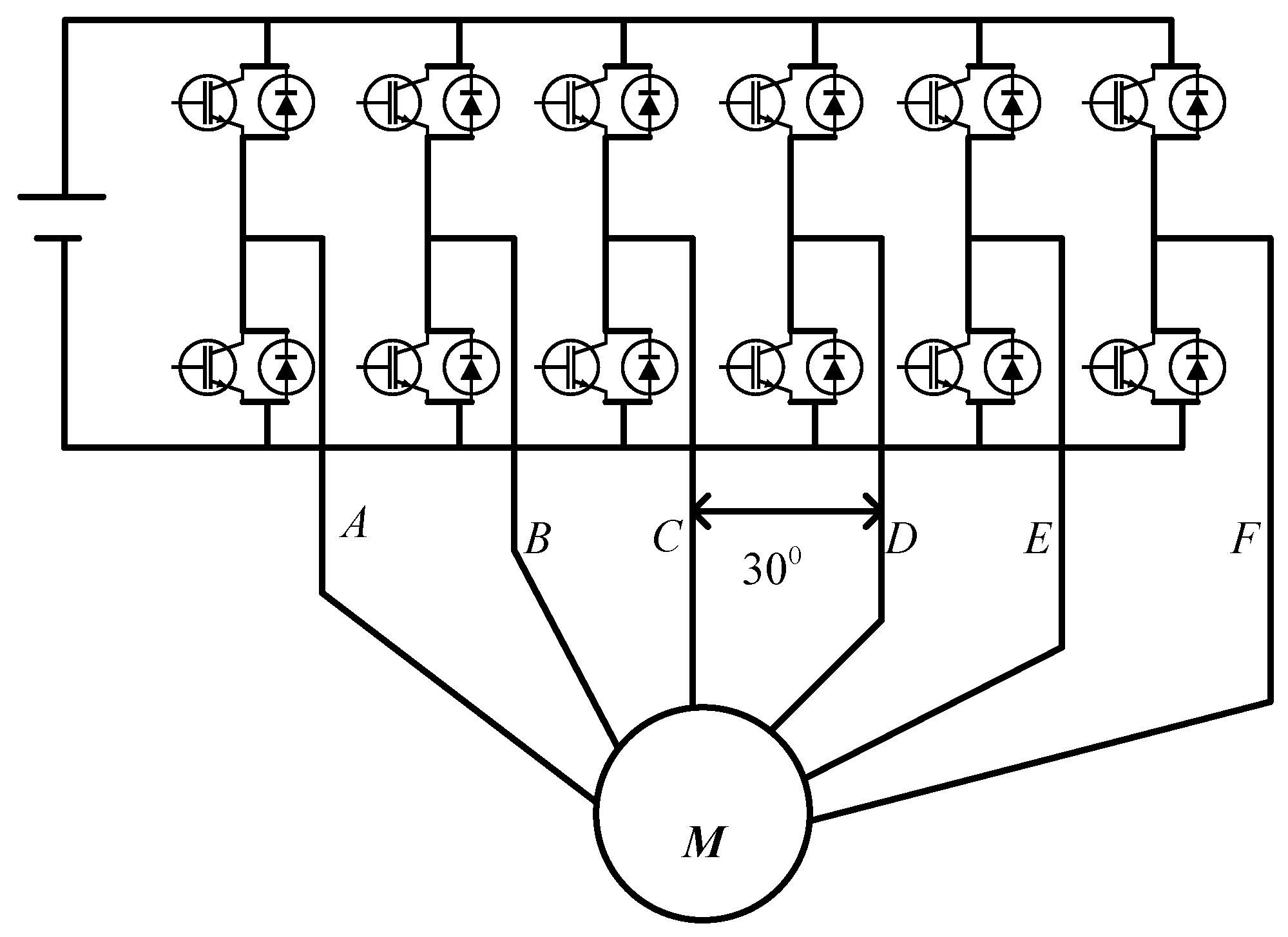
As shown in Figure 2, the drive system of ASP_PMSM, in this paper, has two sets of three-phase VSIs sharing the same dc-link voltage which can supply two sets of three-phase windings.

In the early studies of asymmetrical dual three-phase machines, a double dq or a double stator modelling approach has been utilized to control the motor [5,6,7]. Using this method, two three-phase decoupling (Clarke) transformations are applied separately on the phase variables for each three-phase winding. This transforms the six phase variables into two sets of stationary reference frame variables, which can be denoted as α₁–β₁ and α₂–β₂ components for windings ABC and DEF, respectively.

$${\left[{\begin{array}{cc}{f}_{\alpha 1}& f\end{array}}_{\beta 1}\right]}^T=\left[T_{\alpha \beta 1}\right]{\left[\begin{array}{ccc}{f}_{a1}& f_{b1}& f_{c1}\end{array}\right]}^T$$

(1)

$${\left[{\begin{array}{cc}{f}_{\alpha 2}& f\end{array}}_{\beta 2}\right]}^T=\left[T_{\alpha \beta 2}\right]{\left[\begin{array}{ccc}{f}_{a2}& f_{b2}& f_{c2}\end{array}\right]}^T$$

(2)

Symbol f represents arbitrary machine variables (voltage, current or flux). The spatial 30-degree displacement between the two windings is accounted for in the decoupling transformation. For an asymmetrical six-phase machine, the amplitude invariant transformations for windings 1 and 2 are given with Equations (3) and (4), respectively,

$$\left[T_{\alpha \beta 1}\right]=\frac{2}{3}\left[\begin{array}{ccc}1& -\frac{1}{2}& -\frac{1}{2}\\ 0& \frac{\sqrt{3}}{2}& -\frac{\sqrt{3}}{2}\end{array}\right]$$

(3)

$$\left[T_{\alpha \beta 2}\right]=\frac{2}{3}\left[\begin{array}{ccc}\frac{\sqrt{3}}{2}& -\frac{\sqrt{3}}{2}& 0\\ \frac{1}{2}& \frac{1}{2}& -1\end{array}\right]$$

(4)

while VSD provides an alternative approach for describing the operation of a six-phase machine. Using the VSD model, a six-phase machine can be represented via three orthogonal subspaces [8,9,10], i.e., the α–β, x–y, and zero-sequence subspaces. This approach gives an alternative description of the machine, which is useful for machine control and the development of pulse width modulation (PWM) techniques. After the VSD transformation, harmonics of different orders are mapped into different subspaces. The fundamental component and harmonics with the order 12n ± 1(n = 1, 2, 3 …) are mapped into the α–β subspace. The harmonics with the order 6n ± 1(n = 1, 3, 5 …) are mapped into the x–y subspace. The harmonics with the order 6n ± 3(n = 1, 3, 5 …) are mapped into the O₁–O₂ subspace, i.e., the zero sequence subspace. With the neutral points being isolated, no current components in the O₁–O₂ subspace would exist. Therefore, the ASP_PMSM with the isolated neutrals is a four-order system. The mathematical model and the VSD modelling process of the dual three-phase motor are described in more detail in [8,9,10]. The static decoupling transformation matrix is

$$T_{\alpha \beta }=\frac{1}{3}\left[\begin{array}{cccccc}1& -\frac{1}{2}& -\frac{1}{2}& \frac{\sqrt{3}}{2}& -\frac{\sqrt{3}}{2}& 0\\ 0& -\frac{\sqrt{3}}{2}& \frac{\sqrt{3}}{2}& \frac{1}{2}& \frac{1}{2}& -1\\ 1& -\frac{1}{2}& -\frac{1}{2}& -\frac{\sqrt{3}}{2}& \frac{\sqrt{3}}{2}& 0\\ 0& -\frac{\sqrt{3}}{2}& \frac{\sqrt{3}}{2}& \frac{1}{2}& \frac{1}{2}& -1\end{array}\right]$$

(5)

Despite the various advantages of the VSD model, the variables are more difficult to interpret physically, unlike in the double dq model where α₁–β₁ variables are clearly related to the winding 1 and α₂–β₂ variables to the winding 2 of the machine. It is therefore desirable to provide a better physical interpretation of the VSD model variables by relating them with variables in the double dq model. This can be done by simply comparing the decoupling transformation matrices for the two methods. By comparing Equations (3)–(5), it can be seen that the α component in the VSD model is proportional to the sum of the α₁ and α₂ components. The β component in the VSD model is proportional to the sum of the β₁ and β₂ components of the double dq model. On the other hand, the x component is proportional to the difference between the α₁ and α₂ components, while the y component is proportional to the difference between the β₁ and β₂ components with the signs for the x and y components being inverted. As will be shown later, this opposite sign influences the rotational direction of the x–y current phasor caused by the converter asymmetry. The relationship is given with

$$\begin{array}{l}{f}_{\alpha }=\frac{1}{2}(f_{\alpha 1}+f_{a2})\\ f_{\beta }=\frac{1}{2}(f_{\beta 1}+f_{\beta 2})\\ f_x=\frac{1}{2}(f_{\alpha 1}-f_{a2})\\ f_y=-\frac{1}{2}(f_{\beta 1}-f_{\beta 2})\end{array}$$

(6)

The fifth and seventh current harmonics in windings 1 and 2 can be represented as

$$\begin{array}{l}{\overrightarrow{I}}_{\alpha \beta 1}^h=k_{1}I{e}^{-5j{w}_{e}t}+k_{2}I{e}^{7j{w}_{e}t}\\ {\overrightarrow{I}}_{\alpha \beta 2}^h=k_{3}I{e}^{-5j{w}_{e}t}+k_{4}I{e}^{7j{w}_{e}t}\end{array}$$

(7)

where k₁ and k₂ are the weights of the fifth and seventh current harmonics in winding 1, while k₃ and k₄ are the weights of the fifth and seventh current harmonics in winding 2. w_e is the electrical angular speed.

According to Equations (6) and (7), the expression of x-y currents can de deduced as

$${\overrightarrow{I}}_{xy}^h=(k_1-k_3)I{e}^{5j{w}_{e}t}+(k_2-k_4)I{e}^{-7j{w}_{e}t}$$

(8)

It is worth noting that the rotational direction of the current harmonics has changed due to the opposite polarity in the x-y currents. Therefore, the positive sequence component in α–β subspace will become the negative sequence component in x-y subspace, and vice versa.

Since only the components in the α–β subspace are related to electromechanical energy conversion, it is only necessary to transform α–β components into the general synchronous reference frame d–q components. The x–y subspace can remain in the stator-fixed coordinate system. The rotating transformation matrix is

$$T_r=\left[\begin{array}{ccc}\cos \theta & \sin \theta & 0\\ -\sin \theta & \cos \theta & 0\\ 0& 0& I_2\end{array}\right]$$

(9)

where θ is the electrical rotor position, I₂ is a two-dimensional unit matrix, and the transformation matrix T between the original phase-variable (ABC, DEF) and the variables after rotating coordinates (d–q, x–y) is defined as

$$T=T_r\ast T_{\alpha \beta }$$

(10)

The voltage, flux, and torque equations are shown in Equations (11)–(13) respectively.

$$\left[\begin{array}{c}{u}_d\\ u_q\\ u_x\\ u_y\end{array}\right]=\left[\begin{array}{cccc}R& 0& 0& 0\\ 0& R& 0& 0\\ 0& 0& R& 0\\ 0& 0& 0& R\end{array}\right]\left[\begin{array}{c}{i}_d\\ i_q\\ i_x\\ i_y\end{array}\right]+\frac{d}{dt}\left[\begin{array}{c}{\psi }_d\\ {\psi }_q\\ {\psi }_x\\ {\psi }_y\end{array}\right]+w\left[\begin{array}{c}-{\psi }_q\\ {\psi }_d\\ 0\\ 0\end{array}\right]$$

(11)

$$\left[\begin{array}{c}{\psi }_d\\ {\psi }_q\\ {\psi }_x\\ {\psi }_y\end{array}\right]=\left[\begin{array}{cccc}{L}_d& 0& 0& 0\\ 0& L_q& 0& 0\\ 0& 0& L_z& 0\\ 0& 0& 0& L_z\end{array}\right]\left[\begin{array}{c}{i}_d\\ i_q\\ i_x\\ i_y\end{array}\right]+\left[\begin{array}{c}{\psi }_f\\ 0\\ 0\\ 0\end{array}\right]$$

(12)

$$T_e=3p\left[\left(L_d-L_q\right)i_d{i}_q+{\psi }_f{i}_q\right]$$

(13)

where L_d, L_q are d-q axes inductances, and L_z is stator self-leakage inductance. P is the number of pole pairs. ψ_f is the permanent magnet flux linkage.

3. Current Control Method in α–β Subspace

3.1. Internal Model Control Method

The principle of internal model control is shown Figure 3. G(s) is the plant model, $\widehat{G}$(s) is the internal model and C(s) is the internal current controller.

Assuming that the internal model is exact, i.e., $\widehat{G}$(s) = G(s). Then, the transfer function of the system is

$$G_c(s)=C(s)G(s)$$

(14)

The dotted line part can be represented by F(s), as follows:

$$F(s)=\frac{U(s)}{E(s)}=\frac{C(s)}{I-C(s)\widehat{G}(s)}$$

(15)

Since the controlled plant is a first-order system, according to the principle of internal model control, C(s) can be defined as follows:

$$C(s)={\widehat{G}}^{-1}(s)L(s)=G^{-1}(s)L(s)$$

(16)

where L(s) is a first-order low pass filter, which can be represented as follows:

$$L(s)=\frac{1}{\lambda s+1}$$

(17)

where λ is the time constant.

Substituting Equations (16) and (17) into Equation (15), the current controller can be obtained as follows:

$$F(s)=\frac{1}{\lambda }\left[\begin{array}{cc}{L}_d(1+\frac{R}{s{L}_d})& 0\\ 0& L_q(1+\frac{R}{s{L}_q})\end{array}\right]$$

(18)

The closed-loop transfer function is

$$G_c(s)=\frac{1}{\lambda s+1}I$$

(19)

Compared with the traditional Proportional-Integral (PI) regulator, the regulation parameters are reduced from two to one, and the system is naturally stable without overshoot. The response speed of the system is directly related to λ. The response speed is faster with the decrease of λ. However, λ cannot decrease indefinitely due to the delay of the converter.

3.2. State Observer Based on The Internal Model Control

The parameters of the motor may vary depending on their designed values. However, the accuracy of the model depends on the parameters of the system. The parametric variations of R, L_d, L_q and ψ_f can be defined as ΔR, ΔL_d, ΔL_q and Δψ_f. Therefore, the voltage equation in α–β subspace can be rewritten as

$$\{\begin{array}{c}{u}_d=R{i}_d+L_d\frac{d{i}_d}{dt}-w_e{L}_q{i}_q+{\sigma }_d\\ u_q=R{i}_q+L_q\frac{d{i}_q}{dt}+w_e(L_d{i}_d+{\psi }_f)+{\sigma }_q\end{array}$$

(20)

where σ_d and σ_q are the uncertainties of the d and q-axis voltage equations, which can be defined as

$$\{\begin{array}{c}{\sigma }_d=\mathsf{\Delta }R{i}_d+\mathsf{\Delta }{L}_d\frac{d{i}_d}{dt}-\mathsf{\Delta }{L}_q{w}_e{i}_q+{\epsilon }_d\\ {\sigma }_q=\mathsf{\Delta }R{i}_q+\mathsf{\Delta }{L}_q\frac{d{i}_q}{dt}+\mathsf{\Delta }{L}_d{w}_e{i}_d+w_e\mathsf{\Delta }{\psi }_f+{\epsilon }_d\end{array}$$

(21)

where ε_d and ε_q are un-modelled dynamics, including the flux harmonics.

Taking the q-axis voltage in Equation (20), for example, which can be described by the state equation as follows

$$\dot{x}=ax+b(u-d)$$

(22)

where $x=i_q;\hspace{1em}u=u_q-u_1;\hspace{1em}{u}_1=w_e{L}_d{i}_d+w_e{\psi }_f;\hspace{1em}a=-R/L_q;\hspace{1em}b=1/L_q$ the state estimation voltage equation of q-axis is

$$\dot{\widehat{x}}=a\widehat{x}+b(u-\widehat{d})$$

(23)

where $\widehat{x}$ and $\widehat{d}$ are the estimated parameter values of x and d, respectively.

The deviation value between the estimated and real values can be defined as

$$\tilde{x}=x-\widehat{x}=i_q-\widehat{i_q};\begin{array}{cc}& \tilde{d}=d-\widehat{d}\end{array}$$

(24)

By using Equations (22)–(24), the new state equation is

$$\{\begin{array}{l}\dot{\tilde{x}}=a\tilde{x}+b\tilde{d}\\ y=\tilde{x}\end{array}$$

(25)

Equation (25) denotes the error state equation between the estimation and the actual plant. Assuming that the reference input is 0 and $\tilde{d}$ can be assumed as the control variable to be designed, the tracking error e of Equation (25) is

$$\{\begin{array}{l}e=0-y\\ \dot{e}=-\dot{y}=-\dot{\tilde{x}}\end{array}$$

(26)

Two new state variables z and m are introduced, which can be given as

$$\{\begin{array}{l}z=\dot{\tilde{x}}\\ m=\dot{\tilde{d}}\\ \dot{z}=\ddot{\tilde{x}}=az+bm\end{array}$$

(27)

According to Equations (25)–(27), the extended system equation can be given as

$$\left[\begin{array}{l}\dot{e}\\ \dot{z}\end{array}\right]=\left[\begin{array}{cc}0& -1\\ 0& a\end{array}\right]\left[\begin{array}{c}e\\ z\end{array}\right]+\left[\begin{array}{c}0\\ b\end{array}\right]m\to \dot{Z}=AZ+Bm$$

(28)

where $A=\left[\begin{array}{cccc}0& -1& 0& a\end{array}\right],{\begin{array}{cc}& B=\left[\begin{array}{cc}0& b\end{array}\right]\end{array}}^T,\begin{array}{cc}& m=-KZ,\begin{array}{cc}& K=\left[\begin{array}{cc}{k}_1& k_2\end{array}\right]\end{array}\end{array}$.

It is apparent that the rank of the matrix $\left[\begin{array}{cc}B& AB\end{array}\right]$ is 2, i.e., rank $\left[\begin{array}{cc}B& AB\end{array}\right]=2$, which indicates that Equation (28) is fully controllable. According to the principle of the state feedback control theory, the controllable variable is

$$\dot{\tilde{d}}=m=-k_{1}e-k_{2}z=-k_1\tilde{x}-k_2\dot{\tilde{x}}$$

(29)

where k₁ and k₂ are the parameters to be set. Assuming that d is constant during one PWM period, which means that the $\dot{d}$ = 0, equation can be further expressed as

$$\dot{\widehat{d}}=k_1\tilde{x}-k_2\dot{\tilde{x}}$$

(30)

The roots of state feedback system can be obtained by Equation (31)

$$\det \left[SI-(A-BK)\right]=0$$

(31)

According to the Hurwitz stability criterion, the ranges of k₁ and k₂ are

$$k_1<0;\begin{array}{cc}& k_2>\frac{a}{b}\end{array}$$

(32)

The observer parameters k₁ and k₂ can be optimized by using the distribution of eigenvalues of standard second-order oscillatory systems.

$$k_1=-\frac{w_n^2}{b};\begin{array}{cc}& k_2=\frac{a+2\xi w_n^2}{b}\end{array}$$

(33)

where ξ and w_n are the damping ratio and the angular frequency of natural oscillation. By setting the parameters of the standard second-order system and pole placement, the optimal control quantity can be obtained.

The observer for d-axis can be obtained in a similar way. The block diagram for the state observer based on internal model control is shown in Figure 4.

4. Current Control Method in x-y Subspace

A feedback current control loop is adopted in x-y subspace to suppress the sixth order current harmonics. An ADALINE-based voltage compensator based on the least mean square (LMS) algorithm is used to generate the compensating voltage.

As discussed in Section 2, the signs of the fifth and seventh current harmonics are inverted, which will appear as +fifth and −seventh in the x-y subspace. The +fifth and -seventh harmonic currents will become +sixth and −sixth, respectively, after the inverse Park transformation. Thus, an ADALINE-based voltage compensator should be implemented in the synchronous frame rotating at −w_e (clockwise rotation) which can be defined as the x1-y1 coordinate axis in order to eliminate the sixth current harmonics. Thus, the sixth current harmonics in the x1-y1 coordinate axis can be defined as follows:

$$\left[\begin{array}{c}{I}_{x1}^6\\ I_{y1}^6\end{array}\right]=\left[\begin{array}{c}{I}_{xs}\sin (6w_{e}t)+I_{xc}\cos (6w_{e}t)\\ I_{ys}\sin (6w_{e}t)+I_{yc}\cos (6w_{e}t)\end{array}\right]$$

(34)

In order to reduce the current harmonics in x-y subspace, the desired current harmonics in x-y subspace should be 0. Let the compensation voltage vector on the x1-y1 coordinate axis be defined as

$$\left[\begin{array}{c}{u}_{x1}^{com}\\ u_{y1}^{com}\end{array}\right]=\left[\begin{array}{c}{u}_{xs}\sin (6w_{e}t)+u_{xc}\cos (6w_{e}t)\\ u_{ys}\sin (6w_{e}t)+u_{yc}\cos (6w_{e}t)\end{array}\right]$$

(35)

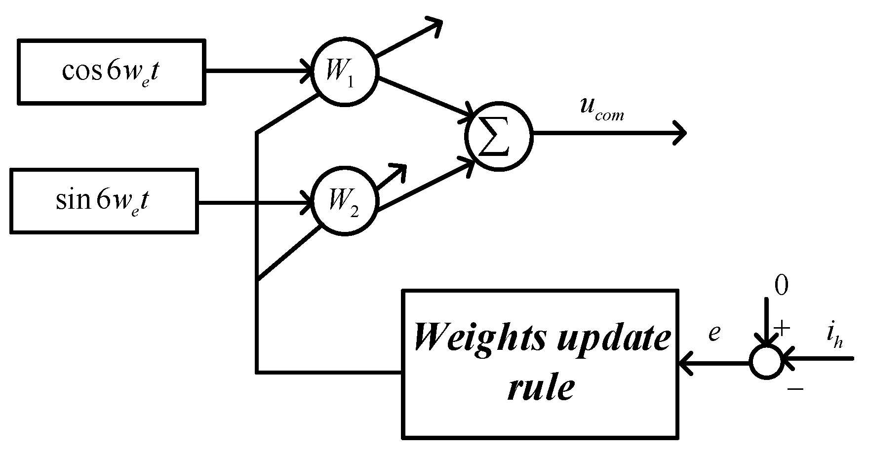
The ADALINE network is an efficient scheme in detecting harmonics, which can also track the harmonic components with satisfactory performance due to the characteristics of the supervised learning mechanism. The block diagram is shown in Figure 5. It should be remarked that the ADALINE-based algorithm is a single-layer linear neural element which is trained online according to the input signals, the target response and the weight updating rule.

u_com can be calculated as

$$u_{com}=X^T\ast W$$

(36)

where X denotes the reference input vector, which is calculated by taking the cosine and sine terms of the six times of the electric rotor position θ. W is the adjustable weight vector.

$$X={\left[\begin{array}{cc}\cos 6w_{e}t& \sin 6w_{e}t\end{array}\right]}^T\hspace{1em}W={\left[\begin{array}{cc}{W}_1& W_2\end{array}\right]}^T$$

(37)

For illustration purposes, the x1-axis is analyzed in detail. The u_x1^com in Equation (37) can be rewritten in vector form described as

$$u_{x1}^{com}=\left[\begin{array}{cc}\sin 6w_{e}t& \cos 6w_{e}t\end{array}\right]\left[\begin{array}{c}{u}_{xs}^{com}\\ u_{ys}^{com}\end{array}\right]=X^T\ast W$$

(38)

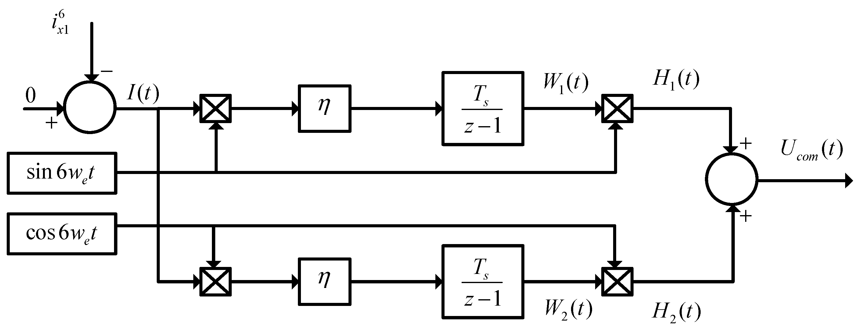
The least mean square (LMS) algorithm is very popular for the ADALINE, which has the advantages of a simple structure and easy implementation. For illustration purposes, the x1-axis is analyzed in detail. The block diagram of the ADALINE algorithm based on the LMS algorithm is shown in Figure 6.

In terms of classical control, W₁(Z) in the Z-domain can be expressed as

$$\begin{array}{l}{W}_1(z)=\frac{T_s}{z-1}Z(\eta I(t)\sin 6w_{e}t)\\ =\frac{\eta T_s}{z-1}Z[I(t)\frac{1}{2j}(e^{j6w_{e}t}-e^{-j6w_{e}t})]\\ =\frac{\eta T_s}{2j}\frac{1}{z-1}Z(I(z{e}^{-j6w_e{T}_s})-I(z{e}^{-j6w_e{T}_s}))\end{array}$$

(39)

where η is the learning rate and Z () is the Z-transform.

H₁(t) can be expressed as

$$h_1(t)=W_1(t)\sin 6w_{e}t=W_1(t)\frac{1}{2j}(e^{j6w_{e}t}-e^{-j6w_{e}t})$$

(40)

Transforming H₁(t) into Z-domain, H₁(Z) can be obtained as

$$\begin{array}{l}{H}_1(Z)=\frac{1}{2j}(W_1(z{e}^{-j6w_e{T}_s})-W(z{e}^{j6w_e{T}_s}))\\ =-\frac{\eta T_s}{4}\frac{1}{z{e}^{-j6w_e{T}_s}-1}(I(z{e}^{-j12w_e{T}_s})-I(z))+\frac{\eta T_s}{4}\frac{1}{z{e}^{j6w_e{T}_s}-1}(I(z)-I(z{e}^{j12w_e{T}_s}))\end{array}$$

(41)

Similarly, H₂(Z) can be obtained as follows

$$\begin{array}{l}{H}_2(Z)=\frac{1}{2}(W_2(z{e}^{-j6w_e{T}_s})+W_2(z{e}^{j6w_e{T}_s}))\\ =\frac{\eta T_s}{4}\frac{1}{z{e}^{-j6w_e{T}_s}-1}(I(z{e}^{-j12w_e{T}_s})+I(z))+\frac{\eta T_s}{4}\frac{1}{z{e}^{j6w_e{T}_s}-1}(I(z)+I(z{e}^{-j12w_e{T}_s}))\end{array}$$

(42)

U_com(Z) can be calculated as

$$U_{com}(Z)=H_1(Z)+H_2(Z)$$

(43)

The closed loop transfer function of ADALINE based on the LMS algorithm is

$$G_{LMS}(Z)=\frac{U_{com}(Z)}{I(Z)}=\eta T_s\frac{z\cos 6w_e{T}_s-1}{z^2-2z\cos 6w_e{T}_s+1}$$

(44)

From the aforementioned analysis, the ADALINE based on the LMS algorithm is equivalent to the resonant controller with resonant frequency adaption. It can achieve infinite gain at a specific frequency. Moreover, it can avoid the multiple coordinate transformations of the PI controller implemented in one positive-sequence SRF and one negative-sequence SRF at the same time. Compared to the resonant controller, the discretization errors around the resonant frequency can be avoided. 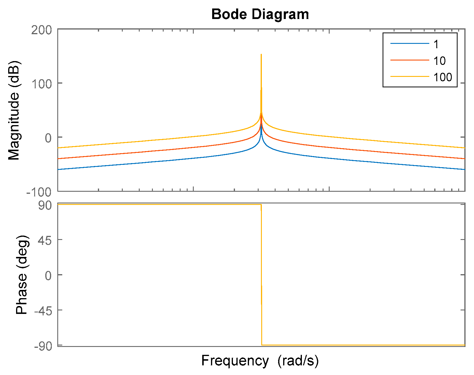Figure 7 depicts the bode diagram with different η values (1, 10,100) of ADALINE based on the LMS algorithm. The convergence speed of the controller increases as η increases, but this will influence frequency selection characteristics and amplify the noises. In addition, it can be seen from the Bode diagram that the phase lag around the frequency to be suppressed is 90 degrees, which is far from 180 degrees and ensures the stability of the ADALINE-based control algorithm.

5. PWM Techniques for Four Dimensional Current Control of ASP_PMSM

The reference voltages in the α–β and x-y subspaces need to be synthesized simultaneously in order to realize the four-dimensional current control. The three-phase decoupling PWM strategy can decompose the voltage vector of six-phase voltage source inverter into two vectors of two three-phase voltage source inverters with a 30 degrees phase shift. Therefore, the three-phase SVPWM algorithm can be adopted to implement four-dimensional current control [26].

The six-phase inverter can be viewed as two independent three-phase inverters with a 30-degree phase shift. In terms of Equations (1) and (2) the reference voltage vectors of the two independent three-phase inverters can be defined as

$$\overrightarrow{u_{\alpha \beta 1}}=u_{a1}+j{u}_{\beta 1}–\overrightarrow{u_{\alpha \beta 2}}=u_{a2}+j{u}_{\beta 2}$$

(45)

where $\overrightarrow{u_{\alpha \beta 1}}$ and $\overrightarrow{u_{\alpha \beta 2}}$ denote the voltage vector of ABC and DEF windings, respectively. $u_{\alpha 1}$ and $u_{\beta 1}$ are the α–β voltage components in the ABC windings, while $u_{\alpha 2}$ and $u_{\beta 2}$ are the α–β voltage components in the DEF windings.

The reference voltage vectors in α–β and x-y subspaces can be represented as

$$\overrightarrow{u_{\alpha \beta }}=u_{\alpha }+j{u}_{\beta }=u_{\alpha 1}+u_{\alpha 2}+j(u_{\beta 1}+u_{\beta 2})$$

(46)

$$\overrightarrow{u_{xy}}=u_x+j{u}_y=u_{\alpha 1}-u_{\alpha 2}-j(u_{\beta 1}-u_{\beta 2})$$

(47)

where $\overrightarrow{u_{\alpha \beta }}$ and $\overrightarrow{u_{xy}}$ denote the voltage vectors in the α–β and x-y subspaces, respectively. It should be remarked that the signs for the x-y components are inverted.

In terms of Equations (46) and (47), the relationship between the voltage vectors of the six-phase inverter and the three-phase inverter is shown as follows

$$\overrightarrow{u_{\alpha \beta 1}}=\overrightarrow{u_{\alpha \beta }}+\overrightarrow{u_{xy}^{\ast }}\hspace{1em}\overrightarrow{u_{\alpha \beta 2}}=e^{-j{30}^0}(\overrightarrow{u_{\alpha \beta }}-\overrightarrow{u_{xy}^{\ast }})$$

(48)

where $\overrightarrow{u_{xy}^{*}}$ is the conjugate function of $\overrightarrow{u_{xy}}$.

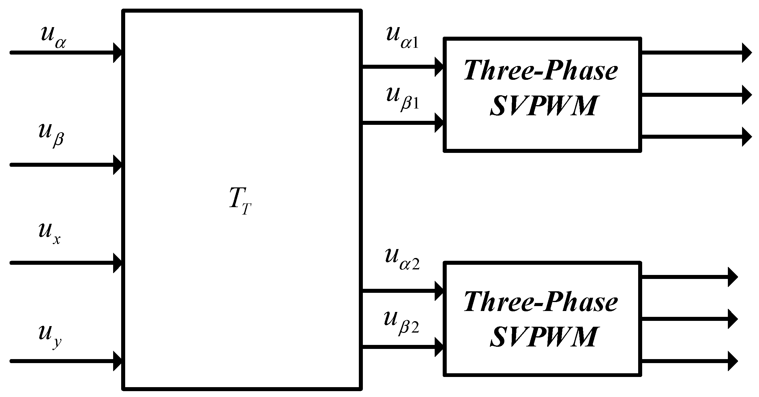
Equation (48) can be rewritten in the matrix form shown below

$${\left[\begin{array}{cccc}{u}_{\alpha 1}& u_{\beta 1}& u_{\alpha 2}& u_{\beta 2}\end{array}\right]}^T=T_T{\left[\begin{array}{cccc}{u}_{\alpha }& u_{\beta }& u_x& u_y\end{array}\right]}^T$$

(49)

where T_T is

$$T_T=\left[\begin{array}{cccc}1& 0& 1& 0\\ 0& 1& 0& -1\\ \frac{\sqrt{3}}{2}& \frac{1}{2}& -\frac{\sqrt{3}}{2}& \frac{1}{2}\\ -\frac{1}{2}& \frac{\sqrt{3}}{2}& \frac{1}{2}& \frac{\sqrt{3}}{2}\end{array}\right]$$

(50)

From Equations (49) and (50), it is obvious that the traditional three-phase SVPWM can be adopted. The implementation of PWM for ASP_PMSM is shown in Figure 8.

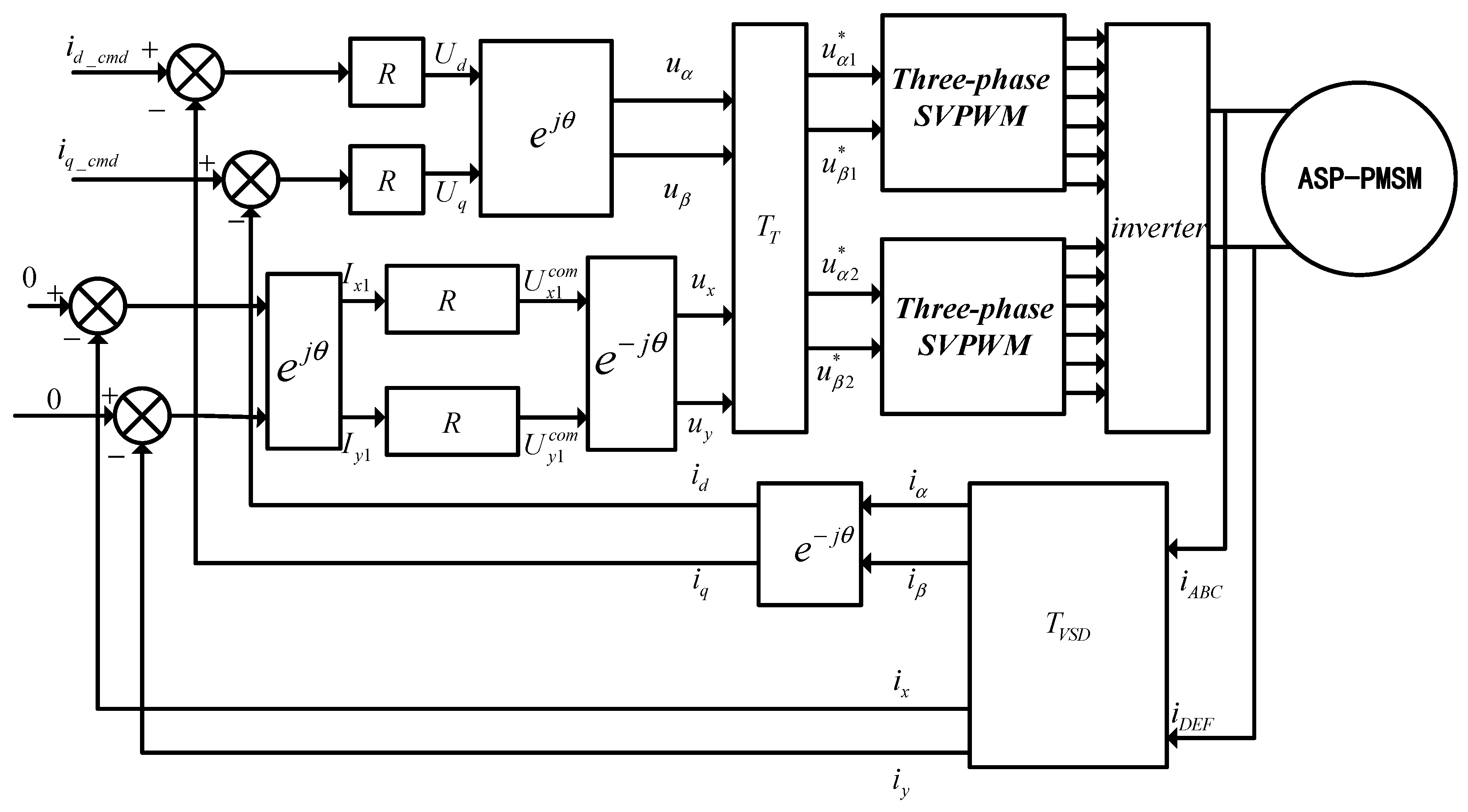
From the above analysis, the proposed current control scheme is divided into two parts, including four independent current components and PWM implementation, as depicted in Figure 9.

6. Experimental Verification

The effectiveness of the proposed method is verified by the implementation in an ASP-PMSM experimental set-up. The experimental set-up is shown in Figure 10, which is composed of a dc-machine mechanically coupled to the ASP_PMSM acting as a loading motor. The loading motor is controlled in speed control mode. The ASP_PMSM is supplied by using a two-level voltage source inverter (VSI), configured for six-phase operation. A dc power supply is used to provide the dc-link voltage of 12 V to the VSI. The complete control algorithm was implemented in a control board using Infineon TC277. The switching frequency is 20 kHz with 1 μs dead time provided by the hardware in the VSI. For variables such as d–q currents, the values are saved as Excel files with the help of control board. To provide the current display at a higher resolution, a current probe (CP150) and a Teledyne Lecroy oscilloscope (WaveSurfer 3024) were used. The data of the phase currents were saved as Excel files with the help of the oscilloscope.

The parameters for ASP-PMSM are given in

Table 1. Machine parameters.

Parameter, Unit	Value
Inductance Value d, H	0.00008
Inductance Value q, H	0.00008
Leakage inductance Value, H	0.000072
Flux, Wb	0.005
Pole Pairs	4
Resistance, Ω	0.0113

.

6.1. Verification of Current Control Method in α–β Subspace

Performances are compared with and without the state observer in α–β subspace. In the experiments, the ASP_PMSM speed is set by the active dynamometer. k₁ and k₂ are set to −32,000 and 50, respectively. The test procedure is to input command currents and then observe the current responses. The command currents for id and iq are 0 A and 20 A, respectively. In order to test the robustness against the uncertainty capability of the current control scheme, controllers designed in α–β subspace are based on the group of virtual parameters R’ = 0.6R, L_d’ = 0.6L_d, L_q’ = 0.7L_q, ψ’ = 0.6ψ_f. It is obvious that the experimental ASP_PMSM operates with parametric uncertainties of 0.4R, 0.4L_d, 0.3L_q, and 0.4ψ_f. Figure 11 shows the experimental results by using the traditional IMC without a state observer. Figure 12 shows the results after adopting the proposed state observer. By employing the traditional IMC, although it can track the reference current, the large current fluctuations are unavoidable because the variations of the parameters and the un-modelled dynamics are not considered. While the IMC with the state observer shows better control performances, the current fluctuations are smaller than that by using IMC without the state observer.

6.2. Verification of Current Control Method in x-y Subspace

To demonstrate the effectiveness of the proposed control algorithm in x-y subspace to eliminate the current harmonic components, experiments with and without ADALINE algorithm were conducted. The learning rate η was chosen as 10. Figure 13 shows the experimental results of phase A and D currents without employing the ADALINE-based voltage compensator when the ASP_PMSM is operating in the current control loop, while the speed is set as 500 rpm by the loading motor. The total harmonic distortion is 24.14%.

Figure 14 shows the experimental results of phase A and D currents without employing the ADALINE-based voltage compensator when the ASP_PMSM is operating in the current control loop, while the speed is set to 1500 rpm by the loading motor. The total of harmonic distortions is 16.18%. Without the closed loop control strategy in x-y subspace, the phase currents are severely distorted because of the dead time effects and other nonlinear factors. Moreover, it can be seen that the system is more sensitively influenced by the error voltage at low speed than at high speed.

Figure 15 and Figure 16 give the experimental results after employing the ADALINE-based voltage compensator when the ASP_PMSM is operating in the current control loop while the speed is set to 500 rpm and 1500 rpm, respectively, by the loading motor. It can be seen that the harmonic currents can be eliminated effectively, which improves the quality of waveform. The total harmonic distortions are reduced to 4.46% and 3.25%.

7. Conclusions

This paper proposes current control methods for ASP-PMSM based on the VSD transformation. In α–β subspace, in order to improve the robustness against parametric variations and un-modelled dynamics, a state-space model for current loops was set up as an internal model and a state observer to estimate the uncertainties was constructed by introducing the error variable between a real current and the estimated current. Then, a control law for the state observer was derived by the state feedback control theory. Finally, the observer parameters were optimized by the pole placement. In x–y subspace, in order to suppress the current harmonics caused by the dead time of the converter and motor structure itself, a new synchronous rotating coordinate matrix is proposed, based on which an adaptive-linear-neuron-based control algorithm was adopted to generate the compensation voltage, which was self-tuned by minimizing the estimated current distortion through the LMS algorithm. The experimental results verify the robustness and effectiveness of the proposed control methods.

Future work will focus on suppressing the current harmonics to an even smaller THD value through the dead time compensation method as feedforward compensation combined with the ADALINE-based control algorithm acting as the feedback control.

References

1. Zheng, J.; Huang, S.; Rong, F.; Lye, M. Six-Phase Space Vector PWM under Stator One-Phase Open-Circuit Fault Condition. Energies 2018, 11, 1796. [Google Scholar] [CrossRef] [Green Version]
2. Levi, E. Multiphase Electric Machines for Variable-Speed Applications. IEEE Trans. Ind. Electron. 2008, 55, 1893–1909. [Google Scholar] [CrossRef]
3. Kamel, T.; Abdelkader, D.; Said, B.; Padmanaban, S.; Iqbal, A. Extended Kalman Filter Based Sliding Mode Control of Parallel-Connected Two Five-Phase PMSM Drive System. Electronics 2018, 7, 14. [Google Scholar] [CrossRef] [Green Version]
4. Levi, E.; Bojoi, R.; Profumo, F.; Toliyat, H.; Williamson, S.; Bojoi, I.R. Multiphase induction motor drives—A technology status review. IET Electr. Power Appl. 2007, 1, 489. [Google Scholar] [CrossRef] [Green Version]
5. Bojoi, R.; Profumo, F.; Tenconi, A. Digital synchronous frame current regulation for dual three-phase induction motor drives. In Proceedings of the IEEE 34th Annual Conference on Power Electronics Specialist, 2003. PESC ’03, Acapulco, Mexico, 15–19 June 2003. [Google Scholar]
6. Lipo, T.A. A d-q model for six phase induction machines. Proc. Int. Conf. Electr. Mach. 1980, 2, 860–867. [Google Scholar]
7. Singh, G.K.; Nam, K.; Lim, S.K. A Simple Indirect Field-Oriented Control Scheme for Multiphase Induction Machine. IEEE Trans. Ind. Electron. 2005, 52, 1177–1184. [Google Scholar] [CrossRef]
8. Ahmad, M.; Wang, Z.; Yan, S.; Wang, C.; Wang, Z.; Zhu, C.; Qin, H. Comparative Analysis of Two and Four Current Loops for Vector Controlled Dual-Three Phase Permanent Magnet Synchronous Motor. Electronics 2018, 7, 269. [Google Scholar] [CrossRef]
9. Zhao, Y.; Lipo, T. Space vector PWM control of dual three-phase induction machine using vector space decomposition. IEEE Trans. Ind. Appl. 1995, 31, 1100–1109. [Google Scholar] [CrossRef]
10. Wang, K.; Zhang, J.Y.; Gu, Z.Y.; Sun, H.Y.; Zhu, Z.Q. Torque Improvement of Dual Three-Phase Permanent Magnet Machine Using Zero Sequence Components. IEEE Trans. Magn. 2017, 53, 1–4. [Google Scholar] [CrossRef]
11. Bojoi, R.; Tenconi, A.; Profumo, F.; Griva, G.; Martinello, D. Complete analysis and comparative study of digital modulation techniques for dual three-phase AC motor drives. In Proceedings of the 2002 IEEE 33rd Annual IEEE Power Electronics Specialists Conference. Proceedings (Cat. No.02CH37289), Cairns, Australia, 23–27 June 2002. [Google Scholar]
12. Kim, H.; Lorenz, R.D. Improved current regulators for IPM machine drives using on-line parameter estimation. In Proceedings of the Conference Record of the 2002 IEEE Industry Applications Conference. 37th IAS Annual Meeting (Cat. No.02CH37344), Pittsburgh, PA, USA, 13–18 October 2002. [Google Scholar]
13. Briz, F.; Degner, M.W.; Lorenz, R.D. Analysis and design of current regulators using complex vectors. IEEE Trans. Ind. Appl. 2000, 36, 817–825. [Google Scholar] [CrossRef] [Green Version]
14. Altomare, A.; Guagnano, A.; Cupertino, F.; Naso, D. Discrete-Time Control of High-Speed Salient Machines. IEEE Trans. Ind. Appl. 2016, 52, 293–301. [Google Scholar] [CrossRef]
15. Holtz, J.; Quan, J.; Pontt, J.; Rodriguez, J.; Newman, P.; Miranda, H. Design of Fast and Robust Current Regulators for High-Power Drives Based on Complex State Variables. IEEE Trans. Ind. Appl. 2004, 40, 1388–1397. [Google Scholar] [CrossRef]
16. Peters, W.; Böcker, J. Discrete-time design of adaptive current controller for interior permanent magnet synchronous motors (IPMSM) with high magnetic saturation. In Proceedings of the IECON 2013-39th Annual Conference of the IEEE Industrial Electronics Society, Vienna, Austria, 10–13 November 2013. [Google Scholar]
17. Kim, H.; Degner, M.W.; Guerrero, J.M.; Briz, F.; Lorenz, R.D. Discrete-Time Current Regulator Design for AC Machine Drives. IEEE Trans. Ind. Appl. 2010, 46, 1425–1435. [Google Scholar]
18. De Bosio, F.; Ribeiro, L.; Freijedo, F.; Pastorelli, M.; Guerrero, J.M. Discrete-Time Domain Modelling of Voltage Source Inverters in Standalone Applications: Enhancement of Regulators Performance by Means of Smith Predictor. IEEE Trans. Power Electron. 2017, 32, 8100–8114. [Google Scholar] [CrossRef]
19. Heidari, H.; Rassõlkin, A.; Vaimann, T.; Kallaste, A.; Taheri, A.; Holakooie, M.H.; Belahcen, A. A Novel Vector Control Strategy for a Six-Phase Induction Motor with Low Torque Ripples and Harmonic Currents. Energies 2019, 12, 1102. [Google Scholar] [CrossRef] [Green Version]
20. Bojoi, R.; Levi, E.; Farina, F.; Tenconi, A.; Profumo, F. Dual three-phase induction motor drive with digital current control in the stationary reference frame. IEE Proc.-Electr. Power Appl. 2006, 153, 129–139. [Google Scholar] [CrossRef]
21. Che, H.S.; Hew, W.P.; Rahim, N.A.; Levi, E.; Jones, M.; Duran, M.J. A six-phase wind energy induction generator system with series-connected DC-links. In Proceedings of the 2012 3rd IEEE International Symposium on Power Electronics for Distributed Generation Systems (PEDG), Aalborg, Denmark, 25–28 June 2012. [Google Scholar]
22. Zou, C.; Liu, B.; Duan, S.; Li, R. Stationary Frame Equivalent Model of Proportional-Integral Controller in dq Synchronous Frame. IEEE Trans. Power Electron. 2014, 29, 4461–4465. [Google Scholar] [CrossRef]
23. Zmood, D.N.; Holmes, D.G. Stationary frame current regulation of PWM inverters with zero steady-state error. IEEE Trans. Power Electron. 2003, 18, 814–822. [Google Scholar] [CrossRef]
24. Lascu, C.; Asiminoaei, L.; Boldea, I.; Blaabjerg, F. High Performance Current Controller for Selective Harmonic Compensation in Active Power Filters. IEEE Trans. Power Electron. 2007, 22, 1826–1835. [Google Scholar] [CrossRef]
25. Yepes, A.G.; Freijedo, F.D.; Lopez, O.; Doval-Gandoy, J. Analysis and Design of Resonant Current Controllers for Voltage-Source Converters by Means of Nyquist Diagrams and Sensitivity Function. IEEE Trans. Ind. Electron. 2011, 58, 5231–5250. [Google Scholar] [CrossRef]
26. Yuan, L.; Chen, M.-L.; Shen, J.-Q.; Xiao, F. Current harmonics elimination control method for six-phase PM synchronous motor drives. ISA Trans. 2015, 59, 443–449. [Google Scholar] [CrossRef] [PubMed]
Figure 1. Two sets of three phase windings.
Electronics 09 00172 g001
Figure 2. Drive system for an asymmetric six-phase permanent magnet synchronous motor (ASP_PMSM).
Electronics 09 00172 g002
Figure 3. Internal model control.
Electronics 09 00172 g003
Figure 4. State observer based on internal model control.
Electronics 09 00172 g004
Figure 5. Block diagram of the ADALINE network.
Electronics 09 00172 g005
Figure 6. Block diagram of the ADALINE algorithm based on the LMS algorithm.
Electronics 09 00172 g006
Figure 7. Bode diagram with different η values of ADALINE based on the LMS algorithm.
Electronics 09 00172 g007
Figure 8. Pulse width modulation (PWM) techniques for four-dimensional current control of ASP_PMSM.
Electronics 09 00172 g008
Figure 9. Control diagram of a control scheme for ASP-PMSM.
Electronics 09 00172 g009
Figure 10. Experimental set-up for ASP-PMSM.
Electronics 09 00172 g010
Figure 11. Experimental results without adopting the state observer, (a) d-axis current and (b) q-axis current.
Electronics 09 00172 g011
Figure 12. Experimental results after adopting the state observer, (a) d-axis current and (b) q-axis current.
Electronics 09 00172 g012
Figure 13. Experimental results without adopting the ADALINE-based voltage compensator when the motor speed is 500 rpm, (a) phase A and D currents and (b) THD for phase A.
Electronics 09 00172 g013
Figure 14. Experimental results without adopting the ADALINE-based voltage compensator when the motor speed is 1500 rpm, (a) Phase A and D currents and (b) THD for phase A current.
Electronics 09 00172 g014
Figure 15. Experimental results after adopting the ADALINE-based voltage compensator when the motor speed is 500 rpm, (a) Phase A and D currents and (b) THD for phase A current.
Electronics 09 00172 g015
Figure 16. Experimental results after adopting the ADALINE-based voltage compensator when the motor speed is 1500 rpm, (a) Phase A and D currents and (b) THD for phase A current.
Electronics 09 00172 g016