Optimized Charging of PV-Batteries for Households Using Real-Time Pricing Scheme: A Model and Heuristics-Based Implementation

Abstract

The combination of solar panels (PV) with energy storage systems (ESS) has been becoming more and more a common practice for households. In this context, the battery of ESS satisfies the needs of the household when PV generation is not present. Recently, dynamic pricing became one of the measures taken to shift the demand. Thanks to technological advances (e.g., smart meters), real-time pricing (RTP) has shown to be the most attractive option in the market, due to the ease of estimating price elasticity over various time periods. We studied a PV-battery system for the case of households which are under RTP scheme. To this end, we described and modeled the underlying system, and compiled an objective function having as an optimization goal, the minimization of the charging cost of the battery. Furthermore, we propose a heuristics-based algorithm that schedules the charging process during cheap periods. To evaluate the amount of savings, we considered a real-life testbed and implemented the proposed algorithm by taking into account different scenarios. The results demonstrate the benefits of households adhering to real-time pricing scheme, where the savings reached 50% in certain cases.

1. Introduction

In March 2007, the European Union (EU) agreed on the strategic technological plan of 20-20-20 to be met by 2020 (https://ec.europa.eu/clima/policies/strategies/2020_en#tab-0-0). This plan stated that there should be (1) a 20% reduction of the EU’s greenhouse gas emissions relative to 1990; (2) a 20% share of renewable energy sources of the EU’s overall energy consumption; and (3) a 20% increase in energy efficiency relative to 1990. In line with this strategic plan, Germany in the fall of 2010, set a target of 30% and 50% shares of renewable energy sources by 2020 and 2030 respectively. Consequently, in spring 2011, the “Energy Transition" was established, which stated that nuclear power and fossil-based generation need to be replaced by renewable energy sources by 2022. Those set targets have been already achieved in Germany, as the share of renewables in 2015 was accounted to be around 31.6% based on the survey reported in [1], topping coal for the first time in 2018 with a share of about 37.8% [2].

Thus, integration of renewable energy sources—such as solar, wind and water power-into the traditional grid became not an option but a necessity! However, such an integration poses numerous challenges, most important of which are the following: (1) intermittent generation, which is heavily influenced by weather conditions; (2) timescale variations in generation and demand such that the generated electricity might not be consumed; (3) uncertainty in predictions, where forecasts for power generation and demand can sometimes deviate from reality; and (4) small and decentralized generation at the low-voltage grid, which can lead to bottlenecks, such as over-voltage (e.g., excess of power feed-in from solar panels) or under-voltage (e.g., sudden and unplanned demand for charging electric vehicles) situations.

Those challenges of integrating renewable energy sources into the traditional power grid required fundamental changes to the grid’s infrastructure such that a finer monitoring granularity and increased automation of energy management needed to be realized. In this respect, information and communication technologies (ICT) have been playing a prominent role in enabling such intelligent energy management. Those fundamental changes to the infrastructure of the traditional power grid gave birth to the so-called “Smart Grid." Furthermore, a new paradigm known as “demand needs to follow supply" or demand-side management (DSM) soon became a necessity so that today and the future’s grids can continue operating, and to ensure that both supply and demand match.

In electricity markets, DSM is implemented through the introduction of different pricing schemes, such as time-of-use (ToU) [3], real-time pricing (RTP) [4], and critical-peak pricing (CPP) [5]. All those schemes were designed in order to shape the demand of the end-user based on the needs of the supplier: high prices during peak demand periods and low prices during surplus of generation from renewables and low demand periods. This dynamic and variable pricing paved the way for intelligent management such that the underlying system is utilized more efficiently (e.g., cost optimizations).

Distributed energy resources (DERs) are small-scale power generation units located near the proximity of the end-users (e.g., households, businesses). The above-mentioned “Energy Transition” in Germany led to large installations of those DERs and encouraged the public even more through subsidy programs (e.g., feed-in tariff) to install photovoltaic panels (PVs) locally. Since electricity generated from PVs is limited only during daytime and highly depends on weather conditions, energy storage systems (e.g., batteries) were coupled with PV installations. This gives the opportunity to store the generated electricity for later use and consequently implement several efficient strategies. By the end of 2018, it was reported that 120,000 households and commercial operations in Germany invested in PV-battery systems. Furthermore, it is expected that the market of such systems will boom in the coming years as a result of decreasing battery costs and increasing electricity prices [6]. Thus, energy storage plays a vital role in facilitating the next phase of the “Energy Transition” along with expanding solar and wind power generation. It was shown in [7] that local electricity generation by renewables with a combination of energy storage can provide a 60% reduction in expenditure on electricity.

Given the importance of the topic together with the technological advances (e.g., dynamic pricing and demand-side management) on one hand, and the increasing penetration of PV-battery systems at the households on the other hand, in this paper we study such systems and suggest optimizations that take into account electricity prices based on the real-time pricing (RTP) scheme. Note that as feed-in tariff (FiT) schemes became less significant recently, we believe that real-time and dynamic pricing schemes will dominate the market in the near future; hence, there is a necessity to study those RTP schemes in cost optimizations. To achieve this, we first model the underlying system, formulate our research problem and derive an optimization solution. Based on the theoretical formulation, we propose a heuristics-based cost-optimization algorithm that plans the charging of the energy storage system by taking into account the day-ahead hourly electricity prices and the corresponding power demand of the household. As a proof-of-concept, we implement the proposed algorithm in a real-life configuration by considering three different scenarios. The results demonstrate the advantages of proposing RTP as a pricing scheme for PV-battery systems at households with savings accounting for 10% in average (reaching in certain cases to 50%). Our work makes the following contributions:

• Modeling the system under study and presenting a theoretical optimization formulation.
• Proposing a heuristics-based algorithm to optimize the charging process of the PV-battery system by taking into account RTP pricing scheme.
• Demonstrating that optimizations are possible by assuming a novel but simple power demand forecasts for households without the need for sophisticated machine learning techniques.
• Implementing the proposed algorithm in a real-life environment and showing that the end-users could largely benefit from demand-side management’s RTP scheme.

The rest of this paper is organized as follows: In Section 2, contributions in the literature related to the PV-battery system are presented. In Section 3, we describe the considered system under study, pose our research question, and present our system model. Based on the mathematical model, we then present in Section 4 the considered assumptions and propose a heuristics-based algorithm that optimizes the charging cost of the battery. In Section 5, we give the testbed, set up three different scenarios, and compare each with respect to the case where myopic charging takes place and no energy storage system is installed. The paper is concluded in Section 6.

2. Related Work

Several articles have considered PV-battery systems in different configurations (e.g., households, commercial buildings, and farms). In this context, contributions can be classified into two major clusters: grid- and user-centric. The first cluster (e.g., grid-centric) of works considers PV-battery systems installed near the low-voltage grid and/or PV farms in order to provide ancillary services, such as peak load shaving, voltage and frequency regulation, and demand-response. In this regard, the author in [8] minimized voltage deviations of the power grid through the application of the genetic algorithm. It was shown that such voltage deviations can be drastically reduced to 71% by smoothing the fluctuating generation of PV thanks to the usage of energy storage systems (ESSs). In [9], the authors studied operation planning methods by taking into account demand-response programs and PV-battery systems to maximize the stability of the voltage and minimize PV generation forecasting errors and operational costs. Certain other contributions go one step further, and in addition to considering the technical aspects, they analyze the economic part of the derived solution(s). Those works found the optimal (1) sizing of PV systems and (2) the capacity of the ESS in solving the considered technical challenges. For instance, in [10], the authors investigated the possibility of mitigating the intermittency of grid-connected PV systems through the installation of ESSs. Results showed that a properly sized battery system can alleviate network fluctuations. By considering the FiT scheme, the authors demonstrated the usefulness of PV-battery systems against standalone PV ones. The authors of [11] demonstrated that by coupling PV systems with ESS, this could lead to securing the grid’s stability, improving asset utilization, providing demand load-shifting, and providing other ancillary services. Simulation results showed that PV curtailment is the most cost-effective solution. The question of finding the optimal sizing of the PV systems and ESS was studied in [12] using the genetic algorithm. The two main optimization goals of this paper are to minimize both the total cost of ownership (TCO) and voltage deviations. To achieve this, a fuzzy-logic control (FLC) was designed for the purpose of charging and discharging the ESS by taking into account FiT scheme and on and off-peak tariffs.

The second cluster (e.g., user-centric) of contributions considers PV-battery systems installed at residential places (e.g., households) in order to increase self-consumption and self-sufficiency, and hence to become independent of the power grid. Like the subset of contributions in the first cluster, in this one as well, several contributions were based on carrying out techno-economical analysis where both finding the optimal sizing for PV-battery systems and reducing the operational costs were studied. A comprehensive review on the criteria for finding the optimal sizing of ESSs, their methodologies, and their applications in various renewable energy systems (PV, wind, etc.) can be found in [13]. For instance, the authors in [14], by means of simulations analyzed the optimal sizing of a PV-battery system, which has as a main objective of minimizing the average cost per kWh by taking into account FiT scheme. In [15], the authors investigated the impact that the sizing of PV systems and battery capacity of the ESS have on the overall performance of the system by considering the cost factors. It was shown that by finding the optimal sizing, the PV-battery systems can be more affordable than PV standalone systems. An optimization model was developed in [16] to solve the formulated mix integer linear programming (MILP) problem. By considering FiT scheme and on and off-peak tariffs, the benefits of PV-battery systems were analyzed. Besides the monetary factors which have a great influence in adoption and large penetration of PV-battery systems in residential context, it was shown that non-economical elements also play a prominent role in the widespread of such systems. For instance, more and more individuals prefer to become independent of the power grid and be solely dependent on being self-sufficient [17,18]. In this regard, several contributions were oriented towards self-sufficiency [19,20] and self-consumption [21,22,23,24] aspects.

From the above-mentioned state-of-the-art contributions, it can be noticed that the main economical factor to calculate the benefit of PV-battery systems is the feed-in tariff (FiT) scheme. In this regard, many EU countries are reducing their subsidy programs, which is leading to the shift of the market interest from FiT schemes to dynamic pricing ones, such as real-time pricing (RTP). In this paper, unlike the other contributions, we consider RTP schemes in minimizing the cost of the electricity for households. A further differentiator of our work from the previously contributed ones is the fact that the latter required sophisticated and complex forecasting models, especially for the energy consumption of the end users (e.g., household, industries), whereas in this paper, we instead consider simplified assumptions, which alleviates the need for any modeling requirements. This drastically simplifies the implementation of our approach in real-life use cases without trading away accuracy.

3. Problem Statement

In this section, we first describe (Section 3.1) the corresponding system under study. Motivated by the need for such systems within the context of households, we then pose our main research question in Section 3.2 and present the system model in Section 3.3.

3.1. System Description

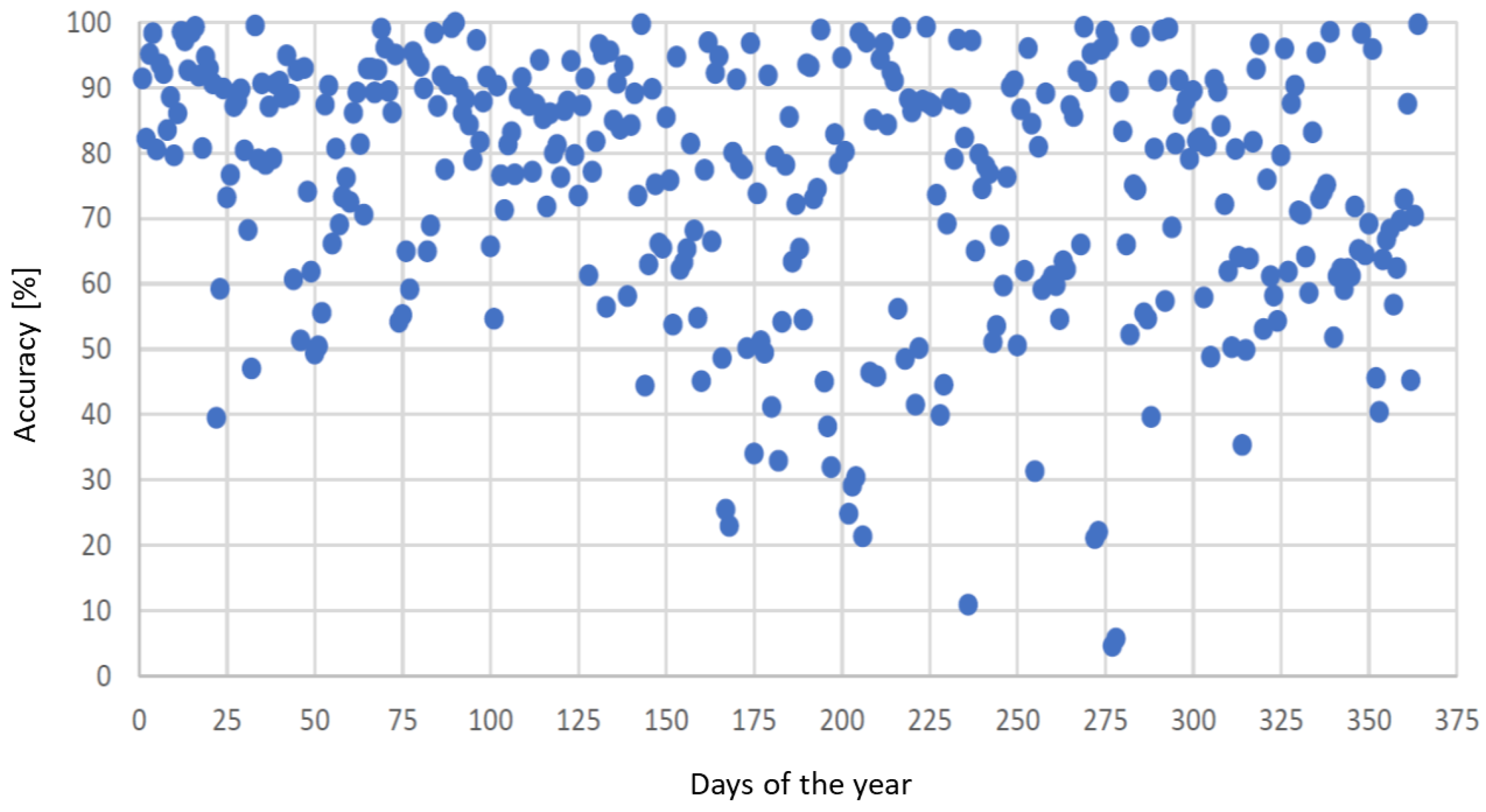
Unlike the electricity prices, which are on a rising trend, the costs of generating energy by solar installations in Germany have been dropping, with a record low of less than 5 cents/kWh in 2017 [25] (see Figure 1). Furthermore, several legislative bodies proposed reduction of taxes on electricity produced by households that is consumed on premises. This led to an increase in PV installations, reaching in 2016, a global installed capacity of 300 GWp (e.g., 45 GWp in Germany) [26].

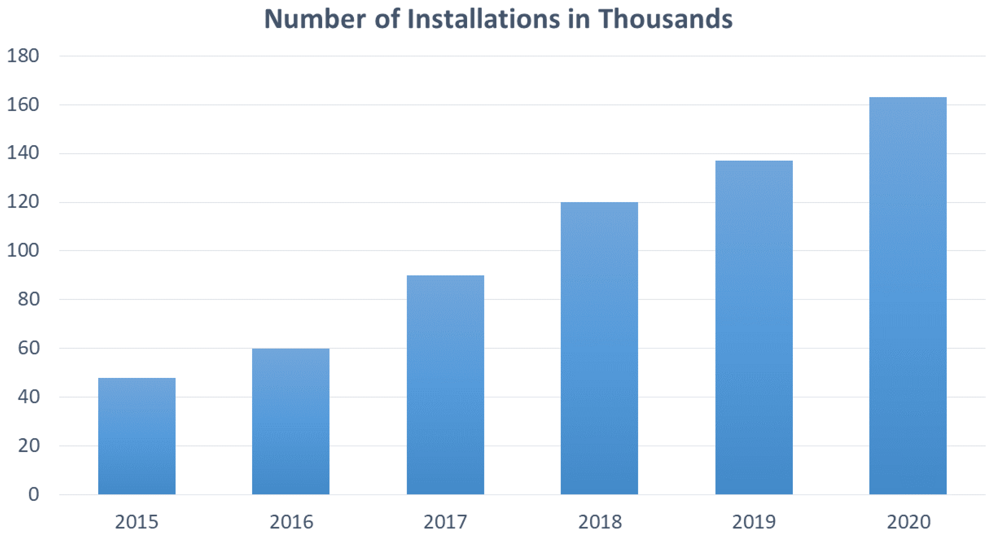
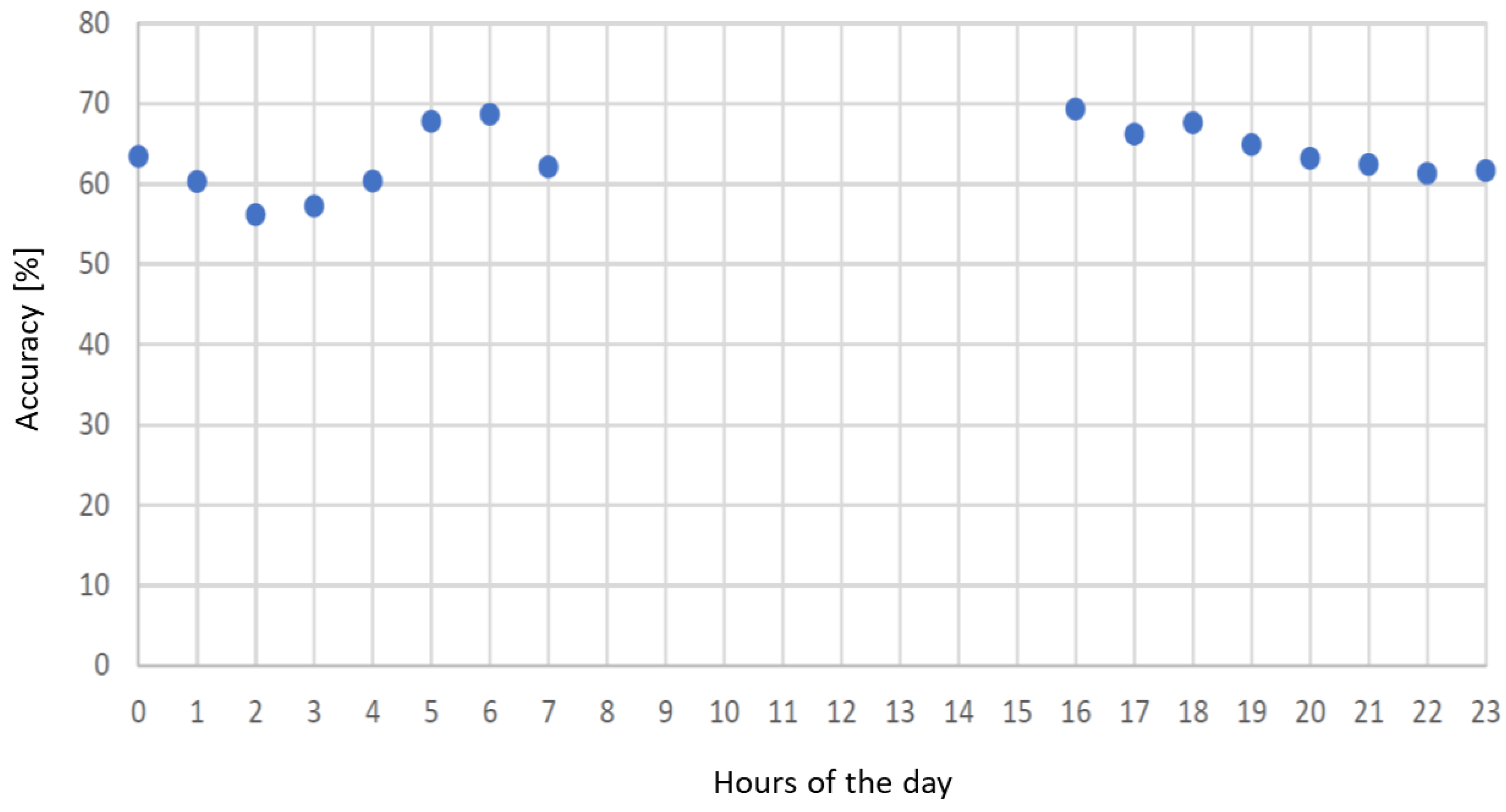
As the renewable energy sources are intermittent, and for the case of PV installations, they have an almost-zero production during certain periods of a day (e.g., 17:00 till 07:00), energy storage systems became a necessity for a better and efficient usage of the whole system. Consequently, as illustrated in Figure 2, the installation of PV-battery systems increased in Germany, with this number expected to reach an annual installations of over 20,000 systems by 2020.

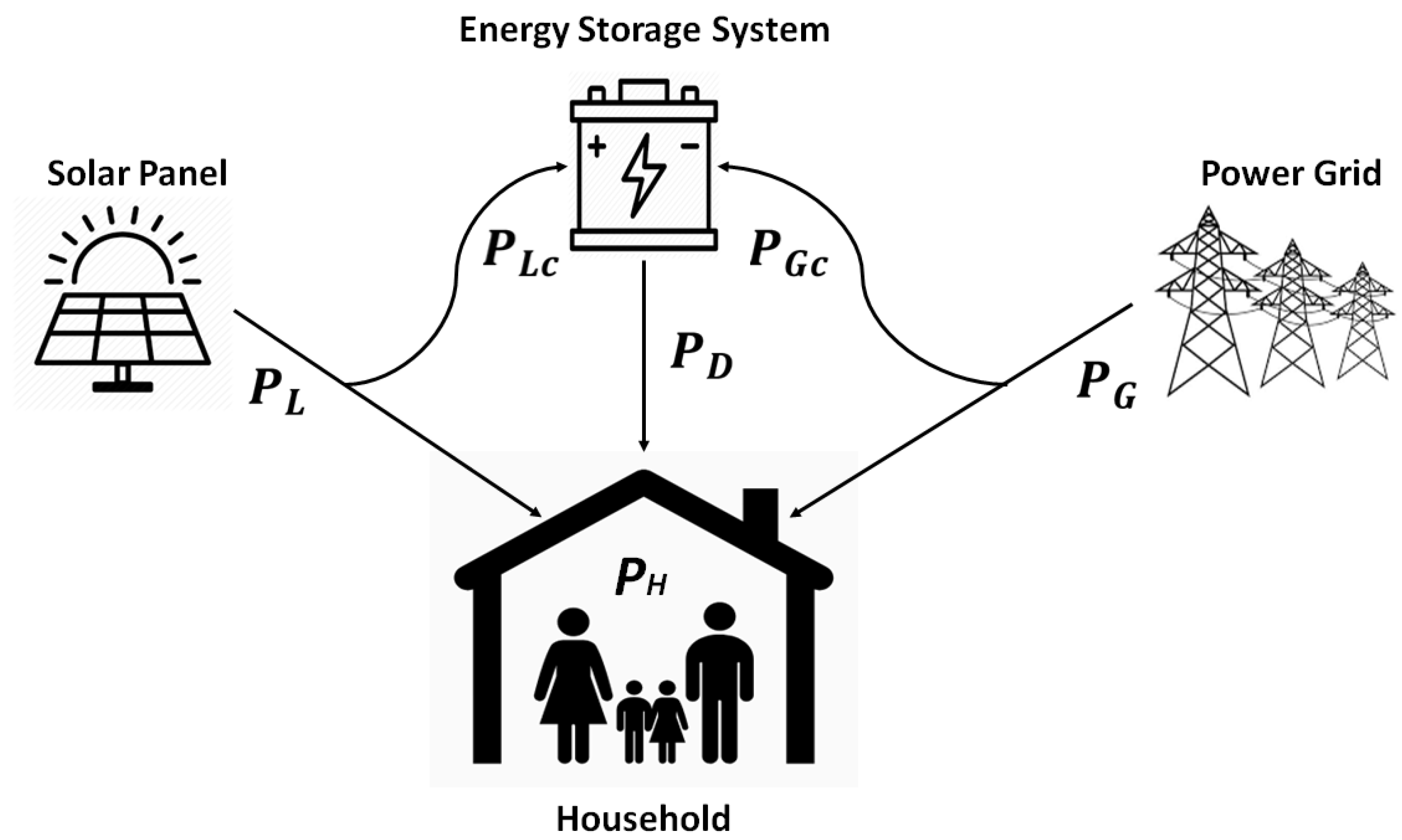
Figure 3 illustrates the underlying system for households equipped with PV-battery systems. Traditionally, the installed PV-battery system is operated in the following manner: The primary objective is always to satisfy the demand of the household (e.g., appliances). This can be achieved either through the PV generation or by drawing electricity from the grid. In the former situation, in the case that there is still a surplus of electricity generated from PV, then the battery of the system is charged (if needed). In the latter situation, the battery is charged (if needed) myopically without taking the price factor into account.

3.2. Research Question

Taking into account the system described in Section 3.1, the main research question that we are targeting in this paper is the following:

• By using locally generated electricity, would it be possible to reduce the electricity prices of a given household through intelligent energy management?

To tackle the above-mentioned research question, in this paper, unlike the current state-of-the-art myopic charging process of EV-battery systems, the electricity prices are considered the main optimization criteria based on the real-time pricing scheme (RTP). In this context, the battery is charged during cheap periods and discharged during peak (expensive) times of the day. To devise such an optimization algorithm, it requires a detailed modeling of the underlying system, which is presented next.

3.3. System Model

Figure 4 models the system under study and illustrates the corresponding power flows based on the description given in Section 3.1. For our modeling purposes, we consider discrete slots k which abstract a specific time unit (e.g., minutes, hours, days, months, years). Let $P_L\left(k\right)$ and $P_G\left(k\right)$ denote the power (kW) generated by the PV panel and drawn from the grid at time slot k respectively. Then $P_{L_c}\left(k\right)$ and $P_{G_c}\left(k\right)$ give the amount of power (kW) used from the PV panel and grid to charge the energy storage system (ESS) at time slot k respectively. We use $P_H\left(k\right)$ to present the total power demand (kW) of the household at time slot k and $e\left(k\right)$ to denote the price for households of drawing electricity from the power grid at time slot k.

Let B denote the total capacity (kWh) of the battery, whereas MD and MC present ESS’s maximum discharge and charge fractions. We use ${\alpha }_c$ and ${\alpha }_d$ to denote the charging and discharging rate limits (kW/kWh) per unit of storage respectively, with ${\mathsf{\eta }}_c$ and ${\mathsf{\eta }}_d$ being the charge and discharge efficiency both having a value of $\le 1$. Let $P_C\left(k\right)$ and $P_D\left(k\right)$ represent respectively, the power (kW) used to charge and withdraw from ESS at time slot k. Finally, we use E(k) to indicate the energy (kWh) content of the ESS at time slot k, K to present the set of time slots, and $T_u$ to denote the time slot duration (hours).

3.3.1. Constraints

The system described in Section 3.1 and modeled in Section 3.3 needs to be operated without violating certain constraints. From ESS perspective, the following constraints need to be respected:

$$0\le P_D\left(k\right)\le B\ast {\alpha }_d$$

(1)

$$0\le P_C\left(k\right)\le B\ast {\alpha }_c$$

(2)

$$E\left(k\right)=E(k-1)+{\mathsf{\eta }}_c\ast P_C\left(k\right)\ast T_u-\frac{P_D\left(k\right)}{{\mathsf{\eta }}_d}\ast T_u$$

(3)

$$MD\ast B\le E\left(k\right)\le MC\ast B.$$

(4)

As the ESS can be charged both from the local PV panel and the power grid, the following constraints need to be upheld:

$$P_C\left(k\right)=P_{L_c}\left(k\right)+P_{G_c}\left(k\right)$$

(5)

$$P_{G_c}\left(k\right)\le P_G\left(k\right)$$

(6)

$$P_{L_c}\left(k\right)\le P_L\left(k\right)).$$

(7)

The grid, local source (e.g., PV panel), and ESS have to meet the overall demand of the household, keeping in mind that some of the power from the sources is used to charge the ESS:

$$(P_L\left(k\right)-P_{L_c}\left(k\right))+(P_G\left(k\right)-P_{G_c}\left(k\right))+P_D\left(k\right)=P_H\left(k\right).$$

(8)

In Equation (8), it is very likely that the local generation by PV (e.g., $P_L\left(k\right)$) might exceed the demand of the household and needs to be curtailed. If this were to happen, the Equation (8) would be an infeasible constraint. What we want is for a new variable $P_L^{\prime }\left(k\right)$, to be the difference between the load and other sources (which are variables) while bounded by $P_L\left(k\right)$ from above and 0 from below:

$$P_L^{\prime }\left(k\right)=min\left(P_L\left(k\right),[P_H\left(k\right)+P_{G_c}\left(k\right)+P_{L_c}\left(k\right)-P_G\left(k\right)-P_D\left(k\right)){]}_{+}\right)$$

(9)

where ${\left[x\right]}_{+}$ denotes $max(0,x)$. $P_L^{\prime }\left(k\right)$ is, thus, the optimally curtailed local source, and should replace $P_L\left(k\right)$ in Equations (7) and (8).

Table 1. Definitions of the notation used (units).

Name	Description [unit]
$P_L\left(k\right)$	PV power generation in time slot k [kW]
$P_{L_c}\left(k\right)$	PV power generation used to charge the ESS in time slot k [kW]
$P_G\left(k\right)$	Power drawn from the grid in time slot k [kW]
$P_{G_c}\left(k\right)$	Power drawn from the grid used to charge the ESS in time slot k [kW]
$P_D\left(k\right)$	Power drawn from the ESS used to satisfy the demand of household in time slot k [kW]
$P_C\left(k\right)$	Power used to charge the ESS in time slot k [kW]
$P_H\left(k\right)$	Power demand of the household in time slot k [kW]
$e\left(k\right)$	Electricity price of the grid in time slot k [cent/kWh]
B	Maximum capacity of the ESS [kWh]
${\alpha }_c$ (${\alpha }_d$)	Charging (discharging) rate limit per unit of ESS [kW/kWh]
${\mathsf{\eta }}_c$ (${\mathsf{\eta }}_d$)	Charging (discharging) efficiency having a value of ≤1
$MC\left(MD\right)$	ESS maximum Charging (discharging) fraction
$T_u$	Timeslot duration [hours]
$\left|K\right|$	Number of timeslots

gives the notations and their corresponding definitions used in the above equations.

3.3.2. Objective

The objective is to minimize the electricity cost for charging the energy storage system (e.g., battery). This can be expressed mathematically over k time slots as follows:

$$\begin{array}{cc}\hfill \underset{P_L^{\prime }\left(k\right),P_{L_c}\left(k\right),P_G\left(k\right),P_{G_c}\left(k\right),P_D\left(k\right)}{min}& \sum _{k=1}^{K}e\left(k\right)\ast P_{G_c}\left(k\right)\hfill \\ \hfill \mathrm{s}.\mathrm{t}.& 0\le P_{L_c}\left(k\right),P_G\left(k\right),P_{G_c}\left(k\right)\hfill \\ \hfill & 0\le P_D\left(k\right)\le B\ast {\alpha }_d\hfill \\ \hfill & 0\le P_C\left(k\right)\le B\ast {\alpha }_c\hfill \\ \hfill & E\left(k\right)=E(k-1)+{\mathsf{\eta }}_c\ast P_C\left(k\right)\ast T_u-\frac{P_D\left(k\right)}{{\mathsf{\eta }}_d}\ast T_u\hfill \\ \hfill & MD\ast B\le E\left(k\right)\le MC\ast B\hfill \\ \hfill & P_C\left(k\right)=P_{L_c}\left(k\right)+P_{G_c}\left(k\right)\hfill \\ \hfill & P_{G_c}\left(k\right)\le P_G\left(k\right)\hfill \\ \hfill & P_{L_c}\left(k\right)\le P_L^{\prime }\left(k\right)\hfill \\ \hfill & P_L^{\prime }\left(k\right)=min\left(P_L\left(k\right),[P_H\left(k\right)+P_{G_c}\left(k\right)+P_{L_c}\left(k\right)-P_G\left(k\right)-P_D\left(k\right)){]}_{+}\right).\hfill \end{array}$$

(10)

4. Implementation

In this section, we first give, in Section 4.1, the assumptions considered for the implementation of the system described in Section 3. Based on those assumptions, we then present a cost-optimization algorithm in Section 4.2.

4.1. Considered Assumptions

It can be seen from Equation (10) that to derive a cost-optimized solution, several input parameters ($P_H\left(k\right)$, $P_{L_c}\left(k\right)$, etc.) need to be provided. Consequently, in this paper we consider certain assumptions to simplify the implementation of a cost-optimized algorithm. In this section, we present those assumptions and show the rationale behind taking them.

4.1.1. Time Slots and Duration

The objective function in Equation (10) is presented based on discrete time slots k. In this paper, we consider time slots with duration $T_u$ of 1 h (e.g., a day consists of $\left|K\right|=24$ time slots). Furthermore, we divide a given day into two modes: Light and dark. The former mode consists of time periods between 07:00 and 17:00, whereas the latter one starts at 17:00 and ends at 07:00. These distinctions are made based on the times of the day where PV panels generate power (e.g., light Mode) and have almost no generation (e.g., dark Mode).   

Dark Mode Assumption: In this paper, optimizations are considered only for the dark mode, because during this time period PV generation is almost zero. Thus, electricity needs to be drawn either from the energy storage system or from the grid. In the former case, if the state of charge of the battery is low, then the charging needs to be scheduled during cheap periods. Hence, for this mode we obtain $\left|K\right|=15$ time slots (e.g., $k=0,\dots ,14$). This is where our proposed algorithm schedules the charging of the battery optimally by minimizing, as much as possible, the charging costs.

4.1.2. Energy Consumption of Households

In order that our algorithm can schedule charging of the battery in the most cost optimal manner, it requires as an input the corresponding energy consumption of the household to which PV-battery system is installed. In our previous work of [27], a constant consumption of 500 Wh for households was considered, which was calculated by taking the average demand of the H0 profile (e.g., households) from BDEW (German Association of Energy and Water Industries). In this paper, we go one step further and analyze the energy consumption of a real household for a period of one year. Note that the methodology of this analysis is to compute the average consumption for each hour of the day by considering the corresponding hour’s energy consumption over 365 days (e.g., averaging all 365 data points at 00:00). Figure 5 illustrates the energy consumption of a typical household on an hourly-basis. It can be noticed that two peaks occur, one in the morning and another in the evening. It is worthwhile to mention that in this paper we assume no sudden demand (e.g., charging of EVs) from households. As this average household energy consumption does not reflect seasonal changes and other events happening (e.g., holidays), a more realistic energy consumption model is required. In order to prevent any complex demand profile forecasting, in this paper we consider a novel and simple assumption that the energy consumption for the dark mode (see Section 4.1.1) of the current day is similar to that of the previous day. We call this "back-to-back similarity" assumption; we analyze its accuracy next.   

Back-To-Back Similarity Assumption: Figure 6 shows the result of the analysis from the consumption perspective. Note that the methodology of this analysis is to compare the overall energy consumption during the above-mentioned periods between two consecutive days. The analysis showed that in average 75% of the time the considered "back-to-back similarity" assumption holds true. After analyzing the overall energy consumption, we further investigated the energy consumption on an hourly-basis for dark mode. Note that the methodology of this analysis is to compare the hourly-based energy consumption during the above-mentioned periods between two consecutive days. Figure 7 demonstrates that in average 60–70% of the time, the “back-to-back similarity” assumption held true. Thus, we demonstrated that the considered assumption is realistic, and prevented a tedious household demand forecast modeling processes for $P_H$.

4.1.3. Electricity Prices for Households

As for any other commodity, the prices of electricity depend strongly on demand and supply conditions. Recently, with the advent of renewable energy sources, the energy mix together with the geographic location of the generation and taxation have been playing an influencing factor on pricing. For instance during the first half of 2019, households in Germany and Bulgaria had electricity prices of 30.88 cents/kWh (highest in EU) and 9.97 cents/kWh (lowest in EU) respectively [28]. As it can be seen in Figure 8, this is due to the fact that electricity prices for households bear taxes, which vary from one country to another. To cope with peak demand, several pricing schemes, such as time-of-use (ToU) [3], real-time pricing (RTP) [4], and critical-peak pricing (CPP) [5] were proposed.

Real-Time Pricing Assumption: In this paper, we assume that the electricity prices $e\left(k\right)$ for households are based on the RTP scheme, whose prices vary from minutes to hours depending on utility company. Furthermore, hourly-based prices are given by the utility company to the customer 24 h ahead of time. An open API (https://api.awattar.de/v1/marketdata) provided by the external data source of [29] is used to obtain an hourly-based rates for the next 24 h.

4.1.4. Power Generation of PVs

One of the main factors impacting on the power generation of PVs is the irradiation. To this end, numerous scientific contributions in the literature proposed to model GHI (global horizontal irradiation). In our previous work of [27], using Pearson’s correlation, we showed that there is a high correlation between (1) power generation, (2) ambient temperature, and (3) GHI. Using the two factors of temperature and GHI and neural-network methodology, we derived a model that forecasts the power generation of PVs.

Negligible PV Generation Assumption: Due to the fact that the devised cost-optimization algorithm is for the dark mode, then we assume that the power generation by PV panels is almost negligible (e.g., $P_L\left(k\right)=0$). This assumption is realistic, because as we mentioned above, power generation by PV panels is dependent on GHI and temperature. GHI has an almost zero value in the time of the day between 17:00 and 07:00 [30], and usually the ambient temperature drops as well during that period of the day.

4.2. Heuristics-Based Cost Optimization Algorithm

Algorithm 1 presents the myopic way of charging the battery of the energy storage system without taking into account the electricity prices. In this context, the demand of the household is served from the battery (Line 5) as long as it has a state of charge more than 10% of its maximum capacity (Line 3). In case of deficit, electricity is drawn from the grid (Line 7). Whenever the battery has less than 10% of its maximum capacity, the power demand of the household is solely satisfied by the grid (Line 10); meanwhile, the battery is also charged (Lines 11 and 12).

Algorithm 1 Myopic Charging Process
Require:$E\left(0\right)$: The starting state of charge (SoC) of the energy storage system (ESS).
1:	if Dark mode then
2:	for $k=0$ to 14 do
3:	if $E\left(k\right)\ge 0.1B$ then
4:	$P_D\left(k\right)=B\ast {\alpha }_d$	// discharge the battery with the maximum discharging rate
5:	$E(k+1)=E\left(k\right)-P_H\left(k\right).T_u$	// update the state of charge of the battery
6:	if $P_D\left(k\right)<P_H\left(k\right)$ then
7:	$P_G\left(k\right)=P_H\left(k\right)-P_D\left(k\right)$	// serve the deficit demand from the grid
8:	end if
9:	else
10:	$P_G\left(k\right)=P_H\left(k\right)$	// serve the household demand from the grid
11:	$P_C\left(k\right)=B\ast {\alpha }_c$	// charge the battery with the maximum charging rate
12:	$E(k+1)=E\left(k\right)+P_C\left(k\right).T_u$	// update the state of charge of the battery
13:	end if
14:	end for
15:	end if

Algorithm 2 gives the steps for achieving a cost-optimized charging process of the battery. It can be noticed that this algorithm, by having the electricity prices for the dark mode, schedules charging the battery during cheap periods. In this context, the algorithm checks whether the battery has enough energy to satisfy the consumption of the household until the cheapest timeslot (line 6). In case it is satisfied, then the corresponding consumption is served by the energy storage system (Line 9). During cheap timeslot(s), in addition to charging the battery (Line 13), the demand of the household is satisfied by drawing electricity from the grid (Line 14). In case the battery does not have enough energy (Line 19), then electricity is drawn from the grid to charge the battery (Line 22) and to serve the demand of the household (Line 20). It is worthwhile to mention that the corresponding algorithm is a heuristic implementation of Equation (10) and does not always guarantee the optimal charging plan.

It is worthwhile to note that the main advantage of the Algorithm 2 is its ease of implementation in real-life applications use cases, which is not the case for the state-of-the-art approaches. More precisely, by taking simple but realistic assumptions, such an algorithm does not necessitate the implementation and execution of complex forecasting models (e.g., household demand) to find cost-optimized solution(s). In this respect, due to availability of limited resources (e.g., computing and storage), it is always preferable in practice to have a simplified but accurate implementation of the theory, which the Algorithm 2 achieves. Thus, we show in Section 5 that through simplified assumptions it is possible to get benefits from a real-time pricing (RTP) scheme without having to bind to feed-in tariff (FiT) schemes. Moreover, as the Algorithm 2 has no stochastic behavior, for a given input it always generates the same deterministic (i.e., not probabilistic) output. This ensures a certain quality for the obtained results and improves the time in finding the cost-optimal solution(s).

Algorithm 2 Cost-optimized Charging Process
Require:$E\left(0\right)$: The starting state of charge (SoC) of the energy storage system (ESS)     $P_H$: The set of power demand of the household such that $P_H\left(k\right)$ is an element from this set     $E_H$: The set of electricity price for the household such that $e\left(k\right)$ is an element from this set
1:	if Dark Mode then
2:	$K_{cp}$ = CheapestTimeslots($E_H$)	// set of timeslots sorted by ascending order of $e\left(k\right)$
3:	$k_{cp}$ = CheapestTimeslot($K_{cp}$)	// cheapest timeslot
4:	$C_H\left(k_{cp}\right)={\sum }_{k=0}^{k_{cp-1}}{P}_H\left(k\right).T_u$	// energy consumption of the household until the cheapest timeslot
5:	for $k=0$ to 14 do
6:	if $E\left(k\right)\ge C_H\left(k_{cp}\right)$ then
7:	if $k\ne k_{cp}$ then
8:	$P_D\left(k\right)=B\ast {\alpha }_d$	// discharge the battery with the maximum discharging rate
9:	$E(k+1)=E\left(k\right)-P_H\left(k\right).T_u$	// update the state of charge of the battery
10:	$C_H\left(k_{cp}\right)-=P_H\left(k\right).T_u$
11:	else
12:	$P_C\left(k\right)=B\ast {\alpha }_c$	// charge the battery with the maximum charging rate and cheapest price
13:	$E(k+1)=E\left(k\right)+P_C\left(k\right).T_u$	// update the state of charge of the battery
14:	$P_G\left(k\right)=P_H\left(k\right)$	// serve the household demand from the grid
15:	$K_{cp}=K_{cp}\backslash \{k_{cp}$}	// remove from the set $K_{cp}$ the cheapest timeslot $k_{cp}$
16:	$k_{cp}$ = CheapestTimeslot($K_{cp}$)	// next cheapest timeslot $k_{cp}$ such that $k_{cp}>k$
17:	$C_H\left(k_{cp}\right)={\sum }_{i=k+1}^{k_{cp-1}}{P}_H\left(i\right).T_u$	// energy consumption until the new cheapest timeslot
18:	end if
19:	else
20:	$P_G\left(k\right)=P_H\left(k\right)$	// serve the household demand from the grid
21:	$P_C\left(k\right)=B+{\alpha }_c$	// charge the battery with the maximum charging rate
22:	$E(k+1)=E\left(k\right)+P_C\left(k\right).T_u$	// update the state of charge of the battery
23:	end if
24:	end for
25:	end if

5. Evaluation of Results

In this section, we first describe the set up configuration on which Algorithms 1 and 2 were evaluated, introduce three scenarios, and then present the results.

5.1. Configuration and Scenarios

To demonstrate the benefits of the cost-optimized charging algorithm (see Algorithm 2) with respect to the myopic charging one (see Algorithm 1), we considered a real-life testbed at Fenecon GmbH. Such a testbed contained all the physical components of the system under study, as illustrated in Figure 3. A customized and open source energy management system (EMS), which is a software implementation and can be found in [31], was used in order to orchestrate in taking the adequate decisions.

In general, an EMS has the objective (based on implemented algorithms) of deciding which sources (e.g., PV generation and battery of the ESS or the grid) are used to satisfy the needs of the household. Thus, by default, the considered EMS includes the implementation of Algorithm 1 for deciding when to charge the battery of the ESS myopically. To this end, we integrated the proposed cost-optimized algorithm (see Algorithm 2) as a separate software module inside the EMS of Fenecon.

We considered during the execution of Algorithm 2, all the assumptions mentioned in Section 4.1: “back-to-back similarity” for the energy consumption of households, a “real time pricing” scheme for electricity prices, “dark Mode” for time slots, and negligible PV generation during “dark mode.” It is worthwhile to mention that the battery of the ESS has a maximum capacity B of 12 kWh and has discharging ${\alpha }_d$ and charging ${\alpha }_c$ rates of 0.75 ${\mathrm{h}}^{-1}$ (e.g., maximum discharging $P_D$ and charging $P_C$ power of 9 kW) with a charging ${\mathsf{\eta }}_c$ and discharging ${\mathsf{\eta }}_d$ efficiency of 0.93. In this paper, we do not consider the possibility of feeding-in power back to the grid (e.g., from PV or ESS). Thus the main objective was to increase self-consumption and minimize as much as possible, the electricity drawn from the grid. Consequently, the PV-battery system was analyzed from a single household perspective.

For the purpose of our evaluations, in this paper we considered the following three scenarios:

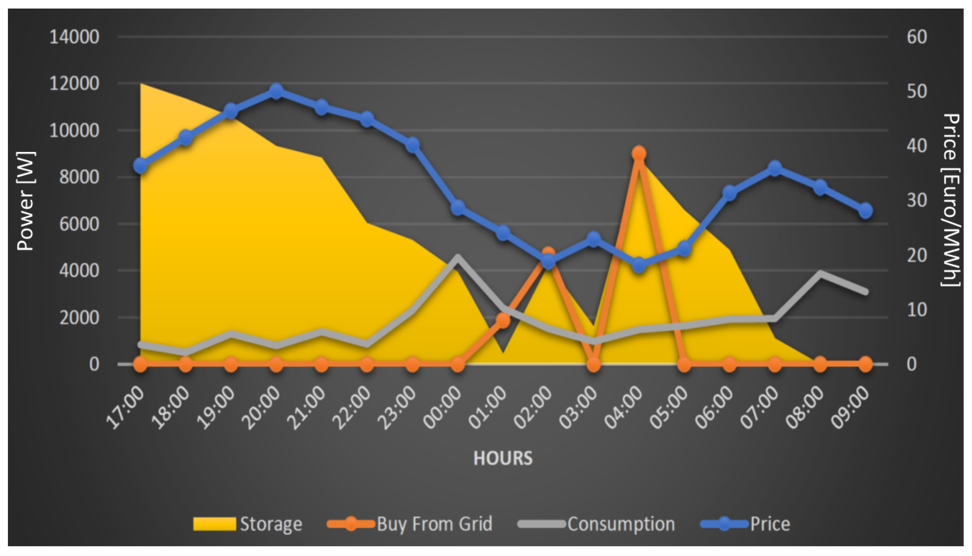
• Scenario 1: Battery is fully charged (e.g., SoC of 100%); a peak demand of the household at around 00:00; high electricity prices between 17:00 and 1100; and low prices between 00:00 and 05:00.
• Scenario 2: Battery is fully charged (e.g., SoC of 100%); two peak demands of household at around 01:00 and 06:00 respectively; high electricity prices between 17:00 and 00:00; and medium and almost flat prices between 00:00 and 07:00.
• Scenario 3: Battery is almost depleted (e.g., SoC of 20%); two peak demands of household at around 21:00 and 05:00 respectively; high electricity prices between 17:00 and 00:00; medium and almost flat prices between 00:00 and 05:00; and again, high prices between 06:00 and 07:00.

Note that for Scenario 1 and 2, the battery is fully charged in case of sunny days, whereas for cloudy days this is represented in Scenario 3. Regarding the demand of the household, Scenarios 1 and 3 represent a typically weekday, whereas Scenario 2 is for weekends.

5.2. Results

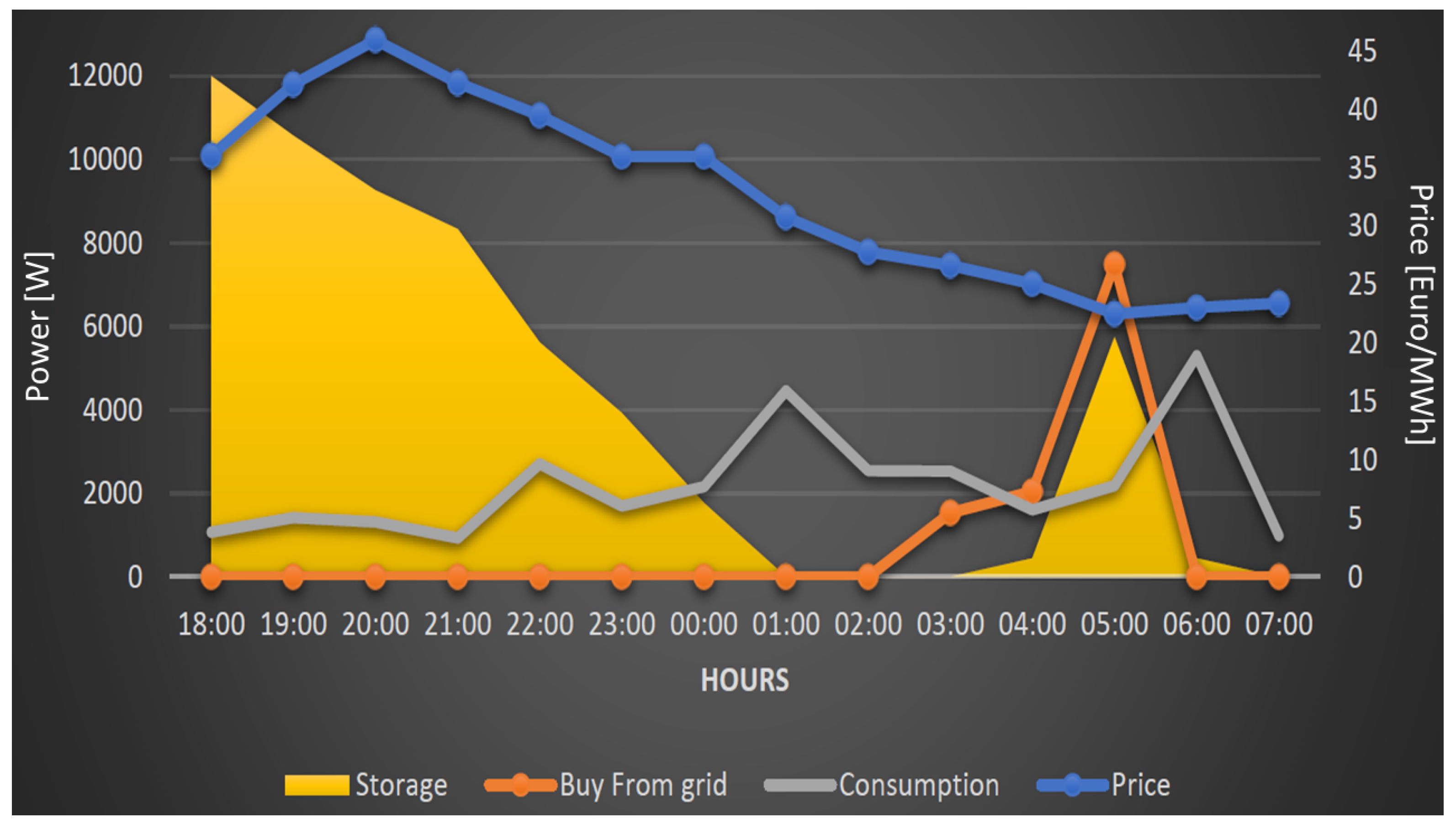
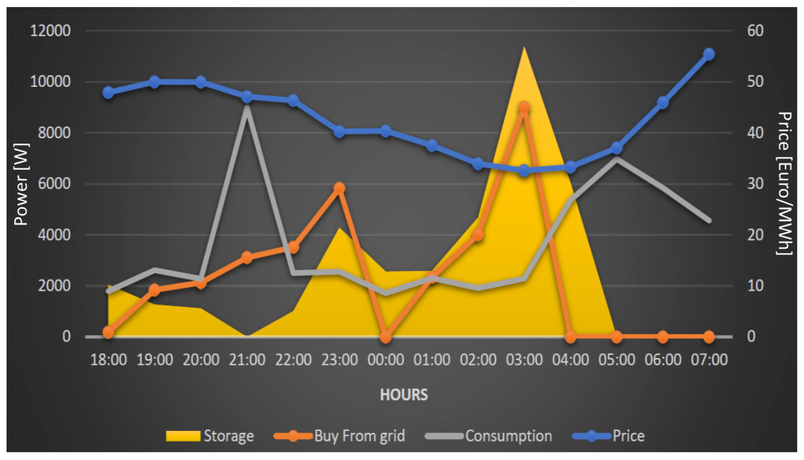
Figure 9, Figure 10 and Figure 11 illustrate the impacts of Algorithm 2 on Scenarios 1, 2, and 3 respectively. In three of those figures, the c-axis denotes the dark mode periods of the day (e.g., 17:00 till 07:00), whereas the y-axis to the left gives the power (in Watts), and to the right shows the electricity prices (in Euro per MWh). Furthermore, the yellow area illustrates the state of charge of the battery; the blue and gray lines indicate, respectively, the electricity price and power demand of the household, which through integration the total energy consumption, can be obtained. The orange line indicates the amount and the time slot when electricity is drawn (e.g., bought) from the grid.

5.2.1. Scenario 1

We can observe that Algorithm 2 plans the charging of the battery during the cheapest time slot (e.g., in this case at 02:00). As the battery of the ESS is full, together with the fact that no unexpected peak demand from household is foreseen, these allow the corresponding demand to be served by the ESS without drawing power from the grid (e.g., orange line is 0 between 17:00 and 00:00). Electricity is drawn from the grid only when the battery of ESS needs to be charged and/or the demand of the household must be satisfied (e.g., between 00:00 and 3 A.M and 4 A.M and 05:00.). It is to be noted that since at 16:00 the electricity price is second lowest after the one at 2 p.m., this algorithm (Line 16 in Algorithm 2) plans to continue charging the battery at 16:00 instead of at 15:00 (notice that no electricity is drawn from the grid at 15:00).

In

Table 2. Price comparison between different approaches for Scenario 1.

Approach	Electricity Price Paid [Euro]
Without ESS	0.7748
With ESS and myopic charging	0.5919
With ESS and cost-optimized charging	0.3234

, we compare the cost-optimized charging with respect to myopic charging and to the case where no energy storage system is installed. It can be clearly noticed that Algorithm 2 caused 50% savings with respect to the one of myopic charging and 60% cost reduction compared to the case where no ESS is installed.

5.2.2. Scenario 2

Like the previous scenario, we can observe for this one too that the Algorithm 2 plans charging of the battery during the cheapest time slot (e.g., in this case at 05:00.). Due to the fact that the battery at the beginning of the dark mode has a full capacity, it can be used to serve the demand of the household until 02:00 Consequently, during this time period, no electricity was drawn from the grid (e.g., orange line is 0 between 17:00 and 02:00). Electricity was drawn from the grid only when the battery of ESS needed to be charged (e.g., 17:00) and/or the demand of the household needed to be satisfied (e.g., between 06:00 and 06:00). It is to be noted that although the prices at 06:00 and 07:00 are relatively low, the algorithm relies on the fact that the battery will be gradually charged thanks to the PV power generated during the day.

In

Table 3. Price comparison between different approaches for Scenario 2.

Approach	Electricity Price Paid [Euro]
Without ESS	0.9226
With ESS and myopic charging	0.6675
With ESS and cost-optimized charging	0.4410

, we compare the cost-optimized charging with respect to myopic charging and to the case where no energy storage system is installed. For this scenario, Algorithm 2 caused 33% savings with respect to the one of myopic charging modes and 52% cost reduction compared to the case where no ESS is installed.

5.2.3. Scenario 3

In this scenario, as the battery at the beginning of the dark mode is almost depleted (e.g., SoC about 20% at 17:00), electricity is drawn from the grid between 17:00 and 00:00 to charge the battery and at the same time to satisfy the needs of the household. Note that this is due to the fact that the large peak of demand that happens at 21:00. As the cheapest time slot is at 03:00, Algorithm 2 plans the charging of the battery during this time slot. It is worthwhile to mention that during 00:00 and 01:00 and 04:00 and 07:00, as the battery has enough capacity to serve the demand of household, no electricity is drawn from the grid (e.g., orange line is 0 during those time periods).

In

Table 4. Price comparison between different approaches for Scenario 3.

Approach	Electricity Price Paid [Euro]
Without ESS	2.2254
With ESS and myopic charging	2.0374
With ESS and cost-optimized charging	1.9865

, we compare the cost-optimized charging with respect to myopic charging and to the case where no energy storage system is installed. It is obvious that for this scenario as the battery does not have enough capacity to serve the household during expensive periods of the day, no drastic cost savings can be achieved compared to the myopic charging processes of the ESS. However, as the cost of electricity for the case without ESS is still higher than those with ESS, then PV-battery system has still a benefit.

5.3. Discussion

From the results presented in Section 5.2, it can be noticed that electricity costs can be reduced only through the installation of the energy storage system. This allows one to exploit certain level of flexibility, especially with respect to when to charge and discharge the battery. In this respect, on the one hand, the maximum cost reduction happens for the cases (1) when the battery is full (e.g., thanks to the solar energy), and (2) electricity prices vary significantly between late night and early morning hours (see results of Scenarios 1 and 2). On the other hand, overall electricity costs reductions are less prominent when the battery is almost depleted (see the results of Scenario 3). However, in the worse case it is guaranteed to have the same electricity costs as for the case without ESS.

6. Conclusions

One of the fundamental goals of “Energy Transition” is the replacement of traditional fossil-based power generation by green and clean renewable energy sources. To circumvent the intermittency of renewables, energy storage soon became a necessity. In this respect, PV panels are being bundled together with batteries more and more in the contexts of households and commercial buildings.

In this paper, due to the technological and economical feasibility of PV-battery systems, we studied such systems by considering real-time pricing scheme. More precisely, after describing and modeling mathematical the system under study, we formulated an optimization problem. Based on this formulation, we derived a heuristics-based cost-optimization algorithm that schedules the charging of the battery during cheap time slots. To evaluate the amount of savings, we configured a testbed and considered three different scenarios, and compared them with respect to (1) no ESS being installed, (2) ESS with myopic charging, and (3) ESS with cost-optimized charging. The obtained results demonstrate that our proposed heuristics-based algorithm achieved savings with respect to the other two approaches.

As for future work, we will build on the results obtained in this paper and investigate minimizing both the curtailment and the charging cost at the same time as the main optimization criteria.