Article

A Two-Hops State-Aware Routing Strategy Based on Deep Reinforcement Learning for LEO Satellite Networks

School of Electronic Engineering, Beijing University of Posts and Telecommunications, Beijing 100876, China
*
Author to whom correspondence should be addressed.
Electronics 2019, 8(9), 920; https://doi.org/10.3390/electronics8090920
Submission received: 15 July 2019 / Revised: 18 August 2019 / Accepted: 20 August 2019 / Published: 22 August 2019
(This article belongs to the Section Microwave and Wireless Communications)

Abstract

:
Low Earth Orbit (LEO) satellite networks can provide complete connectivity and worldwide data transmission capability for the internet of things. However, arbitrary flow arrival and uneven traffic load among areas bring about unbalanced traffic distribution over the LEO constellation. Therefore, the routing strategy in LEO networks should have the ability to adjust routing paths based on changes in network status adaptively. In this paper, we propose a Two-Hops State-Aware Routing Strategy Based on Deep Reinforcement Learning (DRL-THSA) for LEO satellite networks. In this strategy, each node only needs to obtain the link state within the range of two-hop neighbors, and the optimal next-hop node can be output. The link state is divided into three levels, and the traffic forwarding strategy for each level is proposed, which allows DRL-THSA to cope with link outage or congestion. The Double-Deep Q Network (DDQN) is proposed in DRL-THSA to figure out the optional next hop by inputting the two-hops link states. The DDQN is analyzed from three aspects: model setting, training process and running process. The effectiveness of DRL-THSA, in terms of end-to-end delay, throughput, and packet drop rate, is verified via a set of simulations using the Network Simulator 3 (NS3).

1. Introduction

As the powerful supplement of terrestrial networks, the satellite networks are playing an increasingly significant role in the next generation global communication system [1]. Satellite networks inherently offer many advantages, such as worldwide coverage and better multicast ability. Compared with geostationary earth orbit (GEO) and medium earth orbit (MEO), low earth orbit (LEO) satellites system has a shorter delay, low propagation, and globally seamless coverage [2,3]. However, since LEO satellite networks are usually composed of tens or hundreds of satellites, its routing problem is more complicated than terrestrial network mainly due to its features, such as dynamic link states and unbalanced traffic load caused by arbitrary flow arrival and communication hot spots [4]. Therefore, merely applying terrestrial routing algorithm on satellite networks is impracticable.
Applied to transmit service data in the LEO satellite networks efficiently, an effective routing strategy is essential. Previously, many proposed routing strategies for LEO satellite networks focused on how to minimize end-to-end propagation delay. With the explosive growth of satellite applications, however, there are two defects shown in traditional satellite routing strategy: the packet drop rate at network layer becomes abnormally high, and the cumulative queuing delay during transmission gets non-negligibly large. An ant colony optimization-based routing strategy is proposed in [5] for LEO networks, it can adjust the routing path when the network topology changes, but requires a long convergence time. Load balance is an effective strategy to avoid congestion [6,7,8]. To guarantee a better distribution of traffic among satellites, an explicit load balancing (ELB) scheme is proposed in [9]. In ELB, the total load of the satellite is monitored. When it becomes congested, the satellite will send a notification to its neighbors and request them to decrease the sending rate. However, a part of link congestion still cannot be prevented because the ELB did not consider individual queues. To adjust the route dynamically, Song [10] set up traffic lights for each direction and proposed a public waiting queue strategy to reduce packet drop rate in [9]. However, the traffic lights routing (TLR) required global state information to calculate the best routes for each source and destination pair periodically. It may cost a lot to collect global state information due to propagation delay between satellites. Therefore, the route calculated cannot be absolutely real-time. Considering the link state may frequently change in the partial area, a state-aware and load-balanced routing (SALB) model for dynamic LEO satellite networks is proposed in [11]. However, SPT algorithm has a lack of observation of satellite networks topology. An extreme learning machine (ELM)-based distributed routing strategy is proposed in [12] for LEO networks; it can forecast the traffic at each satellite node. The simulation results show that the method in [12] has lower end-to-end delay and packet loss rate than [5]. However, the mobile agents are needed to make the routing decision in [12], which makes it difficult to track changes in network status in a timely manner.
To cope with routing packets efficiently and dynamically, a method to observe LEO satellite networks topology is necessary. Deep reinforcement learning (DRL) is valuable for establishing network models [13,14]. The authors in [15] proposed a Reinforcement Learning (RL) agent that can form an optimal policy through a series of trial-and-error processes with its environment. The RL-based routing in [16] is adaptive to link changes by choosing a next-hop node based on various local states. In [17], Deep Learning (DL) was guaranteed to be efficient for characterizing the appropriate input and output pattern in a highly dynamic network. Combining RL with DL, a Double-Deep Q Network (DDQN) is proposed in [18], which is more excellent for handling a large number of states than Q-Learning, and solved the problem of overestimating Q function value in traditional DQN.
In this paper, we analyze the link status of the LEO satellite network. We use the deep learning method to enable satellite nodes to learn the link status within two hops. Therefore, each satellite node can make the next hop selection autonomously according to the link status. Our main contributions in this paper are summarized as follows.
  • A two-hops state-aware routing strategy based on deep reinforcement learning (DRL-THSA) is proposed for LEO satellite networks. In DRL-THSA, each node collects link state information within two-hop neighbors and makes routing decisions based on the information. The link state information is interacted between nodes through Hello packets; therefore, the DRL-THSA discover the node failure event in time and change the next hop node.
  • A setup and update method of link state is proposed. The link state is divided into three levels, and the traffic forwarding strategy for each level is presented, which allows DRL-THSA to cope with link congestion.
  • The routing decision method based on the DDQN network is proposed, and the DDQN is analyzed from three aspects: model setting, training process and running process.
The remainder of this paper has the following structure: In Section 2, the LEO satellite networks model, which includes the satellite networks topology, setup and update of link state, and two-hops state aware updating, are described. In Section 3, the deep reinforcement learning model setting and routing algorithm are presented in detail. The experimental results are discussed in Section 4, and Section 5 draws the conclusions.

2. LEO Satellite Networks Model

At the beginning of this section, we first explain the definition of the symbols used later in Table 1.

2.1. Satellite Networks Topology

The LEO system is modeled as a direct graph G = ( V , E ) , where V represents the set of satellites and E represents the set of inter-satellite links (ISLs). Each satellite has four ISLs, including two intra-plane ISLs and two inter-plane ISLs [
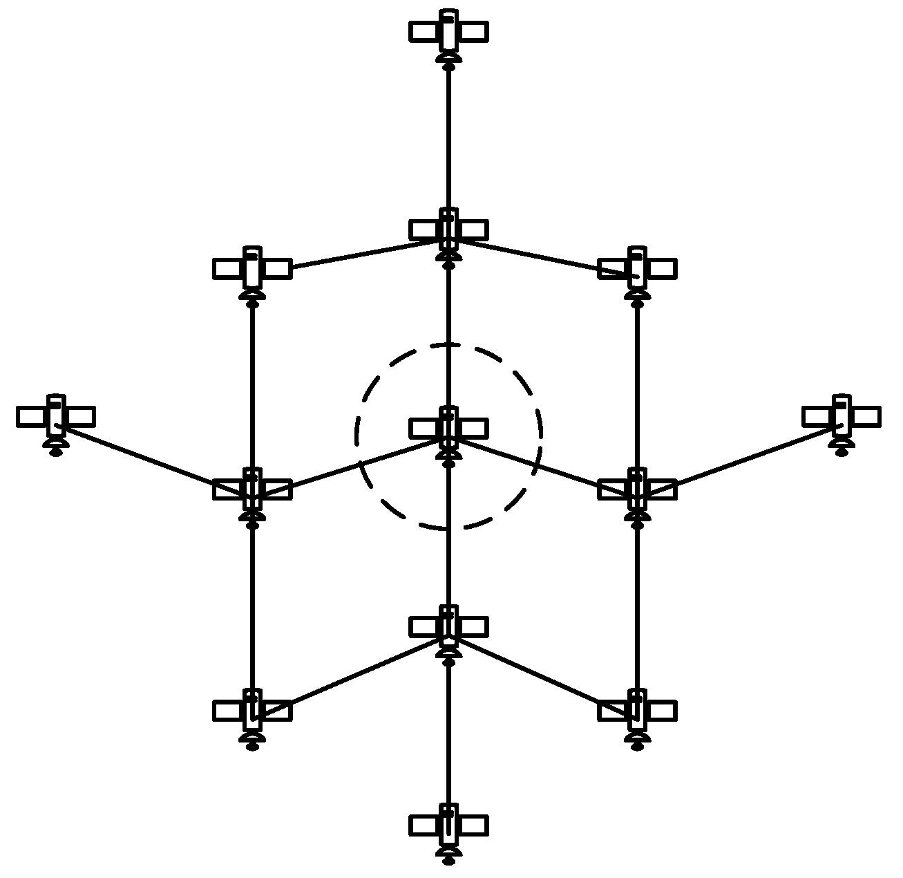
19]. Due to the extreme variation of the angular velocity of inter-plane ISLs—the ISLs within cross-seam—the north and south pole area cannot be built. As to simplify the change of network topology, we adopt the Virtual Node (VN) strategy to set up a satellite networks topology. In VN-based topology, a virtual node is supposed to be the current physical satellite, which is above the specific surface of the earth [20]. A virtual node and a physical satellite correspond one to one at any time, and the correspondence will change if a physical satellite moves out of the coverage of current VN or into the coverage of another VN [
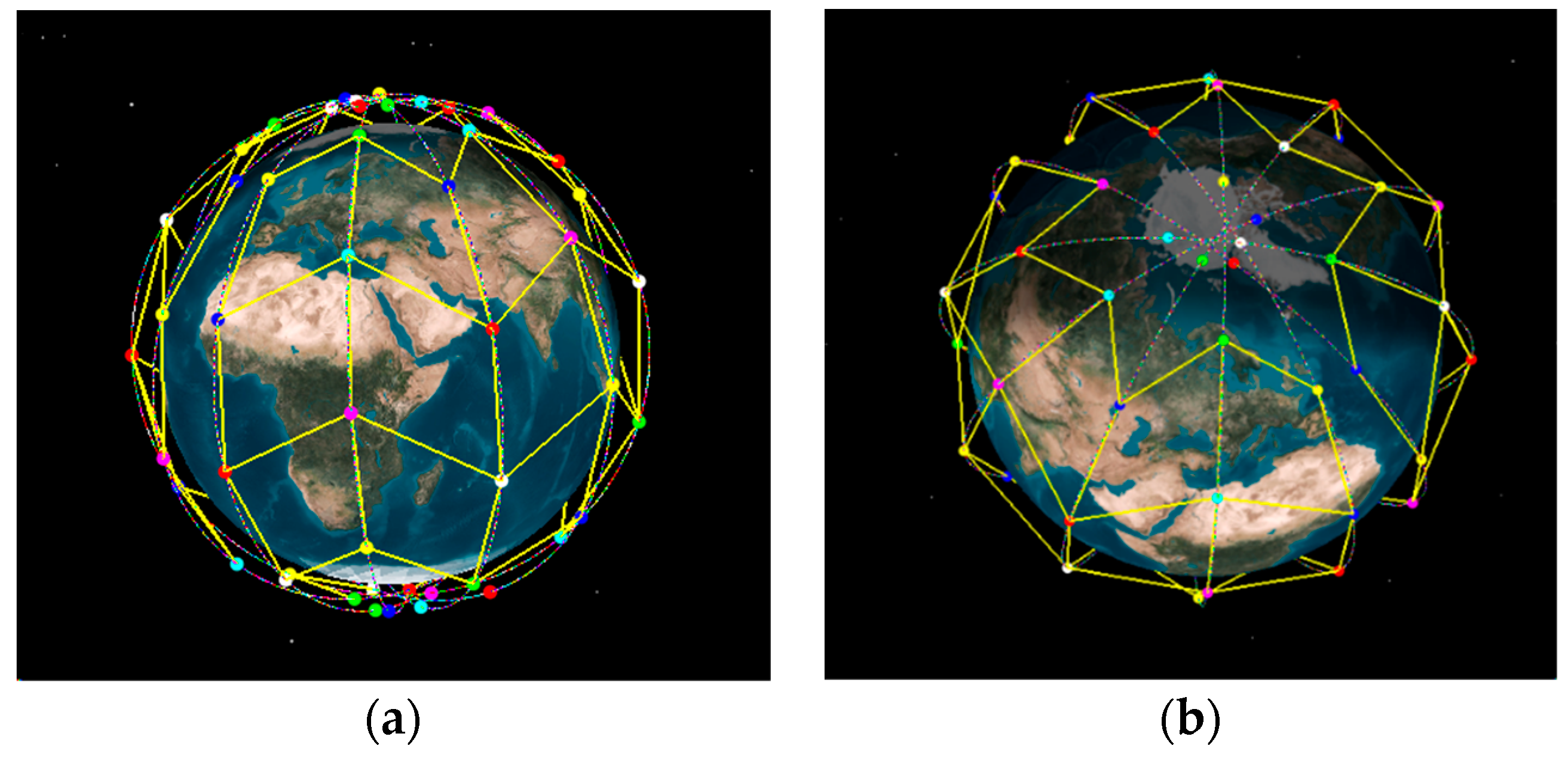
21]. The process of correspondence changing is called handoff. When a handoff happens, the state information will be transferred from the former physical satellite to the latter. In this way, rotating physical satellites can be converted into fixed virtual nodes, and the dynamic topology is also transformed into an accordingly static one. As it is shown in Figure 1, we construct the LEO satellite networks based on STK.

2.2. Setup and Update of Link State

In satellite networks, when satellite receives a packet, the packet is inserted into the buffer queue at one direction by sequence, waiting to be sent out. However, the buffer space is limited, and accumulated packets will fill up the whole queue if the traffic is too heavy. Then the packets which still get into the queue will be dropped. Therefore, it is essential to monitor the queue to reduce unnecessary packets loss.
Let t c denote the queue check interval, according to the average input packet rate I a v g ( t t c ) and the average output packet rate O a v g ( t t c ) in the past, and we predict the average input packet rate I a v g and the average output packet rate O a v g in the next t c seconds with Equations (1) and (2):
I a v g = ( 1 λ I ) I a v g ( t t c ) + λ I I a v g ( t )
O a v g = ( 1 λ O ) O a v g ( t t c ) + λ O O a v g ( t )
where λ I and λ O represent the weight of the past average input rate and the past average output rate, respectively, 0 < λ I < 1 , 0 < λ O < 1 . These weights act as filters. The average input packet rate and the average output packet rate are desired to represent the long average packet rate, which should be counted over a long period. The short-term light traffic load needs to be filtered. Therefore, the selection of λ I and λ O are essential. If these weights are too large, the average packet rate will nearly equal the instantaneous traffic load. Otherwise, if these weights are too small, it is hard for the average packet rate to represent the long-range traffic load, which results in ineffective estimation and routing computation. In this paper, the values of λ I and λ O are assigned dynamically according to the traffic load by Equations (3) and (4).
λ I = { max { I a v g ( t ) I a v g ( t t c ) α 1 , a 0 } , I a v g ( t ) < I a v g ( t t c ) min { I a v g ( t ) I a v g ( t t c ) I a v g ( t t c ) , α 2 }                                e l s e
λ O = { max { O a v g ( t ) O a v g ( t t c ) α 1 , a 0 } , O a v g ( t ) < O a v g ( t t c ) min { O a v g ( t ) O a v g ( t t c ) O a v g ( t t c ) , α 2 }                                e l s e
Thus, the estimated average rate does not change much when the instantaneous traffic load is closed to the estimated traffic load in the last interval. The short-term light traffic load is filtered, and the average packet rate can be estimated effectively.
In DRL-THSA, for a given direction, L max denotes the max length of the buffer queue, and L ( t ) represents the current length of the buffer queue. Therefore, the queue occupancy rate is calculated by Equation (5).
q = L ( t ) L max [ 0 , 1 ]
To avoid dropping a packet, it is crucial to make sure that the queue is not full before the next check. The predicted queue occupancy rate is calculated by Equation (6).
p = q + [ I a v g O a v g ] t c L max
In this way, two cases can be envisioned:
  • p 1 : It means packet drop may happen in the next t c seconds. Therefore, the link state is set to be congested whatever the current queue occupancy rate is. The threshold T 1 and T 2 should meet T 1 = T 2 = 0 .
  • p < 1 : The thresholds should be adjusted to fit the average input packet rate I a v g and the average output packet rate O a v g . The threshold T 1 and T 2 meet
    ( T 2 T 1 ) L max = [ I a v g O a v g ] t c
    ( 1 T 2 ) L max = [ I a v g O a v g ] t c
Considering the extreme situation, we get
T 1 = min ( max ( 1 2 [ I a v g O a v g ] t c L max , 0 ) , 1 )
T 2 = min ( max ( 1 [ I a v g O a v g ] t c L max , 0 ) , 1 )
The link state is marked as Free State (FS) when q is below T1 and is considered to be Busy State (BS) if q is between T 1 and T 2 . It is defined as Congested State (CS) when q exceeds T 2 .
To monitor and control the load effectively, if the link state is BS or CS, the satellite should send a notification including the traffic reduction ratio X to its neighbor and request it to decrease the input packet rate to I a v g X .
When the satellite enters BS, assuming the desired time for a satellite to reside in FS is set to be t s , the traffic reduction ratio is calculated by Equations (11) and (12).
T 2 = min ( max ( 1 [ I a v g O a v g ] t c L max , 0 ) , 1 )
X = min ( max ( I s I a v g , 0 ) , 1 )
When the satellite enters CS, it should require its neighbor to stop transmitting the packet immediately. Therefore, X is set to be 0.

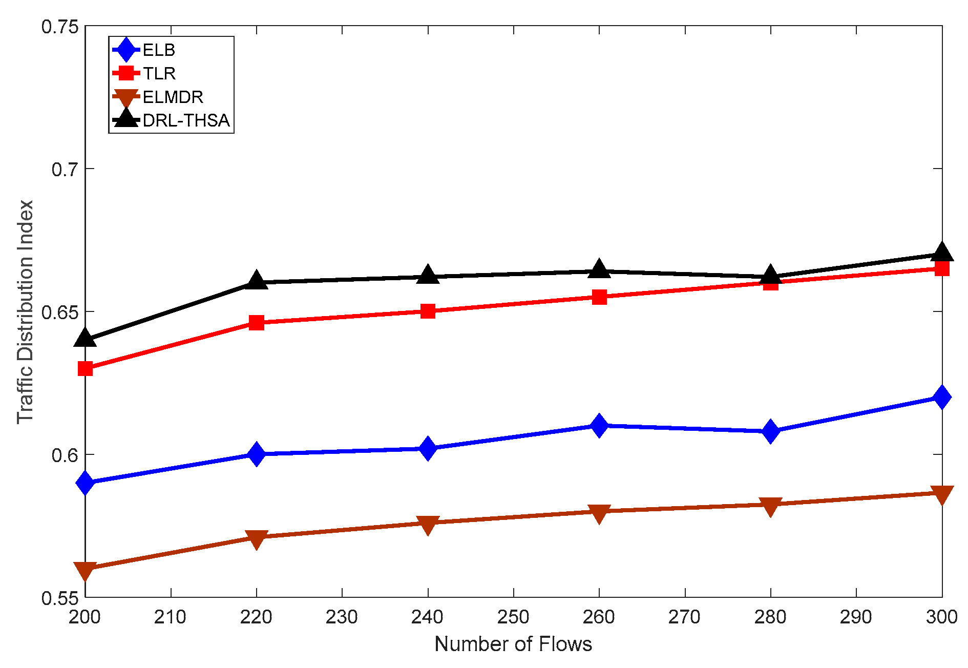
2.3. Two-Hops State Aware Updating

Taking a given satellite as the center, two-hops states consist of the link states of all the ISLs within two-hops. It is shown in Figure 2.
In DRL-THSA, each satellite keeps both link state table (LST) and neighbors’ link state tables (NLST). The link states are stored as the style in Table 2.
To monitor the link connectedness, we adopt the HELLO packet strategy proposed in the open shortest path first routing scheme [22]. The satellite sends HELLO packets to its neighbors with the period t h The connectedness is defined to be off if the current satellite does not receive the acknowledgment (ACK) message from the direction n within t d . It may not change states until it receives the HELLO packets periodically. When the change happens, the current satellite updates its LST and broadcasts the connectedness change messages to all the other neighbors.
To monitor the link state, satellites check the buffer queue of all the directions with the period t c . If the current link state is different from the previous one, the current satellite will update its LST and send the link state change messages to its neighbor satellites.
When satellite receives the message from neighbors, it updates NLST according to the information contained in the message. The process of dynamic two-hops state aware updating is shown in Algorithm 1.
Algorithm 1 Dynamic Two-Hops State Aware Updating
Connectedness Updating:
while true do
  broadcast HELLO packets
  wait t h
end while
if receive ACK within t d then
  if ( t is up to date) then
    LST( N , n ).connectedness ← On
  else
    drop the message
  end if
else
  LST( N , n ).connectedness ← Off
end if
Link State Updating:
while true do
  calculate T 1 and T 2
  evaluate link state
  LST( N , n ).state← s t a t e
  wait tc
end while
Neighbor Link State Updating:
Receive link change message
if ( t is up to date) then
  continue
else
  drop the message
end if
if (NLST( N , n ).state is not equal to s t a t e ) then
  NLST( N , n ).state← s t a t e
else
  drop the message
end if

3. Routing Strategy Based on Deep Reinforcement Learning

3.1. Deep Reinforcement Learning Model Setting

The satellite networks topology was converted into a 2D plan, shown in Figure 3. Reinforcement learning observes the information obtained in the satellite networks topology, which functions as the environment.
In deep reinforcement learning, an agent is modeled as a four-tuple consisting of { S , A , P , R } , where S is a set of states, A is a set of actions. P is the state transition probability that represents the probability of a switch from one state to another state, and R is a reward function that represents a reward r received from the operating environment. Combining the deep reinforcement learning with satellite routing strategy, we construct the model { S , A , P , R } as Table 3.
where [ N s , N d , L S T ] represents routing source node, destination node, and current satellite’s LST. N n e x t represents the decision of next-hop satellite node. P is set to be P n e x t calculated by Equation (13):
P n e x t = ( i = 1 , 2 , , m s i ) 1
where m represents the number of neighbors for current satellite node, and s i represents the number of link states of neighbor satellite i .
When the packet is routed from N s to N d , the reward r is calculated by Equations (14) and (15):
d i f ( N s , N d ) = α ( R A A N s R A A N d ) 2 + β min [ | ω s ω d | 2 , ( 2 π | ω s ω d | ) 2 ]
r = { r d r c d i f ( N s , N d )     N n e x t = N d N n e x t   f a i l e d / c o n g e s t e d O t h e r
where R A A N represents right ascension of ascending node. ω represents the mean anomaly. α and β are the weights of inter-plane ISLs and intra-plane ISLs. We define r d as a high reward for success and r c as a punishment for mistake.

3.2. Routing Algorithm

The DDQN model observes the information of the satellite networks topology through the training process. However, the training process of DDQN requires a large amount of overhead, and it takes a long time. Due to limited resources and processing capacity on the satellite, we simulate the flows of the satellite networks and complete the DDQN training process on the ground. The off-line training process enables the DDQN model to cope with all the link states that may be encountered. Then the trained DDQN models are stored on the satellite and no longer updated during the satellite routing process.

3.2.1. Double-DQN Offline Training Process

Double-DQN uses Deep Neural Networks (DNN) instead of the look-up table to represent all the states and actions. The inputs of the DNN are the current states, and the outputs are the Q-values of all the possible actions. We propose to use the DDQN which is composed of an online DNN with weight θ o n l i n e and a target DNN with weights θ t arg e t . DNN needs to be trained to achieve convergence state. The online DNN updates its weights θ o n l i n e at each iteration. The target DNN resets its weights θ t arg e t to θ o n l i n e in every N t arg e t iterations and keeps weights θ t arg e t fixed at other iterations. The loss function at the current iteration is shown in Equation (16):
L D D Q N = Ε [ Y D D Q N Q ( s , a , θ o n l i n e ) 2 ]
where the target value Y D D Q N is defined as
Y D D Q N = r + γ Q ( s , arg max Q i ( s , a ; θ o n l i n e ) ; θ t arg e t a A )
To minimize the loss function, it needs to update the weights θ by using the experience < s , a , r , s > to train the DNN. The DDQN can execute action a by the ε -greedy policy to balance its exploration and exploitation. Algorithm 2 shows the DDQN train algorithm which uses the DDQN to find the optional routing policy.
Algorithm 2 Double-DQN train algorithm
Input: A ; N t arg e t ; N b ; M
Output: DDQN routing model
Initialize: θ o n l i n e ; θ t arg e t
for episode i = { 1 , , N } do
  for iteration t = { 1 , , T } do
    Execute action a according to ε -greedy policy
    Receive reward r t
    Store experience < s , a , r t , s > in M
    if an episode terminates at iteration j + 1 then
      Set Y j D D Q N = r d
    else
      Determine a = arg max a A Q ( s , a ; θ o n l i n e )
      Set Y j D D Q N = r j + γ Q ( s , a ; θ t arg e t )
    end if
      Perform a gradient descent step on L D D Q N to update θ o n l i n e
      Reset θ t arg e t = θ o n l i n e in every N t arg e t iterations
  end for
end for
Accordingly, based on the experience e , the online DNN computes the optional value Q ( s , a ; θ t arg e t ) . Then, the loss function L D D Q N and the target value Y D D Q N are calculated according to Equations (14) and (15) respectively. The value of L D D Q N is used to update weights θ o n l i n e . To make sure the stability of the learning, DDQN uses the experience reply memory M to store experience e , and a mini-batch of N b experiences are taken at each iteration to train the DNNs. Because the network topology environment changes with the destination node. For the whole LEO satellite networks, the number of DDQN is equal to the number of satellites.

3.2.2. Double-DQN On-Board Running Process

The trained DDQN models are attached to the satellite. During the DDQN on-board running process, each satellite calculates the optimal next hop by inputting the two-hops link states to the corresponding DDQN model, and then the next hop node repeats the process until the packets arrive at the destination. In addition, DRL-THSA considers a total of four cases in LEO satellite networks including link failure, link recovery, link state change, and endless-loop route. The routing strategy can competently cope with the dynamic changes of the satellite networks by effectively handling these cases, observing the two-hops state information and training the DDQN. Algorithm 3 shows the workflow of DRL-THSA routing strategy.
Algorithm 3 Workflow of DRL-THSA
1: Update the threshold T 1 and T 2 at whole directions of current satellite node N c
2: Evaluate link states and update LST
3: if link state changes then
     Broadcast LST to neighbors
   end if
4: Updating neighbor link state (NLST) by receiving link states information from neighbors
5: Load DDQN according to destination node N d
6: Input [ N c , N d , L S T ] to DDQN
7: Output the next-hop satellite N n e x t
8: Input [ N n e x t , N d , N L S T ] to DDQN
9: Output the two-hops satellite N t w o
10: if N t w o is equal to N c then
     Suppose L S T ( N n ) . c o n n e c t edness to be Off temporarily
     Go to step 6;
   else
     continue
  end if
11: transmit the packet to satellite node
  • Link ( N , n ) failure: Current satellite has not received ACK message from the direction n within t d . It is defined as link ( N , n ) failure. Then it should update L S T ( N , n ) . s t a t e . When the routing task is coming, it is required to input the latest link state to DDQN.
  • Link ( N , n ) recovery: When current satellite received ACK message from node n periodically, it is defined as link ( N , n ) recovery. Then it needs to update L S T ( N , n ) . s t a t e . When the routing task is coming, it is required to input the latest link state to DDQN.
  • Link ( N , n ) state change: The link states are divided into three cases according to the thresholds T 1 and T 2 . When the link state changes from low load state to high load state, such as from FS to BS and from BS to CS, the current satellite will update L S T ( N , n ) . s t a t e , then send the link state change message and transmission rate reducing message. In contrast, if the link state changes from high load state to a low one, satellite updates L S T ( N , n ) . s t a t e and sends the link state change message only.
  • Endless-loop route: This will cause a serious packet drop problem. Combining two-hops state aware with the observation of DDQN is the key to avoid endless-loop route. According to the calculation by DDQN, if the N t w o is equal to N c , it means endless-loop occurs. We suppose the link connectedness of the current next-hop satellite N n e x t to be off during this routing process. Repeat the routing strategy until the N t w o is not equal to N c . Then the N n e x t is chosen to transmit the packet.
Traditional calculation strategies such as Dijkstra require too much computation resources because of global routing table updating. In fact, there may be only one link state change. DRL-THSA makes full use of the two-hops link state information which is partially updated. It significantly reduces the updating overhead when only a few link states change. However, it is not applicable to the networks where the number of disconnected links is destructive. In addition, there is no need for DRL-THSA to recalculate when link states change owing to the fact that DDQN has known how to route them in the whole cases.

4. Simulation and Results

4.1. Parameters Setup

To evaluate the proposed DRL-THSA, we use NS-3.29 (Network Simulator 3, Version 3.29) as the simulation tool to construct the simulations in an Iridium-like satellite network with 66 satellites distributed over six planes. Except for the satellites along the seam where cross-seam ISLs cannot be built, each satellite maintains two inter-plane ISLs and two intra-plane ISLs. Intra-plane ISLs keep connected all the time while inter-plane ISLs only work outside the polar area [23]. The capacity of ISLs is set to 25Mbps. The average packet size is set to 1 KB and the queue length is set to 100 packets. We utilize 200 On–Off flows and the On–Off period of each flow follows a Pareto distribution with the shape of 1.5. The average burst and idle time are both set to 500ms. Traffic load can be controlled by adjusting the data transmission rate of sources or the number of flows. The main system parameters are shown in Table 4. According to the experience, the greedy value of ε is set as 0.9. All the simulations are run for 60s equivalent to that in [9]. All scenarios are run 100 times, and the average values are considered as the final results.
We evaluate our routing model, the ELB [9], the TLR [10] and the Extreme Learning Machine-based distributed routing (ELMDR) [12] under the same scenario for the comparison from three aspects: average end-to-end delay, packet drop rate, and system throughput.

4.2. Results

4.2.1. End-to-End Delay

The total delay of packets that arrived at their destination is recorded. To measure the performance of DRL-THSA under different traffic conditions, different individual data transmission rate and number of flows are used in the simulation. When the individual data transmission rate varies from 2.5 Mbps to 3.5 Mbps, the number of flows is fixed to 200. The purpose is to evaluate the system performance when the number of flows is unchanged and the transmission rate is changed. When the number of flows increases from 200 to 300, the individual data transmission rate is fixed to 3.5 Mbps. The purpose is to evaluate the system performance when the transmission rate is unchanged and the number of flows changes. The average end-to-end delay for different transmission rates is shown in Figure 4. The average end-to-end delay for different number of flows is shown in Figure 5.
It can be seen that the average end-to-end delay of DRL-THSA is smaller than that of ELB, TLR and ELMDR. The reason is that the DRL-THSA filters out the impact of short-term light traffic load while counting the average input rate and the output rate. The ELMDR needs to discover the routing path and pass back to the source node through the mobile agent. Therefore, when the transmission rate increases, the link state during the routing path may change from the idle state to the congestion state, so that the end-to-end delay of the data packet increases. Since the TLR and ELB do not consider the impact of short-term light traffic fluctuations on routing computation, the short-term light traffic load will lead the TLR and the ELB to choose this link. Therefore, the packets might be sent to the short-term light traffic load nodes and increase the congestion level, which brings a longer average end-to-end delay. Another reason is that the DRL-THSA alternates path according to route state within two-hops, which avoids more queuing delay. The routing strategy is determined by the DDQN model, which is per-training. The more accurate estimation of the average traffic rate, the more accurate the state entered into the DDQN, which provides a more optimal route than TLR and ELB. In Figure 5, the average end-to-end delay of DRL-THSA increases with the increasing of flows. Since the congestion of node is tried to be avoided, the packets will be transmitted on another routing path, which increases the average end-to-end delay.

4.2.2. Packet Drop Rate

The performance of DRL-THSA is evaluated by the total packets drop rate. The total packets are recorded to obtain the drop rate. Figure 6 and Figure 7 show the total packet drop rate with different transmission rates and different number of flows. It should be noted that the links between satellites are assumed as error-free. Thus, the packets are dropped when the queue buffer of the satellite is not enough. In other words, the satellite has been congested. Furthermore, when the time to live (TTL) of a packet decreases to zero, this packet is dropped. It can be seen that the packet drop rate of DRL-THSA is lower than that of the ELB, TLR and ELMDR. According to the routing mechanism, ELMDR has the highest packets drop rate. The reason is that the pass back routing information of ELMDR under high traffic load may be outdated. At the same time, the packets drop rate of ELB is higher than that of the TLR. The reason is that the congestion at the current hop is not considered in the ELB. Therefore, packets might be dropped before sending. In DRL-THSA, the DDQN considers the node state within two-hops and routes the packets through the optimal path. Thus, the DRL-THSA can be seen as a dynamic optimal routing strategy which can avoid the congestion before it occurs. The TLR only considers the node state within one hop, and the congestion might be occurring at the next hop when the next hop cannot find a suitable node to route the packets. In Figure 7, the packets drop rate increases with the increasing of the number of flows. The reason is that since more packets are routed to the sub-optimal next hop, the TTL of packets is more likely to decrease to zero.

4.2.3. System Throughput

Figure 8 and Figure 9 show that the DRL-THSA has the highest throughput among the three routing strategies. It should be noted that the traffic load has been balanced among all the satellites in DRL-THSA strategy, resulting in higher throughput than that of ELB, TLR and ELMDR.

4.2.4. Traffic Distribution Index

The traffic distribution index in [10] is used to investigate how well the traffic is distributed over the entire constellation, which can be expressed as
I n d e x = ( i = 1 n x i ) 2 n i = 1 n x i 2
where n is the number of ISLs and x i represents the actual number of packets that traversed the i t h ISL. The higher the value of the traffic distribution index is, the better the traffic is distributed over the entire constellation. Figure 10 and Figure 11 show the traffic distribution index performance of these three routing strategies. It can be seen that the DRL-THSA outperforms the ELB, the TLR and the ELMDR.
In order to verify that DRL-THSA can alleviate congestion and reduce queueing delays, the average queue occupancy of each satellite is shown in Figure 12. The simulations are performed for cases where the individual data transmission rate is fixed to 3.5Mbps and the number of flows is fixed to 300. It can be seen that the DRL-THSA obtains the lowest average queue occupancy, which means that congestion is alleviated throughout the network. There are two reasons for DRL-THSA traffic with a more uniform traffic distribution than ELB, TLR and ELMDR. The first reason is that the DRL-THSA filters the shore-term light traffic load. The second reason is that the ε -greedy value of DDQN is set as 0.9. Therefore, DRL-THSA has a chance to explore the next-hop node autonomously, thus further diverting the traffic flow.

5. Conclusions

In this paper, a Two-Hops State-Aware Routing Strategy Based on Deep Reinforcement Learning (DRL-THSA) for LEO satellite networks is presented. In DRL-THSA, we propose a mechanism to evaluate link states for adjusting the dynamic traffic in satellite networks and put forward a two-hops state-aware strategy to update the real-time link states. When the link states changes, it may broadcast the changes to its neighbors for updating the LST. To observe the information contained in LEO satellite networks topology, we train DDQN models through a simulated routing environment. According to the training efficiency and the convergence degree of the network, the ε -greedy value of DDQN is chosen as 0.9. Combined with the two-hops state-aware strategy, our models can figure out the optimal next hop for routing packets, and they can also handle situations including link failure, link recovery, link state change, and endless-loop route. Simulation results demonstrate that DRL-THSA performs well in terms of end-to-end delay, throughput, and packet drop rate and traffic distribution index. In future research, we will study the impact of deep learning network structure and parameter settings on routing strategy performance.

Author Contributions

C.W. proposed the basic framework of the research scenario. In addition, C.W. was in charge of modeling the problem and proposed the routing strategy. H.W. did the simulations and wrote the paper. W.W. gave some suggestions on the mathematical model and formula derivation.

Funding

This work was supported by the National Natural Science Foundation of China (NSFC) under the Grant No. 61801033.

Conflicts of Interest

The authors declare no conflict of interest.

References

  1. Qu, Z.; Zhang, G.; Cao, H.; Xie, J. LEO Satellite Constellation for Internet of Things. IEEE Access 2017, 5, 18391–18401. [Google Scholar] [CrossRef]
  2. Guo, Q.; Gu, R.; Dong, T.; Yin, J.; Liu, Z.H.; Bai, L.; Ji, Y.F. SDN-based end-to-end fragment-aware routing for elastic data flows in LEO satellite-terrestrial network. IEEE Access 2018, 7, 396–410. [Google Scholar] [CrossRef]
  3. Xu, W.; Jiang, M.; Tang, F.L.; Yang, Y.Q. Network coding-based multi-path routing algorithm in two-layered satellite networks. IET Commun. 2017, 12, 2–8. [Google Scholar] [CrossRef]
  4. Liu, Z.L.; Li, J.S.; Wang, Y.R.; Li, X.; Chen, S.Z. HGL: A hybrid global-local load balancing routing scheme for the Internet of Things through satellite networks. Int. J. Distrib. Sens. Netw. 2017, 13. [Google Scholar] [CrossRef]
  5. Gao, Z.H.; Guo, Q.; Wang, P. An adaptive routing based on an improved ant colony optimization in LEO satellite networks. In Proceedings of the Sixth International Conference on Machine Learning and Cybernetics, Hong Kong, China, 12–14 November 2007; pp. 1041–1044. [Google Scholar]
  6. Li, J.; Kameda, H. Load balancing problems for multiclass jobs in distributed/parallel computer systems. IEEE Trans. Comput 1998, 47, 322–332. [Google Scholar] [CrossRef]
  7. Tang, F.L.; Guo, M.Y.; Guo, S.; Xu, C.Z. Mobility prediction based joint stable routing and channel assignment for mobile ad hoc cognitive networks. IEEE Trans. Parallel Distrib. Syst. 2016, 27, 789–802. [Google Scholar] [CrossRef]
  8. Kameda, H.; Li, J.; Kim, C.G.; Zhang, Y.B. Optimal Load Balancing in Distributed Computer Systems; Springer: London, UK, 1997. [Google Scholar]
  9. Taleb, T.; Mashimo, D.; Jamalipour, A.; Kato, N.; Nemoto, Y. Explicit load balancing technique for NGEO satellite IP networks with on-board processing capabilities. IEEE-ACM Trans. Netw. 2008, 17, 281–293. [Google Scholar] [CrossRef]
  10. Song, G.H.; Chao, M.Y.; Yang, B.W.; Zheng, Y. TLR: A traffic-light-based intelligent routing strategy for NGEO satellite IP networks. IEEE Trans. Wirel. Commun. 2014, 13, 3380–3393. [Google Scholar] [CrossRef]
  11. Li, X.; Tang, F.L.; Chen, L.; Li, J. A state-aware and load-balanced routing model for LEO satellite networks. In Proceedings of the 2017 IEEE Global Communications Conference, Singapore, 4–8 December 2017; pp. 1–6. [Google Scholar]
  12. Na, Z.Y.; Pan, Z.; Liu, X.; Deng, Z.A.; Gao, Z.H.; Guo, Q. Distributed Routing Strategy based on Machine Learning for LEO Satellite Network. Wirel. Commun. Mob. Comput. 2018, 1–10. [Google Scholar] [CrossRef]
  13. Pan, J.; Wang, X.S.; Cheng, Y.H.; Yu, Q. Multisource Transfer Double DQN Based on Actor Learning. IEEE Trans. Neural Netw. Learn. Syst. 2018, 29, 2227–2238. [Google Scholar] [CrossRef] [PubMed]
  14. Ding, R.J.; Xu, Y.D.; Gao, F.F.; Shen, X.M.; Wu, W. Deep Reinforcement Learning for Router Selection in Network with Heavy Traffic. IEEE Access 2019, 7, 37109–37120. [Google Scholar] [CrossRef]
  15. Wang, D.L.; Sun, Q.Y.; Li, Y.Y.; Liu, X.R. Optimal Energy Routing Design in Energy Internet with Multiple Energy Routing Centers Using Artificial Neural Network-Based Reinforcement Learning Method. Appl. Sci. 2019, 9, 520. [Google Scholar] [CrossRef]
  16. Al-Rawi, H.A.A.; Ng, M.A.; Yau, K.L.A. Application of reinforcement learning to routing in distributed wireless networks: A review. Artif. Intell. Rev. 2015, 43, 381–416. [Google Scholar] [CrossRef]
  17. Kato, N.; Fadlullah, Z.M.; Mao, B.M.; Tang, F.; Akashi, O.; Inoue, T.; Mizutani, K. The deep learning vision for heterogeneous network traffic control: Proposal, challenges, and future perspective. IEEE Wirel. Commun. 2016, 24, 146–153. [Google Scholar] [CrossRef]
  18. Van Hasselt, H.; Guez, A.; Silver, D. Deep reinforcement learning with double q-learning. Comput. Sci. 2015, arXiv:1509.06461. [Google Scholar]
  19. Lu, Y.; Zhao, Y.J.; Sun, F.C.; Qin, D.H. Complexity of routing in store-and-forward LEO satellite networks. IEEE Commun. Lett 2015, 20, 89–92. [Google Scholar] [CrossRef]
  20. Jia, X.H.; Lv, T.; He, F.; Huang, H.J. Collaborative data downloading by using inter-satellite links in LEO satellite networks. IEEE Trans. Wirel. Commun. 2017, 16, 1523–1532. [Google Scholar] [CrossRef]
  21. Lu, Y.; Sun, F.C.; Zhao, Y.J. Virtual topology for LEO satellite networks based on earth-fixed footprint mode. IEEE Commun. Lett. 2013, 17, 357–360. [Google Scholar] [CrossRef]
  22. Fortz, B.; Thorup, M. Internet traffic engineering by optimizing OSPF weights. In Proceedings of the 2000 IEEE Infocom, Tel Aviv, Israel, 26–30 March 2000; pp. 519–528. [Google Scholar]
  23. Tang, F.L.; Zhang, H.T.; Yang, L.T. Multipath Cooperative Routing with Efficient Acknowledgement for LEO Satellite Networks. IEEE. Trans. Mob. Comput. 2018, 18, 179–192. [Google Scholar] [CrossRef]
Figure 1. Satellite networks topology. (a) Equatorial region; (b) Polar region
Electronics 08 00920 g001
Figure 2. Inter-satellite links within two hops.
Electronics 08 00920 g002
Figure 3. Virtual Node (VN)-based satellite networks topology.
Electronics 08 00920 g003
Figure 4. The average end-to-end delay with different transmission rates.
Electronics 08 00920 g004
Figure 5. The average end-to-end delay with different number of flows.
Electronics 08 00920 g005
Figure 6. The packet drop rate with different number of rates.
Electronics 08 00920 g006
Figure 7. The packet drop rate with different number of flows.
Electronics 08 00920 g007
Figure 8. The total throughput with different sending rates.
Electronics 08 00920 g008
Figure 9. The total throughput with different number of flows.
Electronics 08 00920 g009
Figure 10. The traffic distribution index with different sending rates.
Electronics 08 00920 g010
Figure 11. The traffic distribution index with different number of flows.
Electronics 08 00920 g011
Figure 12. The average queue occupancy for each satellite.
Electronics 08 00920 g012
Table 1. Definition of the symbols.
SymbolDefinition
G The direct graph of the LEO system
V The set of satellites
E The set of inter-satellite links
t c The queue check interval
I a v g ( t ) The average input packet rate
O a v g ( t ) The average output packet rate
I a v g The prediction average input packet rate
O a v g The prediction average output packet rate
λ I The weight of the past average input rate
λ O The weight of the past average output rate
α 0 , α 1 , α 2 Parameters   to   calculate   λ I   and   λ O
L max The max length of the buffer queue
L ( t ) The current length of the buffer queue
q The queue occupancy rate
p The predicted queue occupancy rate
T 1 The threshold between free state and busy state
T2The threshold between busy state and congested state
X The traffic reduction ratio
t s The desired time for a satellite to reside in free state
N The index of satellite node
n The direction of inter-satellite link, n [ 1 , 2 , 3 , 4 ]
t The timestamp of link state
t h The period of HELLO packet
t d The maximum acknowledgment time of HELLO packet
L S T ( N , n ) Link state table of satellite N at direction n
N L S T ( N , n ) Link state table of neighbor satellite N at direction n
S The   set   of   states ,   represented   by   [ N s , N d , L S T ]
A The   set   of   actions ,   represented   by   N n e x t
P The   state   transition   probability ,   represented   by   P n e x t
R The reward, represented by r
N s The source node
N d The destination node
m The number of neighbors for current satellite node
s i The number of link states of neighbor satellite i
R A A N The right ascension of ascending node
ω The mean anomaly
α The weight of inter-plane ISL
β The weight of intra-plane ISL
r d The reward for success
r s The punishment for mistake
θ o n l i n e The weight of online DNN
θ t arg e t The weight of target DNN
Ntarget The   number   of   iterations   to   reset   θ t arg e t
ε Greedy value for DDQN
Table 2. Link state table.
NodeDirectionConnectednessLink StateTimestamp
NnOn/OffFree/Busy/Congestedt
Table 3. Agent model of reinforcement learning.
Parameters S A P R
Interpretation State ( [ N s , N d , L S T ] ) Action ( N n e x t ) Possibility ( P n e x t ) Reward (r)
Table 4. System parameter.
GeneralAltitude780 km
Polar region boundary latitude70
Routing recomputation period600 ms
ISL bandwidth25 Mb/s
Up/down bandwidth25 Mb/s
Packet length1 kB
Simulation time length60 s
DRL-THSA α 0 0.02
α 1 0.1
α 2 0.3
t c queue check interval30 ms
ISL buffer queue size100
t s the desired time for a satellite to reside in free state200 ms
t h the period of HELLO packet30 ms
t d the maximum acknowledgment time of HELLO packet30 ms
ε the greedy value for DDQN0.9
TLRISL buffer queue size75
Public waiting queue size100
Public waiting checking interval30 ms
Maximum waiting time90 ms
ELBISL buffer queue size100
ELMDR α 1
ρ 0.75
q 1 0.2
c 1 0.7
c 2 0.3

