Article

Application of L1 Trend Filtering Technology on the Current Time Domain Spectroscopy of Dielectrics

Key Laboratory of Engineering Dielectrics and Its Application, Ministry of Education, Harbin University of Science and Technology, Harbin 150080, China
*
Author to whom correspondence should be addressed.
Electronics 2019, 8(9), 1046; https://doi.org/10.3390/electronics8091046
Submission received: 15 August 2019 / Revised: 6 September 2019 / Accepted: 16 September 2019 / Published: 18 September 2019
(This article belongs to the Section Circuit and Signal Processing)

Abstract

:
The current time domain spectroscopy of dielectrics provides important information for the analysis of dielectric properties and mechanisms. However, there is always interference during the testing process, which seriously affects the analysis of the test results. Therefore, the effective filtering of current time domain spectroscopy is particularly necessary. L1 trend filtering can estimate the trend items exactly in a set of time series. It has been widely used in the fields of economics and sociology. Therefore, this paper attempts to apply L1 trend filtering to the current time domain spectroscopy. Firstly, polarization and depolarization currents are measured in the laboratory. Then the test results are filtered by L1 trend filtering and the filtering effects are compared with several common filtering algorithms, such as a sliding mean filter and Savitzky–Golay smoothing filter. Finally, the robustness and time complexity of L1 trend filtering are analyzed. The filtering results show that because the polarization currents vary in a wide range of the time domain (about 2–3 orders of magnitude), smooth and undistorted curves in the whole test time range can hardly be obtained through common filtering algorithms, while they can be obtained by L1 trend filtering. The results of robustness analysis and time complexity analysis show that L1 trend filtering can extract the trend items accurately in the time series under given different noise levels, and the execution time is also lower than 176.67 s when the number of tested points is no more than 20,000. Those results show that L1 trend filtering can be applied to the time domain current spectroscopy of dielectrics.

1. Introduction

The time domain spectrum of insulating dielectric current refers to the currents flowing through the insulating dielectrics during the application of a step voltage and short circuit, which are called polarization currents and depolarization currents, respectively. Macroscopic parameters (conductivity, dielectric constant, and loss factor) and microscopic parameters (polarizability, space charge) can be obtained by polarization and depolarization currents, and the corresponding internal microstructures can be inferred. It is an effective means to understand the physics essence of insulating dielectrics [1,2,3,4,5,6,7,8]. In recent years, most scholars have applied polarization and depolarization current to the diagnosis of insulation aging state. By equivalent the dielectric to the extended Debye model, the model parameters are solved according to the measured current results. Then the relationship between the model parameters and aging state is analyzed to judge the aging degree of insulation [9,10,11,12,13,14]. Therefore, it is very important to obtain accurate polarization and depolarization currents for dielectric properties and aging state analysis.
In the process of polarization and depolarization current testing, there is always interference, which include external space noise, test instrument noise, and output voltage fluctuation of high voltage DC power supply. Since the polarization and depolarization currents of insulating dielectrics are relatively weak (especially when the polarization and depolarization processes tend to be steady), the currents caused by interference have a large influence on the test results of polarization and depolarization currents. Therefore, it is of great significance to weaken the influence of interference on the test results of the time domain current spectrum of dielectrics.
To reduce the influence of interference, one method is to improve the hardware condition of the test system, including a shielding box with effective shielding and high-voltage DC power supply with a small ripple coefficient. Another method is using digital filtering technology to filter the measured currents. That is, to filter the sampled signal by mathematical algorithm and reduce the proportion of interference in the measured signal. In some harsh test environments, even if the hardware conditions meet the test requirements, the interference still exists in the test results. Therefore, it is necessary to take some digital filtering methods to filter the measured currents. It has the advantage of not being limited by the test conditions to weaken the influence of interference. There are many kinds of digital filtering algorithms, and each of which has its corresponding application range [15,16,17]. However, there are few reports about which filtering technology is suitable for the filtering of polarization and depolarization currents.
L1 trend filtering is an effective algorithm for estimating potential trends in signal waveforms, which is widely used in economics, finance and the social sciences [18]. This paper attempts to apply L1 trend filtering to time domain current spectrum filtering of insulating dielectrics. Firstly, the theory of L1 trend filtering technology is introduced. Then the polarization and depolarization currents are measured under laboratory conditions, and the test results are filtered by L1 trend filtering and several commonly filtering algorithms. The filtering effects of different filtering methods are compared and analyzed in detail. Finally, the robustness of L1 trend filtering method is analyzed. The research ofn the time domain current spectrum filtering of dielectrics aims to provide an important prerequisite for accurate analysis of test results, and forms an important basis for accurate acquisition of the dielectric properties of insulating dielectrics.

2. Basic Theory of L1 Trend Filtering

With the rapid development of digital signal processing technology, the estimation of the potential trend from the tested signal waveform appears in various disciplines. L1 trend filtering was first proposed by Kim et al. [19] in 2009. It is widely used in economics, geophysics, finance, social sciences, management, and biomedicine because of its advantages of fast processing speed, tracking the changing trend of unsteady signals, complexity of linear computation, and easy realization.
In L1 trend filtering, the aim is to minimize the objective function which is shown in Equation (1):
f = 1 2 t = 1 n ( y t x t ) 2 + λ t = 2 n 1 | x t 1 2 x t + x t + 1 |
where y t is the time series obtained by testing and n is the number of points. x t is the intrinsic trend series with estimation and y t x t is the fluctuation term. λ is a nonnegative parameter used to control the trade-off between smoothness of x t and the size of residual. The first part 1 2 t = 1 n ( y t x t ) 2 of Equation (1) is to measure the fluctuation component by least square function, and the second part λ t = 2 n 1 | x t 1 2 x t + x t + 1 | is to measure the smoothness degree of trend component by first-order difference calculation. The two parts are connected by regular parameter λ ( λ 0 ), which is used to adjust the proportion of two parts. When the objective function is minimum, x t which is the estimated value of trend term could be obtained. The relative solution about x t , which is estimated, has been elaborated in detail in [19]. As a result of too many details about the solution principle, in order to save space, the detailed description of the solution principle of x t is not introduced in this paper.
Equation (1) can be converted into the matrix norm form of Equation (2):
f = 1 2 y x 2 2 + λ D x 1
where y = ( y 1 , y 2 , , y n ) R n , x = ( x 1 , x 2 , , x n ) R n , and u 1 = i | u i | represents the L1 norm of the vector, and D R ( n 2 ) × n it is a second-order difference matrix:
D = [ 1 2 1 1 2 1 1 2 1 1 2 1 ]
The objective function (Equation (1)) is a strictly convex function with unique solutions. The optimization process is based on regression analysis. Since it is impossible to find the analytic solution, the filtering results in the following sections are all numerical solutions which are solved by using CVX module of the MATLAB platform. The relevant MATLAB procedures is added in the Appendix A.

3. Test of the Current Time Domain Spectrum

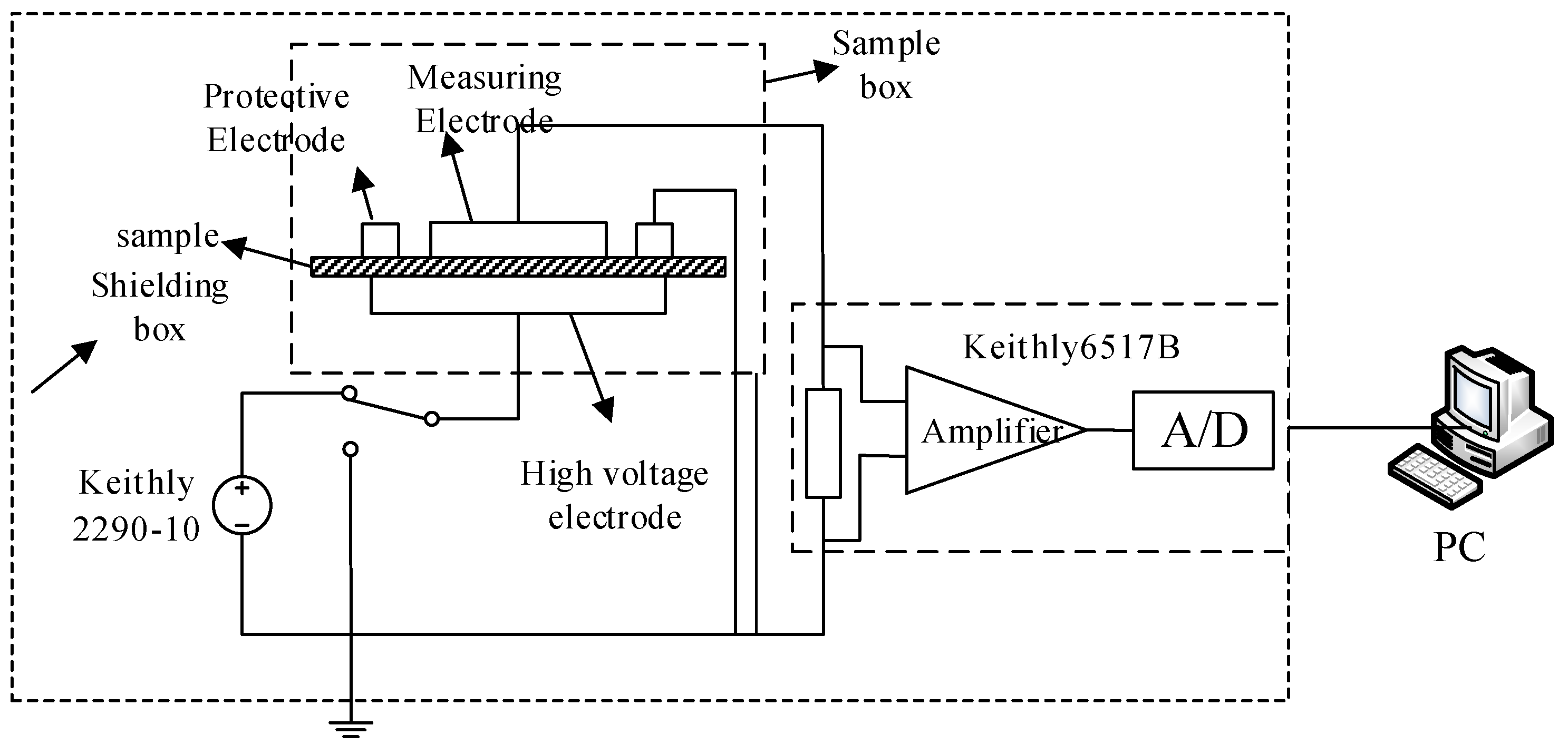
3.1. The System of Measurement of the Current Time Domain Spectrum

To study the filtering technology of polarization and depolarization currents, it is necessary to establish a system to test the polarization and depolarization currents of insulating dielectrics. In this paper, a polarization and depolarization current testing system is established in the laboratory. The hardware consists of a Keithly 2290-10 (Tektronix, Beaverton, OR, USA) high-voltage DC power supply (maximum output voltage is 10 kV), a Keithly 6517B (Tektronix, Beaverton, OR, USA) electrometer (measurement accuracy is 1 femto ampere.), shielding box, sample box, and computer. For software, the test program is written and a man-machine interface is established through LabVIEW (National Instruments, Austin, TX, USA). The information about the amplitude of test voltage and acquisition time is set on the control panel of the program to realize the automatic reading, recording, and saving of currents. The currents are recorded once a second during the test process, and the test time of polarization and depolarization currents is 7200 seconds. The block diagram of the measurement system is shown in Figure 1.

3.2. Test Results of the Current Time Domain Spectrum

The polarization and depolarization currents of 20% SiC/PE composites under different electric field strength were measured. The results of polarization and depolarization currents under the electric field strength of 30 kV/mm were given here, as shown in Figure 2. Since the polarization and depolarization currents vary in a wide range (about 2–3 orders of magnitude) over the whole range of test time. If the polarization and depolarization currents are plotted in linear coordinates, the variation of current in the later stage of measurement cannot be seen. Therefore, to better observe the variation of currents with time during the whole testing process, the polarization and depolarization currents are always plotted in a logarithmic scale [1,2,9,10].
As shown in Figure 2, in the whole test time domain, the polarization and depolarization currents are influenced by the interference to different degrees. In the initial stage of applying the voltage and short circuit, the influence of the interference on the measured currents is relatively small, due to the larger value of the measured currents. In the later stage of applying the voltage and short circuit, the value of measured currents is very small and greatly affected by the interference. Therefore, it is necessary to filter the polarization and depolarization currents, especially for the currents during the later stage. In addition, due to the interference of DC high voltage source, the fluctuation in steady state of the polarization currents is much larger than that in the depolarization currents. Therefore, when the filtering method is effective for the polarization currents, it is also effective for the depolarization currents. The filtering results in the following chapters are analyzed with polarization currents as an example. In addition, due to the lager value of the first few points, the effects of interference on the first few filtered points are very little, which can be ignored. Therefore, in this paper, there is little concern about the filtering effects of the first few points. The major concerns is filtering effects of tested points in the later stage of test process, excluding the first few test points, such as the first five or ten test points.

4. Filtering Results and Analysis

4.1. The Filtering Results with L1 Trend Filtering Algorithms

Since this is the first time that a L1 trend filter has been applied to the time domain spectrum of the polarization currents, there is no reference to determine the reasonable range of the regularization parameter λ. To obtain the optimal filtering effects, it is necessary to change the parameter λ by several orders of magnitude, and then to select the effective range of parameter λ according to the corresponding filtering results. Therefore, the regularization parameter λ are selected as 10, 100, 1000, 10,000, and 100,000, respectively. The filtering results of different values of λ are shown in Figure 3a.
Figure 3a shows that the L1 trend filtering effect is very poor when λ = 10 and λ = 100, and there is still great interference in the later stage of the polarization currents after filtering. With the increase of the λ value, the polarization current curve after filtering becomes smoother. However, when λ equals 100,000, the filtering results will be distorted at the beginning of a period of time. Through the filtering results of Figure 3a, the reasonable range of λ can be determined between 1000 and 100,000. To further understand the influence of parameter λ on the filtering effects, six λ values in the range of 1000–100,000 are selected to filter the polarization currents. The filtering results are shown in Figure 3b. At the same time, in order to analyze the filtering effects more clearly, the filtering results when λ equals 10,000 are presented separately, as shown in Figure 3c.
As shown in Figure 3b, when the range of variation of the λ value (1600–24,000) is within an order of magnitude, the influence of different λ on the filtering results is little for the overall trend. With the increase of the value of λ, the last segment of the filter curves of the polarization currents are smoother. From Figure 3c, it can be seen that the curve obtained by L1 trend filtering with λ = 10,000 is not distorted and is very smooth in the whole test time range.

4.2. Filtering Results with Several Common Filtering Algorithms

The commonly used smoothing filtering methods include sliding average filtering, Savitzky–Golay smoothing filtering and wavelet filtering. Due to the limitation of space, the principles of filtering algorithms are not introduced. The filtering effects of different filtering algorithm are only analyzed.

4.2.1. Filtering Results with Sliding Mean Filtering

The selection of the number of adjacent data m in the moving average method will directly influence the filtering effects of the test data. To observe the influence of different m values on the filtering results clearly, the values of parameter m are selected to 10 and 1000, respectively. The filtering effects are shown in Figure 4.
According to Figure 4, when m = 10, the sliding mean filter has good filtering effects on the initial stage of the polarization currents, but poor filtering effects on the last stage of the polarization currents. When m = 1000, the current filtering curve is very smooth at the whole test time, but the filter results of the initial stage are much larger than the test results, leading to the obvious distortion. There is an obvious discontinuity at a time of 500 s. According to the filtering results with m = 10 and m = 1000, it can be inferred that with the increase of m, the better the filtering effect is, but the more serious the distortion of the polarization current is in the initial stage. In addition, for the period of time the beginning and the ending, because the number of the measured data used to calculating the average value is less than m (the closer to the two endpoints, the less the number of measured data used), the filtering results are not very accurate, which affects the accurate analysis of the steady-state polarization currents. Taking m = 1000 as an example, the distortion is obviously in the last stage of the polarization currents marked with the green rectangle.

4.2.2. Filtering Results with Savitzky–Golay

In the Savitzky–Golay smoothing method, the amount of data in the filtering window (window width) m and the number of polynomials p used for fitting will affect the smoothing effect of the data. In this paper, the number of polynomials p is taken as 2, and the width of the filtering window m is 40 and 400, respectively. The filtering results are shown in Figure 5.
According to Figure 5, when m = 40, Savitzky–Golay filter has good filtering effects on the initial stage of the polarization currents, but it has poor filtering effects for the polarization currents after a period of time (after 2000 s, approximately). When m = 400, the current filtering curve is very smooth in the whole test time, but the filtering curves in the initial stage of the polarization current are obviously distorted. Due to m = 400, there are obvious discontinuities at a time of 200 s, which are similar to the problems existing in the sliding mean filter mentioned above.

4.2.3. Filtering Results with Wavelet Transform

Wavelet decomposition layer J in wavelet transform filtering is one of the factors affecting the effects of the wavelet transform. The larger the decomposition layer J is, the better the separation of the signal and noise. However, if the decomposition layer J is too large, some important local characteristics of the signal will be lost. According to the relevant literature [20], the number of decomposition layers J = 3 and J = 6 are selected, and the filtering results are shown in Figure 6.
Figure 6 shows that when J = 3, only part of the noise can be eliminated by wavelet transform filtering, and there is still a great deal of interference in filtering results. When J = 6, a relatively smooth filtering curve can be obtained by using wavelet transform filtering. However, the filtering effects are poor in the test data with larger interference, and the filtering results are obviously distorted in individual time periods, as shown in the green rectangular box in Figure 6b.

4.3. Analysis and Discussion

According to the measured results, the polarization currents vary in a wide range (about 2–3 orders of magnitude) in the whole test time range, and the influence of interference on the initial and last stage of the polarization current is different. The common filtering algorithms, such as sliding average filtering and Savoitzky–Golay smoothing filtering, always fix the width of the filter window in the filtering process. If the filtering effects of the initial stage of the currents are good, then the filtering effects of the last stage are poor. However, if the filtering effects of the last stage of the currents are good, then the initial stage of the filtering curve will be distorted. Both the sliding average filtering and Savoitzky–Golay smoothing filtering cannot take into account the filtering effects of the whole time period. Limited by the principle of the algorithm, the wavelet transform filtering cannot eliminate individual larger interference, and there will be some degree of distortion when the number of decomposition layers J is large.
Comparing the results of L1 trend filtering with those of several common filtering algorithms, it can be seen that the filtering results of the L1 trend filtering algorithm for polarization currents are a smooth and undistorted curve in the whole test time range. When the value of λ varies in a wide range of 1600–24,000, the filtering effects obtained by L1 trend filtering hardly vary with the change of λ, which indicates that L1 trend filtering has the potential to be applied to the filtering of time domain spectrum of the polarization currents of insulating dielectrics.

5. Comprehensive Performance Analysis of L1 Trend Filtering

5.1. Robustness Analysis of L1 Trend Filtering

To evaluate the performance of one algorithm, it is often necessary to evaluate its robustness. The robustness refers to the characteristic that the control system can maintain performance under some parameter (structure, size) perturbations to a certain degree. In this paper, the robustness analysis of L1 trend filtering contains two aspects, one is that whether the results obtained by the L1 trend filtering algorithm is relatively stable when the measured data are disturbed to varying degrees, and another is that whether the L1 trend filtering is effective for different variation trend of the polarization currents with time.
To achieve the robustness analysis of L1 trend filtering it is necessary to give the ideal trend term without noise, which can represent different variation trend of the theoretical polarization currents of dielectrics. Then add random noise with different level into the trend term to obtain the virtual tested item. Finally, the virtual tested item is filtered by L1 trend filtering. The robustness of L1 trend filtering method is analyzed by comparing the filtering results of the virtual tested item with the given ideal trend item.
The polarization currents can also be described by extended Debye model [9,21,22,23] and Curie formula [24,25,26], which are defined as Equations (4) and (5), respectively.
I ( t ) = I d c + I p ( t ) = I d c + i = 1 n A i e t τ i
I ( t ) = I d c + I p ( t ) = I d c + A t n
where, I d c denotes the conductive current of dielectrics, and the I p ( t ) denotes the polarization absorption current, which can be characterized by power functions and the sum of exponential functions.
To better simulate the real polarization currents, the test results of Figure 2 are fitted by the extended Debye model and Curie formula, respectively. The fitting results are taken as the ideal trend term. Gaussian white noise generated by MATLAB is taken as the interference in the polarization current measurement. The noise level is usually described by the signal-to-noise ratio (SNR) [27], which is equal to the ratio of signal to noise, as shown in Equation (6):
S N R = 10 log 10 t = 1 n x t 2 / t = 1 n ( y t x t ) 2
To produce interference with a different degree in ideal trend terms, the given noise levels are selected to 10, 15, 20, and 25 dB, respectively. According to the analysis of the fitting results above, when the regularization parameter λ is equal to 10,000, the filtering results are relatively good. Therefore, the regularization parameter λ is selected to 10,000 in the following robustness analysis of the L1 trend filtering algorithm. For the ideal trend term produced by the extended Debye model, the filtering results under different SNR obtained by the L1 trend filtering algorithm are shown in Figure 7a–d and, for the ideal trend term produced by the Curie formula, the filtering results are shown in Figure 8a–d.
From Figure 7 and Figure 8, it can be seen that the influence of interference is also serious with the increase in test time, which means that the virtual tested terms are similar to the measured polarization currents. For all the given values of SNR, the filtering results are very close to the given ideal trend terms. With the increase of SNR, the filtering effects of the L1 trend filtering algorithm on the virtual tested terms became slightly worse. This result shows that the L1 trend filtering can accurately extract the trend terms from the time series with different fluctuations and the robustness of the L1 trend filtering algorithm is great. Even if the analog noise is much higher than the interference in the polarization currents, as shown in Figure 7a and Figure 8a, the filtering results after L1 trend filtering are still very close to the given ideal trend terms.
Comparing Figure 7 and Figure 8, it can be determined that the ideal trend terms produced by the extended Debye model and Curie formula are obviously different, but for both ideal trend terms, the L1 trend filtering technology is all efficient. This efficient filtering effects also means that the L1 trend filtering is not limited by the dielectric response function of dielectrics, which is a great advantage over other filter methods. In addition, the simulation results also show that if the dielectric response function is the Curie formula, the filtering results by the extended Debye model would be distorted to some degree. Therefore, the L1 trend filtering can be well applied to the filtering of the time domain current spectrum of dielectrics.
In addition, to quantitatively analyze the stability of the L1 trend filter, the signal-to-noise ratio (SNR) after filtering is calculated and compared with the given SNR. Taking the ideal trend terms produced by the extended Debye model as an example, the calculation results are shown in Table 1.
Table 1 shows that there is little difference between the signal-to-noise ratio (SNR) obtained by L1 trend filtering and the given SNR, and the relative error between them is about 1%, which can be accepted due to the low value of the relative error. These results can quantitatively illustrate that the robustness of the L1 trend filtering is great, and that the L1 trend filtering can be applied well to the filtering of the time domain current spectrum.

5.2. Time Complexity Analysis of L1 Trend Filtering

To evaluate the performance of one algorithm, it is often necessary to evaluate its time complexity, which refers to the computational workload required to execute the algorithm. The time complexity is also equivalent to the execution time of the algorithm, which usually cannot be calculated theoretically and can only be obtained by running tests on a computer. It could be inferred that the execution time is also dependent on the number of points and the properties of the computer. Therefore, to study the time complexity analysis of L1 trend filtering, a computer simulation experiment was carried out in a workstation of our laboratory. The workstation has two Intel Xeon E5-2640 processors with 2.6 GHz, and the RAM of the workstation is 64 GB. The virtual tested items are produced by the method introduced in Section 5.1, and the number of points are selected to 5000, 10,000, 20,000, 30,000, 40,000, and 50,000 respectively. The results of the execution time which was recorded by the computer are shown in Table 2.
From Table 2, it can be seen that the execution time increases nonlinearly with the number of points. When the number of points is 50,000, there was not enough available memory to complete this filtering action. The results of the execution time mean that the L1 trend filtering is also effective for the test data with the number of points lower than 40,000. For the measurement of the polarization and depolarization currents, the sampling period is also one or two seconds, and the tested time is also 1800 minutes to 18,000 minutes [28,29,30]. Therefore, the number of tested points is no more than 20,000, and the corresponding execution time is also lower than 176.67 s according to Table 2. These results also indicate that the L1 trend filtering is effective for the filtering of the polarization and depolarization currents.

6. The Effects of L1 Trend Filtering on the Acquisition of the Trap Distribution

The polarization and depolarization currents have been widely used to obtain the relevant information of the trap distribution in insulation, which can provide a theoretical basis for analyzing the insulation status from a micro-perspective. Therefore, in this paper, we study the effects of L1 trend filtering on the acquisition of the trap distribution of insulation. The trap distributions are different when the insulation statuses are changed [31,32,33]. According to the isothermal relaxation current theory proposed by Simmons [34], trap distribution of insulating materials can be described by the relationship about I(tt ~ log(t) where I represents the polarization absorption and depolarization currents. Once the interference exists in the polarization and depolarization currents, the interference would be amplified after the product of I × t. Therefore, the interference in polarization and depolarization currents have a large effect on the analysis of the trap distribution of dielectrics.
Since the true polarization current is unable to be obtained from the tested results, if we take the tested results filtered or unfiltered data as research object, then the reference which is the true polarization current would be unknown. Considering that the real polarization current in the simulation experiment about the robustness analysis of L1 trend filtering is an known ideal trend term, to better analysis the effects of L1 trend filtering on the trap distribution, we take the results in Figure 7a as an example, and the product of polarization absorption current with time (I × t) was calculated before and after the polarization absorption current filtered by L1 trend filtering. The results of I(tt ~ log(t) are shown in Figure 9.
According to the relative report [31,32,33,34], the number, position, and value of the peak are three major factors to determine the trap distribution. From Figure 9a, for the virtual tested polarization absorption current, it could be known that there is only one peak over the whole curve, which occurs when the time is about 500 s. For the polarization absorption current filtered by L1 trend filtering, Figure 9b shows that there are three peaks over the whole curve, and the position of the peak in time axis are about 6 s, 50 s, and 800 s, respectively. From Figure 9c, when the I(t) is the virtual tested polarization absorption current which is filtered by L1 trend filtering, the I(tt ~ log(t) curve obvious overlaps with the I(tt ~ log(t) curve when the I(t) is the given ideal trend time without any noise. This result indicate that for the polarization absorption current after being filtered by L1 trend filtering, the number, position and value of the peak in the I(tt ~ log(t) curve are almost exactly coincide with the given value. Due to the noise in virtual tested polarization current, the peak 1 and peak 2 in Figure 9a are covered up and the position of peak 3 is changed, compared with that in Figure 9c where the I(t) is the given ideal trend term. This result means that if the interference exists the in the polarization absorption current, both the number and position of the peak in the I(tt ~ log(t) curve may be misjudged, which leads to an incorrect judgment about the trap distribution of dielectrics. At the same time, the results in Figure 9 indicate that the L1 trend filtering of the polarization absorption current plays an important role in the trap distribution analysis of dielectrics.

7. Conclusions

There is always a great deal of interference in the measured polarization and depolarization currents of dielectrics, which influence accurately obtaining the information of polarization and depolarization of dielectrics. At present, very little has been reported regarding how to filter the measured currents to reduce the impact of interference. To solve the problem, in this study, we attempted to use the L1 trend filtering technology to filter the polarization currents. Then the filtering results using L1 trend filtering technology and by some common filtering methods were compared. Lastly, the robustness of L1 trend filtering technology is analyzed to evaluate its performance under different perturbation. The main conclusions are as follows:
  • Due to the wide range of the polarization currents in the whole test time, the commonly filtering algorithms such as sliding average filtering and Savoitzky–Golay smoothing filtering cannot take into account the filtering effects of the whole time period. If the filtering effects of the initial stage of the currents are good, then the filtering effects of the last stage are poor. If the filtering effects of the last stage of the currents are good, then the initial stage of the filtering curve will be distorted.
  • For L1 trend filtering, with the increase of the λ value, the polarization current curve after filtering becomes smoother, but the filtering results will be distorted at the beginning of a period of time when λ exceeds a certain value. For the polarization currents in this paper, when λ is in the range of 1600–24,000, the filtering curve of the polarization currents by L1 trend filtering is smooth and undistorted in the whole test time, and the λ has little influence on the filtering effects.
  • For the time series under noises with different SNR, the L1 trend filter can accurately extract the trend items, and the relative error between the given SNR and SNR obtained by L1 trend filtering is about 1%. The execution time obtained by the simulation experiment is also lower than 176.67 s when the number of tested points is no more than 20,000. This result show that L1 trend filtering has great robustness, and L1 trend filter technology can be applied to the filtering of the time domain current spectrum of dielectrics.
  • For the effects of L1 trend filtering on the acquisition of the trap distribution, when I(t) is the virtual tested polarization absorption current which is filtered by L1 trend filtering, the I(tt ~ log(t) curve obvious overlaps with the I(tt ~ log(t) curve when I(t) is the given ideal trend time without any noise. By contrast, due to the noise in the tested polarization current, both the number and position of the peak in the I(tt ~ log(t) curve are misjudged, which leads to an incorrect judgment about the trap distribution of dielectrics. The results indicate that the L1 trend filtering of polarization absorption current play an important role in the trap distribution acquisition of dielectrics.

Author Contributions

Conceptualization, methodology, and validation, C.S. and Z.L.; software and methodology, Y.S. and Y.H.; writing—original draft preparation, C.S. and Z.L.; writing—review and editing, supervision, Y.S., Z.L., and Y.H.; funding acquisition, Z.L.

Funding

This work was supported by Key Subsidized Projects of the National Natural Science Foundation of China under grant number 51837003, and the National Basic Research Program of China (973 Project) under grant number 2014CB239504.

Acknowledgments

Thanks to the reviewers and editors for their careful review, constructive comments and English editing, which helped improve the quality of the paper.

Conflicts of Interest

The authors declare no conflict of interest.

Appendix A

The filtering results in this paper are all numerical solutions which are solved by using the CVX module of the MATLAB platform. The relevant MATLAB procedures is shown below:
D=zeros(7200);
n=7200;
for i=1:1:n
  D(i,i)=1;
  D(i,i+1)=-2;
  D(i,i+2)=1;
end
cvx_begin
variable x(7202)
  minimize( 0.5*sum((y-x).^2)+10,000*norm(D*x,1))
 subject to
 x>=0
cvx_end

References

  1. Zaengl, W. Applications of dielectric spectroscopy in time and frequency domain for HV power equipment. IEEE Electr. Insul. Mag. 2003, 19, 9–22. [Google Scholar] [CrossRef]
  2. Mishra, D.; Haque, N.; Baral, A.; Chakravorti, S. Assessment of interfacial charge accumulation in oil-paper interface in transformer insulation from polarization-depolarization current measurements. IEEE Trans. Dielectr. Electr. Insul. 2017, 24, 1665–1673. [Google Scholar] [CrossRef]
  3. Jamail, N.A.M.; Piah, M.A.M.; Muhamad, N.A. Conductivity Variation Observed by Polarization and Depolarization Current Measurements of High-Voltage Equipment Insulation System. Jpn. J. Appl. Phys. 2012, 51, 9. [Google Scholar] [CrossRef]
  4. Cole, R.H. Time-domain spectroscopy of dielectric materials. IEEE Trans. Instrum. Meas. 1976, 371–375. [Google Scholar] [CrossRef]
  5. Jonscher, A.K. REVIEW ARTICLE: Dielectric relaxation in solids. J. Phys. D Appl. Phys. 1999, 32, R57–R70. [Google Scholar] [CrossRef]
  6. Ezquerra, T.; Liu, F.; Boyd, R.; Hsiao, B. Crystallization of poly(aryl ether ketone) polymers as revealed by time domain dielectric spectroscopy. Polymer 1997, 38, 5793–5800. [Google Scholar] [CrossRef]
  7. Hedvig, P. Study of physical (structural) agjng of polymeric solids by dielectric depolarization spectroscopy. J. Polym. Sci. Polym. Symp. 2010, 42, 1271–1274. [Google Scholar] [CrossRef]
  8. Veena, M.G.; Renukappa, N.M.; Meghala, D.; Ranganathaiah, C.; Rajan, J.S. Influence of nanopores on molecular polarizability and polarization currents in epoxy nanocomposites. IEEE Trans. Dielectr. Electr. Insul. 2014, 21, 1166–1174. [Google Scholar] [CrossRef]
  9. Gao, J.; Liao, R.; Wang, Y.; Yang, L.; Hao, J.; Liu, R.; Xiao, Z. Ageing characteristic quantities of oil-paper insulation for transformers based on extended debye model. Trans. Chin. Electrotech. Soc. 2016, 31, 211–217. (In Chinese) [Google Scholar]
  10. Ariffin, A.M.; Sulaiman, S.; Yahya, A.Z.C.; Ghani, A.B.A. Analysis of cable insulation condition using dielectric spectroscopy and polarization/depolarization current techniques. In Proceedings of the IEEE International Conference on Condition Monitoring and Diagnosis, Bali, Indonesia, 23–27 September 2012; pp. 145–148. [Google Scholar]
  11. Flora, S.D.; Rajan, J.S. Assessment of paper-oil insulation under copper corrosion using polarization and depolarization current measurements. IEEE Trans. Dielectr. Electr. Insul. 2016, 23, 1523–1533. [Google Scholar] [CrossRef]
  12. Ye, G.; Li, H.; Lin, F.; Tong, J.; Wu, X.; Huang, Z. Condition assessment of XLPE insulated cables based on polarization/depolarization current method. IEEE Trans. Dielectr. Electr. Insul. 2016, 23, 721–729. [Google Scholar] [CrossRef]
  13. Yu, X.; Song, Z.; Chen, Z. Study on the time domain dielectric properties of oil-impregnated paper with non-uniform aging based on the modified Debye model. In Proceedings of the IEEE International Conference on High Voltage Engineering and Application, Chengdu, China, 19–22 September 2016; pp. 1–4. [Google Scholar]
  14. Hao, J.; Liao, R.; Chen, G.; Ma, Z.; Yang, L. Quantitative analysis ageing status of natural ester-paper insulation and mineral oil-paper insulation by polarization/depolarization current. IEEE Trans. Dielectr. Electr. Insul. 2012, 19, 188–199. [Google Scholar]
  15. Li, Y. Digital filtering technology. J. Chifeng. Univ. (Nat. Sci. Ed.) 2005, 6, 75–77. (In Chinese) [Google Scholar]
  16. Yang, K.; Zhou, L.; Zhao, Y.; Liu, S. A kind of improved digital filtering method. J. Daqing Pet. Inst. 2003, 27, 45–46. (In Chinese) [Google Scholar]
  17. Zhang, Y.-S.; Cui, J. Study of digital filter measures in the data collects system. J. Henan Mech. Electr. Eng. Coll. 2007, 15, 23–25. (In Chinese) [Google Scholar]
  18. Kim, S.J.; Koh, K.; Boyd, S.; Gorinevsky, D. ℓ1 trend filtering. SIAM Rev. 2009, 51, 339–360. [Google Scholar] [CrossRef]
  19. She, L. Research on Key Technologies of T-wave alternans detection in Electrocardiogram. Ph.D. Thesis, Northeastern University, Shenyang, China, 2015; pp. 73–76. (In Chinese). [Google Scholar]
  20. Tan, L.; Tang, D. Wavelet signal denoising technique based on matlab. J. Hunan Univ. of Sci. Technol. (Nat. Sci. Ed.) 2014, 29, 84–87. (In Chinese) [Google Scholar]
  21. Zaengl, W. Dielectric spectroscopy in time and frequency domain for HV power equipment. I. Theoretical considerations. IEEE Electr. Insul. Mag. 2003, 19, 5–19. [Google Scholar] [CrossRef]
  22. Xia, G.; Wu, G. Quantitative assessment of moisture content in transformer oil-paper insulation based on extended Debye model and PDC. In Proceedings of the IEEE China International Conference on Electricity Distribution (CICED 2016), Xian, China, 10–13 August 2016; pp. 1–5. [Google Scholar]
  23. Zeng, S.; Zhang, Y.; Wang, Z.; Yin, Y. Condition diagnosis of oil-paper insulation during the accelerated electrical aging test based on polarization and depolarization current. In Proceedings of the 2015 IEEE 11th International Conference on the Properties and Applications of Dielectric Materials (ICPADM 2015), Sydney, Australia, 19–22 July 2015; pp. 448–451. [Google Scholar]
  24. Das, S. Revisiting the Curie-Von Schweidler law for dielectric relaxation and derivation of distribution function for relaxation rates as zipf’s power law and manifestation of fractional differential equation for capacitor. J. Mod. Phys. 2017, 8, 1988–2012. [Google Scholar] [CrossRef]
  25. Schweidler, E.R.V. Studien über die Anomalien im Verhalten der Dielektrika. Ann. Phys. 1907, 329, 711–770. [Google Scholar] [CrossRef]
  26. Haque, N.; Dalai, S.; Chatterjee, B.; Chakravorti, S. Study on charge de-trapping and dipolar relaxation properties of epoxy resin from discharging current measurements. IEEE Trans. Dielectr. Electr. Insul. 2017, 24, 3811–3820. [Google Scholar] [CrossRef]
  27. Geng, S. Image Denoising Based on Mathematical Morphology. Master’s Thesis, Shandong Normal University, Jinan, China, 2015; pp. 73–76. (In Chinese). [Google Scholar]
  28. Wei, J.L.; Zhang, G.-J.; Xu, H.; Peng, H.-D.; Wang, S.-Q.; Dong, M. Novel characteristic parameters for oil-paper insulation assessment from differential time-domain spectroscopy based on polarization and depolarization current measurement. IEEE Trans. Dielectr. Electr. Insul. 2011, 18, 1918–1928. [Google Scholar] [CrossRef]
  29. Phloymuk, N.; Nimsanong, P.; Phumipunepon, N.; Kittiratsatcha, S.; Pattanadech, N. Dielectric properties analysis of gas turbine synchronous generator by polarization and depolarization current measurement. In Proceedings of the 2018 Condition Monitoring and Diagnosis (CMD 2018), Perth, Australia, 23–26 September 2018; pp. 1–4. [Google Scholar]
  30. Bhumiwat, S.A. On-site non-destructive diagnosis of in-service power cables by Polarization/Depolarization Current analysis. In Proceedings of the IEEE International Symposium on Electrical Insulation, San Diego, CA, USA, 6–9 June 2010; pp. 1–5. [Google Scholar]
  31. Cao, Y.; Wu, J.; Liu, S.; Wang, L.; Zhu, H.; Yin, Y. Isothermal relaxation current research of stator bar insulation in single factor aging experiments. Trans. Chin. Electrotech. Soc. 2015, 30, 242–248. (In Chinese) [Google Scholar]
  32. Wu, J.; Yin, Y.; Wang, Y.; Xiao, D. The condition assessment system of XLPE cables using the isothermal relaxation current technique. In Proceedings of the IEEE 9th International Conference on the Properties and Applications of Dielectric Materials, Harbin, China, 19–23 July 2009; pp. 1114–1117. [Google Scholar]
  33. Liu, J.; Li, Z.; Han, Y.; Sun, Y. Study on polarization and depolarization characteristics of epoxy/BaTiO3 nano-composites. In Proceedings of the 2nd International Conference on Electrical Materials and Power Equipment (ICEMPE 2019), Guangzhou, China, 7–10 April 2019; pp. 305–308. [Google Scholar]
  34. Simmons, J.G.; Tam, M.C. Theory of Isothermal Currents and the Direct Determination of Trap Parameters in Semiconductors and Insulators Containing Arbitrary Trap Distributions. Phys. Rev. B 1973, 7, 3706–3713. [Google Scholar] [CrossRef]
Figure 1. Hardware structure of the polarization and depolarization current testing system.
Electronics 08 01046 g001
Figure 2. The test results of 20% SiC/PE composite under electric field strength of 30 kV/mm. (a) The test results of the polarization currents; and (b) the test results of depolarization currents.
Electronics 08 01046 g002
Figure 3. The diagram of L1 trend filtering result: (a) The filtering results with λ value of 10–100,000; (b) the filtering results with λ value of 1000–30,000; and (c) the filtering results with λ = 10,000.
Electronics 08 01046 g003
Figure 4. The effect diagram of moving average filtering with different adjacent numbers: (a) the filtering results with m = 10; and (b) the filtering results with m = 1000.
Electronics 08 01046 g004
Figure 5. The effect diagram Savitzky–Golay smooth filtering with different window widths: (a) The filtering result with m = 40; and (b) the filtering result with m = 400.
Electronics 08 01046 g005
Figure 6. The effect diagram of wavelet transform filtering with different decomposition levels: (a) Filtering results with J = 3; and (b) filtering results with J = 6.
Electronics 08 01046 g006
Figure 7. The effect diagram of L1 trend filtering for different degrees of noises with the ideal trend term produced by the extended Debye model: (a) SNR = 10 dB; (b) SNR = 15 dB; (c) SNR = 20 dB; (d) SNR = 25 dB.
Electronics 08 01046 g007
Figure 8. The effect diagram of L1 trend filtering for different degrees of noises with the ideal trend term produced by the Curie formula: (a) SNR = 10 dB; (b) SNR = 15 dB; (c) SNR = 20 dB; (d) SNR = 25 dB.
Electronics 08 01046 g008aElectronics 08 01046 g008b
Figure 9. The diagram the product of the polarization absorption current with time (I × t) with log10 t: (a) The polarization absorption current with noise; (b) the polarization absorption current filtered by L1 trend filtering; and (c) the comparison of polarization absorption current filtered by L1 trend filtering and the given ideal trend time.
Electronics 08 01046 g009
Table 1. The SNR obtained by L1 trend filtering under different noises.
Signal-to-Noise Ratio of Given Interference (dB)10152025
Signal to noise ratio after L1 trend filtering (dB) (λ = 10,000)9.9914.8819.8124.64
The relative error (%)1%0.8%0.95%1.4%
Table 2. The execution time by L1 trend filtering under different numbers of points.
The Number of Points500010,00020,00030,00040,00050,000
The execution time (seconds) (λ = 10,000)25.9263.50176.67353.112512.81insufficient memory

