A Low-Cost and Compact Three-Dimensional Microwave Holographic Imaging System

Abstract

With the significant growth in the use of non-metallic composite materials, the demands for new and robust non-destructive testing methodologies is high. Microwave imaging has attracted a lot of attention recently for such applications. This is in addition to the biomedical imaging applications of microwave that are also being pursued actively. Among these efforts, in this paper, we propose a compact and cost-effective three-dimensional microwave imaging system based on a fast and robust holographic technique. For this purpose, we employ narrow-band microwave data, instead of wideband data used in previous three-dimensional cylindrical holographic imaging systems. Three-dimensional imaging is accomplished by using an array of receiver antennas surrounding the object and scanning that along with a transmitter antenna over a cylindrical aperture. To achieve low cost and compact size, we employ off-the-shelf components to build a data acquisition system replacing the costly and bulky vector network analyzers. The simulation and experimental results demonstrate the satisfactory performance of the proposed imaging system. We also show the effect of number of frequencies and size of the objects on the quality of reconstructed images.

1. Introduction

Recently, microwave imaging (MWI) is gaining significant attention, and its applications are growing fast due to the penetration of microwave inside many optically opaque materials. Nowadays, MWI is widely employed to do nondestructive testing (NDT) [1], through-the-wall imaging [2], biomedical imaging [3], etc. One of the most successful applications is the use of MWI in security screening [4,5]. There, direct holographic MWI is employed to measure magnitude and phase of the back-scattered fields over a wide band. Then, fast Fourier-based reconstruction is employed to provide three-dimensional (3D) images. In ref. [4,5], far-field approximations have been employed to derive the 3D image reconstruction process. However, different from concealed weapon detection, microwave imaging techniques for nondestructive testing (NDT) and biomedical applications are mainly applications in near-field regions.

Plastic or newly-developed non-metallic composite materials are widely used in the industrial field these days due to concerns associated with the corrosion of metallic parts. Traditional detection methods such as eddy current testing [6], magnetic flux leakage [7], and magnetic particle testing [8] cannot be applied to detect defects on nonmetallic materials. Aside from NDT for imaging of nonmetallic materials, microwave imaging has been also widely developed for biomedical applications [9,10,11,12] which are also considered as near-field applications. This is due to the non-ionizing nature of microwave radiation and its ability to differentiate normal and malignant tissues with different dielectric properties in the human body. Example applications that are being pursued actively include early stage breast cancer detection [3] and brain stroke detection [13].

To address the above-mentioned needs for fast and robust near-field microwave imaging, holographic imaging techniques have been adapted for such applications. In near-filed holographic microwave imaging, back-scattered signals are collected over rectangular [14,15,16] or cylindrical [17,18] apertures and reconstruction can be performed to volumetrically image the dielectric bodies. A summary of near-field microwave holographic imaging techniques can be found in ref. [19]. In ref. [17], it has been shown that using a cylindrical setup leads to higher quality of images due to the fact that scattered data is collected over all possible angles around the object. To deal with the periodicity of functions along the azimuthal direction in a cylindrical setup, circular convolution theory has been employed along with Fourier transform (FT), solution to linear systems of equations, and inverse Fourier transform (IFT) to reconstruct images. Two-dimensional (2D) images are reconstructed over cylindrical surfaces at multiple radii distances. The stack of these 2D images provides a 3D image.

In ref. [18], wideband data is required to perform 3D imaging in a cylindrical setup. However, a wideband system suffers multiple drawbacks in certain applications including: (1) Data acquisition hardware including antennas and circuitry becomes complex, costly, and bulky. (2) Compact and low-cost data acquisition techniques such as modulated scatterer technique (MST) [20] cannot be implemented easily and efficiently for wideband systems. (3) Additional errors may occur due to dispersive properties of media which may not be modeled accurately in a wideband system. (4) Sweeping scattering (S) parameters over a wideband takes time and this may hinder imaging in applications, in which imaging time is critical such as object tracking or medical imaging (patient movement during data acquisition may generate artifacts). Due to these drawbacks, in ref. [21], near-field holographic 3D MWI has been proposed using single frequency microwave data and an array of receiver antennas in a rectangular scanning setup. Only simulations results were presented in ref. [21].

Here, for the first time, we extend the narrow-band near-field holographic 3D MWI to a cylindrical setup while we employ an array of receiver antennas to collect the scattered data. This allows for benefitting from the advantages of a cylindrical system in providing high quality images while mitigating drawbacks of a wideband system numerated above. Besides, employing narrow-band data in the proposed imaging system allows for building a cost-effective data acquisition circuitry replacing the commonly used vector network analyzer (VNA). In other words, instead of using VNA which is bulky and costly, in this paper, a data acquisition system composed of commercial off-the-shelf microwave components is proposed for near-field 3D holographic MWI. Recently, low-cost microwave measurement systems have been proposed mainly to be used with time-domain microwave imaging systems such as delay and sum (confocal) [22], and multiple signal classification (MUSIC) [23] techniques. Here, we propose the construction of a cost-effective system used with frequency-domain near-field holographic MWI. To allow for collection of sufficient data, a microwave switch is employed along with an array of receiver antennas moving together with a transmitter antenna to scan over a cylindrical aperture.

The validity of the proposed imaging system is first demonstrated via simulation data. We also show the effect of number of frequencies and size of the objects on the quality of images. Then, the construction of a compact and cost-effective imaging system will be explained followed by showing some experimental results.

2. Theory

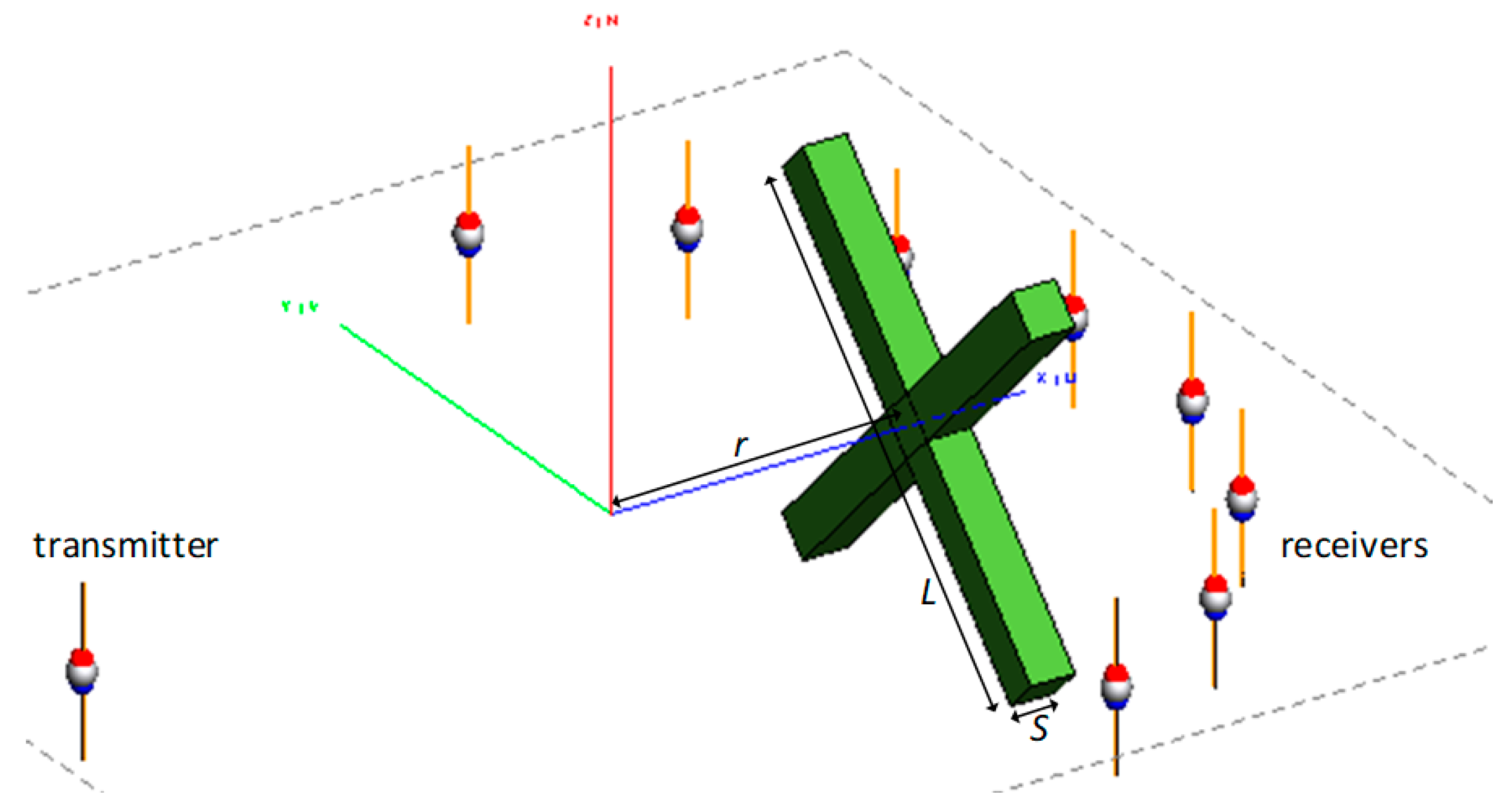
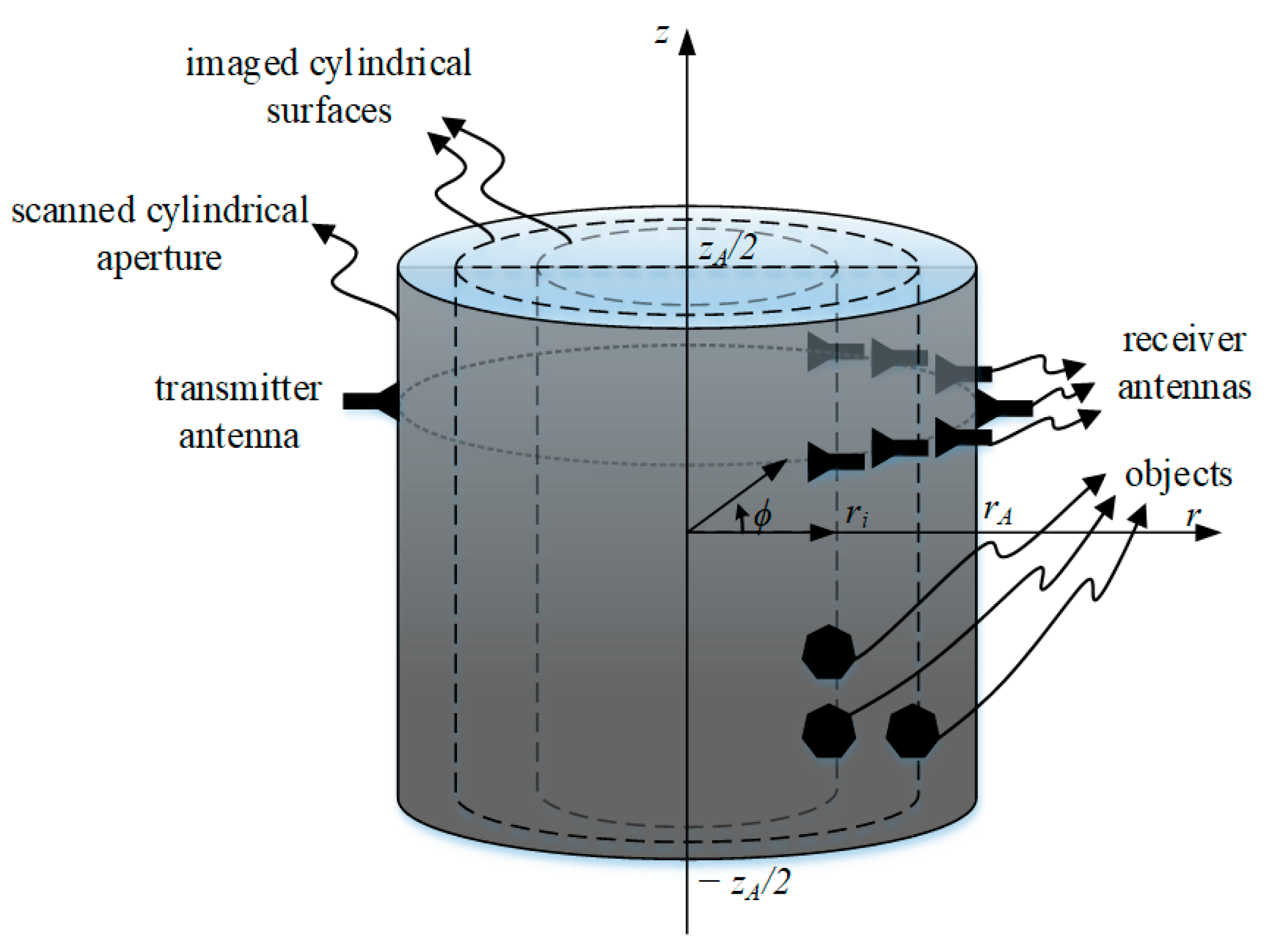
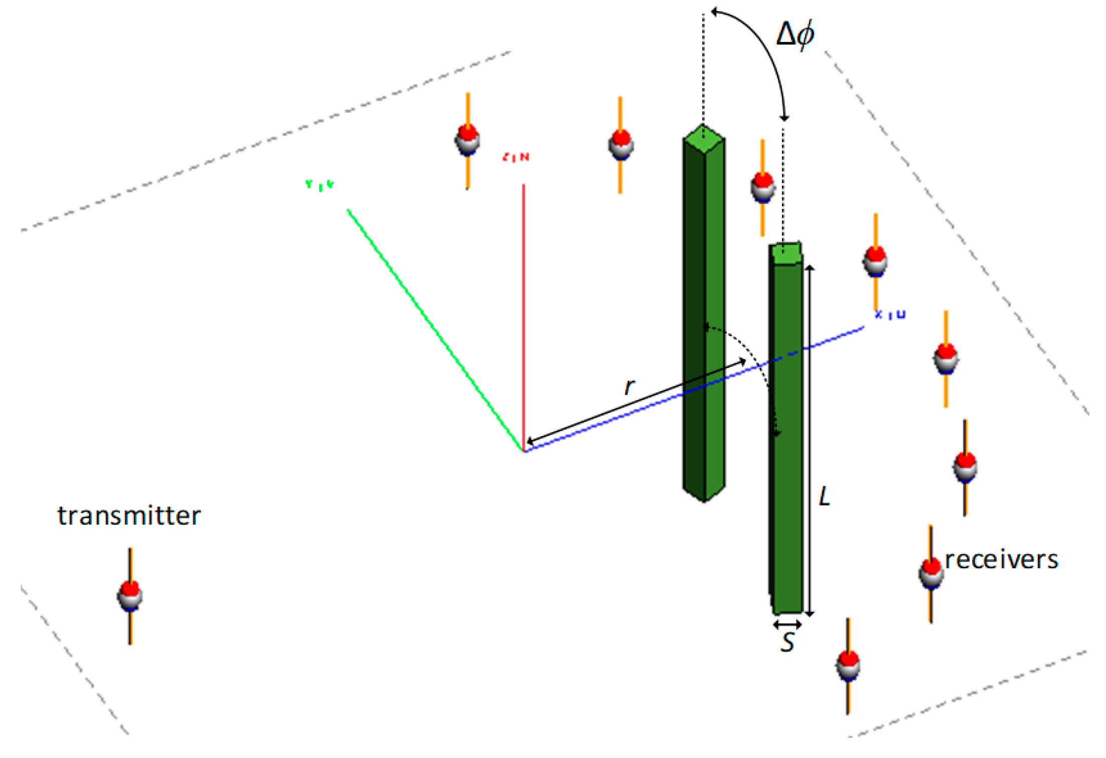
Figure 1 illustrates the proposed microwave imaging setup including a transmitter antenna to illuminate objects and an array of $N_A$ receiver antennas that scans the scattered fields. The transmitter antenna and the array of receiver antennas scan a cylindrical aperture with radius of $r_A$ and height of $z_A$. The scattered field is recorded at $N_{\varphi }$ angles along the azimuthal direction $\varphi$ (within [0, 2π]) and at $N_z$ positions along the longitudinal direction $z$. The complex-valued scattered field $E^{sc}(\varphi ,z)$ is measured, at each sampling position, at $N_{\omega }$ frequencies within the narrow band of ${\omega }_1$ to ${\omega }_{N_{\omega }}$, by each receiver. The image reconstruction process then provides images over cylindrical surfaces with radii $r_i$, where $i=1,\dots ,N_r$ and $r_i$ is within (0,$r_A$). It is worth noting that the imaging system is assumed to be linear and space-invariant (LSI). The use of Born approximation for the scattering integral leads to the linear property of the imaging system [15].

For implementation of the holographic imaging, first, the responses $E^{sc,co}$ due to small objects called calibration objects (COs) placed at ($r_i$,0,0), $i=1,\dots ,N_r$, are recorded. CO is the smallest object with the largest possible contrast with respect to the background medium that can be measured by the system. It approximates an impulse function (Dirac delta function) as an input for the imaging system. The scattered response recorded for a CO placed at ($r_i$,0,0) is denoted by $E_i^{sc,co}(\varphi ,z)$ which approximately represents the point-spread function (PSF) of the imaging system. PSF is the impulse response of the system, i.e., the response collected for a point-wise object (here, named CO) which approximates an impulse function as an input for the imaging system. Then, the response due to objects under test (OUT) $E^{sc}(\varphi ,z)$ can be written as the sum of responses due to objects at cylindrical surfaces $r=r_i,i=1,\dots ,N_r$. The object response at each cylindrical surface, in turn, can be written, according to the convolution theory, as the convolution of the collected PSF for that cylindrical surface $E_i^{sc,co}(\varphi ,z)$ with the contrast function of the object over that surface $f_i(\varphi ,z)$. This is written as:

$$E^{sc}(\varphi ,z)={\displaystyle \sum _{i=1}^{N_r}{E}_i^{sc}(\varphi ,z)}={\displaystyle \sum _{i=1}^{N_r}{E}_i^{sc,co}(\varphi ,z){\ast }_{\varphi }{\ast }_z{f}_i(\varphi ,z)}$$

(1)

In Equation (1), PSF functions $E_i^{sc,co}(\varphi ,z)$ are known due to the measurement or simulation of the CO responses. This indicates that a database of PSFs is built a priori for the relevant background medium and imaged surfaces inside them by placing a CO at on that surface and recording the responses over the aperture. Such a database can be created either through measurements or simulations. Then, the recorded PSFs will be employed in the imaging of unknown objects. Besides, $E^{sc}(\varphi ,z)$ is known due to the recording of the response for the OUT. The goal is then to estimate the contrast functions of objects $f_i(\varphi ,z)$. To provide more data for image reconstruction, measurements can be implemented at multiple frequencies (over a narrow-band), ${\omega }_n$, n = 1, …, $N_{\omega }$ and multiple receivers, $a_m$, m = 1, …, $N_A$. Thus, for each receiver $a_m$, Equation (1) can be re-written at all the frequencies to provide the following system of Equations:

$$\{\begin{array}{c}{E}_{a_m}^{sc}(\varphi ,z,{\omega }_1)={\displaystyle \sum _{i=1}^{N_r}{E}_{i,a_m}^{sc,co}(\varphi ,z,{\omega }_1){\ast }_{\varphi }{\ast }_z{f}_i(\varphi ,z)}\\ ⋮\\ E_{a_m}^{sc}(\varphi ,z,{\omega }_{N_{\omega }})={\displaystyle \sum _{i=1}^{N_r}{E}_{i,a_m}^{sc,co}(\varphi ,z,{\omega }_{N_{\omega }}){\ast }_{\varphi }{\ast }_z{f}_i(\varphi ,z)}\end{array}$$

(2)

We can get such systems of equations for each receiver $a_m$, m = 1, …, $N_A$, and then combine all these systems of equations since they share the same unknown parameters $f_i(\varphi ,z)$, $i=1,\dots ,N_r$. In order to solve the system of equations we transform the equations to the spatial frequency domain. In ref. [14], doing such transformation is straight-forward along x and y directions. However, here, the functions are periodic along $\varphi$ direction. This necessitates modification of the processing.

Let us first consider the spatially-sampled versions of $E_{a_m}^{sc}(\varphi ,z,{\omega }_n)$, $E_{i,a_m}^{sc,co}(\varphi ,z,{\omega }_n)$, and $f_i(\varphi ,z)$ denoted by $E_{a_m}^{sc}(n_{\varphi },n_z,{\omega }_n)$, $E_{i,a_m}^{sc,co}(n_{\varphi },n_z,{\omega }_n)$, and $f_i(n_{\varphi },n_z)$, $n_{\varphi }=1,\dots ,N_{\varphi }$ and $n_z=1,\dots ,N_Z$, with spatial and angular intervals denoted by $\Delta z$ and $\Delta \varphi$, respectively. Thus, the convolutions in Equation (1) can be written in spectral domain as [24]:

$${\mathrm{DTFT}}_{z,\varphi }\{E_{a_m}^{sc}(n_{\varphi },n_z,{\omega }_n)\}={\displaystyle \sum _{i=1}^{N_r}{\mathrm{DTFT}}_{z,\varphi }\{E_{i,a_m}^{sc,co}(n_{\varphi },n_z,{\omega }_n)\}{\mathrm{DTFT}}_{z,\varphi }\{f_i(n_{\varphi },n_z)\}}$$

(3)

where ${\mathrm{DTFT}}_{z,\varphi }$ denotes discrete time FT (DTFT) along azimuthal and longitudinal directions, respectively. Sequences $E_{a_m}^{sc}(n_{\varphi },n_z,{\omega }_n)$, $E_{i,a_m}^{sc,co}(n_{\varphi },n_z,{\omega }_n)$, and $f_i(n_{\varphi },n_z)$ are aperiodic along the longitudinal direction z. The number of samples along z, namely $N_z$, is taken sufficiently large such that the values outside the sampled window are negligible. Their DTFT is, however, a periodic function versus the spatial frequency variable $k_z$ (corresponding to z), with period of $1/\Delta z$. Besides, these DTFTs are periodic sums of the FT of their corresponding continuous functions. Thus, the value of the continuous FT of these functions (with negligible aliasing from the adjacent terms) can be obtained from DTFT values within the range $[-1/(2\Delta z),+1/(2\Delta z)]$, provided that $\Delta z$ is sufficiently small. The DTFTs with respect to $z$ are denoted by ${\tilde{E}}_{a_m}^{sc}(n_{\varphi },k_z,{\omega }_n)$, ${\tilde{E}}_{i,a_m}^{sc,co}(n_{\varphi },k_z,{\omega }_n)$, and ${\tilde{f}}_i(n_{\varphi },k_z)$. Since these functions are periodic along $\varphi$, the convolution along that direction can be considered as a circular convolution [24]. Then, the DTFTs for the $N_{\varphi }$-periodic sequences along $\varphi$ are computationally reduced to discrete Fourier transforms (DFT) of these sequences [24]. The DFTs with respect to the $\varphi$ variable for sequences ${\tilde{E}}_{a_m}^{sc}(n_{\varphi },k_z,{\omega }_n)$, ${\tilde{E}}_{i,a_m}^{sc,co}(n_{\varphi },k_z,{\omega }_n)$, and ${\tilde{f}}_i(n_{\varphi },k_z)$ are denoted by ${\tilde{\tilde{E}}}_{a_m}^{sc}(k_{\varphi },k_z,{\omega }_n)$, ${\tilde{\tilde{E}}}_{i,a_m}^{sc,co}(k_{\varphi },k_z,{\omega }_n)$, and ${\tilde{\tilde{f}}}_i(k_{\varphi },k_z)$, where $k_{\varphi }$ is an integer from 0 to $N_{\varphi }-1$.

Using the transformations discussed above at all the frequencies for each receiver $a_m$ leads to the following system of equations at each spatial frequency pair $\kappa =(k_{\varphi },k_z)$:

$$\{\begin{array}{c}{\tilde{\tilde{E}}}_{a_m}^{sc}(\kappa ,{\omega }_1)={\displaystyle \sum _{i=1}^{N_r}{\tilde{\tilde{E}}}_{i,a_m}^{sc,co}(\kappa ,{\omega }_1){\tilde{\tilde{f}}}_i(\kappa )}\\ ⋮\\ {\tilde{\tilde{E}}}_{a_m}^{sc}(\kappa ,{\omega }_{N_{\omega }})={\displaystyle \sum _{i=1}^{N_r}{\tilde{\tilde{E}}}_{i,a_m}^{sc,co}(\kappa ,{\omega }_{N_{\omega }}){\tilde{\tilde{f}}}_i(\kappa )}\end{array}$$

(4)

After combining the systems of equations for all the $N_A$ receivers, the following system of equations is obtained at each spatial frequency pair $\kappa =(k_{\varphi },k_z)$:

$${\widetilde{\tilde{\underset{\_}{E}}}}^{sc}=\tilde{\widetilde{\underset{\_}{\underset{\_}{D}}}}\underset{\_}{F}$$

(5)

where

$${\widetilde{\tilde{\underset{\_}{E}}}}^{sc}=\left[\begin{array}{c}{\widetilde{\tilde{\underset{\_}{E}}}}_1^{sc}\\ ⋮\\ {\widetilde{\tilde{\underset{\_}{E}}}}_{N_A}^{sc}\end{array}\right]\underset{\_}{\widetilde{\tilde{\underset{\_}{D}}}}=\left[\begin{array}{c}{\widetilde{\tilde{\underset{\_}{D}}}}_1\\ ⋮\\ {\widetilde{\tilde{\underset{\_}{D}}}}_{N_A}\end{array}\right]\widetilde{\tilde{\underset{\_}{F}}}=\left[\begin{array}{c}{\tilde{\tilde{f}}}_1(\kappa )\\ ⋮\\ {\tilde{\tilde{f}}}_{N_r}(\kappa )\end{array}\right]$$

(6)

And

$${\widetilde{\tilde{\underset{\_}{E}}}}_{a_m}^{sc}=\left[\begin{array}{c}{\tilde{\tilde{E}}}_{a_m}^{sc}(\kappa ,{\omega }_1)\\ ⋮\\ {\tilde{\tilde{E}}}_{a_m}^{sc}(\kappa ,{\omega }_{N_{\omega }})\end{array}\right],{\underset{\_}{\tilde{\tilde{D}}}}_{a_m}=\left[\begin{array}{ccc}{\tilde{\tilde{E}}}_{1,a_m}^{sc,co}(\kappa ,{\omega }_1)& \cdots & {\tilde{\tilde{E}}}_{N_r,a_m}^{sc,co}(\kappa ,{\omega }_1)\\ ⋮& \ddots & ⋮\\ {\tilde{\tilde{E}}}_{1,a_m}^{sc,co}(\kappa ,{\omega }_{N_{\omega }})& \cdots & {\tilde{\tilde{E}}}_{N_r,a_m}^{sc,co}(\kappa ,{\omega }_{N_{\omega }})\end{array}\right]$$

(7)

These systems of equations are solved at each spatial frequency pair $\kappa =(k_{\varphi },k_z)$ to obtain the values for ${\tilde{\tilde{f}}}_i(\kappa )$, $i=1,\dots ,N_r$. Then, inverse DTFT along longitudinal direction $z$ and inverse DFT along azimuthal direction $\varphi$ can be applied to reconstruct images $f_i(n_{\varphi },n_z)$ over all cylindrical surfaces $r=r_i$, $i=1,\dots ,N_r$. At the end, the normalized modulus of $f_i(n_{\varphi },n_z)$, $|f_i(n_{\varphi },n_z)|/M$, where $M$ is the maximum of $|f_i(n_{\varphi },n_z)|$ for all $r_i$, is plotted versus $\varphi$ and $z$ to obtain 2D images of the objects at all $N_r$ cylindrical surfaces. By putting together all 2D images, a 3D image of the objects is obtained. We call this process normalization of the images.

3. Simulation Results

In this section, we present the imaging results obtained from applying the proposed holographic imaging technique on the data simulated in FEKO which is a high frequency electromagnetic simulation software [25]. For 2D imaging, we conduct the simulations to collected data when the transmitter and receivers antennas rotate ${360}^{°}$ around the objects. For 3D imaging, in addition to the azimuthal rotation as mentioned above, the transmitter and receivers antennas scan together along z direction as well. Further details are mentioned in the following subsections. First, we show the performance of the technique in 2D imaging and study the effect of number of frequencies and object size. Then, we demonstrate the satisfactory performance of the technique by 3D imaging examples.

3.1. 2D Imaging with Single-Frequency Data

Figure 2 shows the FEKO simulation setup consisting of one transmitter antenna and eight receiver antennas rotating together on a circle of radius $R=60$ mm. The antennas are resonant dipoles. The azimuthal angle between the receiver antennas is $\Delta {\varphi }_a={20}^{°}$ Properties of the background medium are ${\epsilon }_r=22$ and $\sigma =1.25$ S/m. We perform imaging over three circles with radii of $r_1=24\mathrm{mm}$, $r_2=36\mathrm{mm}$, and $r_3=48\mathrm{mm}$. The objects are cubes of size D = 3 mm. There are two objects at $r_1$ with angular separation of $\Delta {\varphi }_1={40}^{°}$, one object at $r_2$, and two objects at $r_3$ with angular separation of $\Delta {\varphi }_3={60}^{°}$. The properties of objects are ${\epsilon }_r=55$ and $\sigma =4$ S/m. Data is collected at 181 samples along the azimuthal direction (every $2^{°}$) and at 1.7 GHz.

The reconstructed images over three circles with radii of 24 mm, 36 mm and 48 mm are shown in Figure 3. On the circle with radius $r_3=48\mathrm{mm}$, two high-level peaks are observed at $\pm {20}^{°}$ which means that two cubes on the outer circle can be reconstructed well. On the middle circle with radius of $r_2=36\mathrm{mm}$, one high-level peak is observed at 0 degree correctly representing an object at that position. However, many high-level artifacts are present compared to the reconstructed image on the outer circle. The reconstructed image on the inner circle with radius of $r_1=24\mathrm{mm}$ shows no distinct high-level peaks representing the objects.

3.2. 2D Imaging with Double Frequency Data

In order to improve the quality of the reconstructed images, double frequency data is collected by eight receiver antennas. With more frequency information, better reconstructed images are expected.

Figure 4 shows the reconstructed images when using double frequency data at 1.5 GHz and 1.9 GHz. Compared to the images shown in Figure 3, it is observed that when using double frequency data, the reconstructed image on the circle with radius of $r_3=48\mathrm{mm}$ has better quality showing two distinct peaks representing the presence of the two objects on that circle and lower level of artifacts. The reconstructed image on the middle circle also shows lower level of artifacts compared to those in Figure 3 and the high-level peak representing the object on that circle has better quality.

On the inner circle with a radius of $r_1=24\mathrm{mm}$, two peaks are observed at $\pm {30}^{°}$. This indicates that the two cubes on the inner circle can be reconstructed when double frequency data is collected although we still observe some high level of artifacts on this circle.

3.3. 2D Imaging of Larger Objects

In order to see the effect of size of the objects on the quality of the reconstructed images, we increase the size of objects in Figure 2 to D = 5 mm and 10 mm. The images in this section are reconstructed with data collected at 1.5 GHz and 1.9 GHz.

The reconstructed images for object sizes of $D=5\mathrm{mm}$ are shown in Figure 5. By comparing these results with those in Figure 4, we conclude that the quality of the reconstructed images is better, in particular, for the imaged circle with radius of $r_1=24\mathrm{mm}$. The levels of the artifacts on the imaged circles with radii of $r_1=24\mathrm{mm}$ and $r_2=36\mathrm{mm}$ get much lower than those in Figure 4.

Next, we increase the size of objects to $D=10\mathrm{mm}$. Figure 6 shows the reconstructed images for this case. Compared to the reconstructed images of objects with $D=5\mathrm{mm}$, the quality of the reconstructed images gets worse. On the imaged circle with radius of $r_2=36\mathrm{mm}$, two peaks are observed which might be the shadow of objects on the imaged circle with radius of $r_3=48\mathrm{mm}$. On the imaged circle with radius of $r_1=24\mathrm{mm}$, the objects at $\pm {30}^{°}$ are not reconstructed well and the image includes many spurious peaks. The degradation of the imaging quality is mainly due to the use of Born approximation in holographic imaging which indicates that the image reconstruction quality deteriorates for larger or higher contrast objects [15].

3.4. Study of the Imaging Quality

In this section, we study the quality of the imaging process when using single frequency data, double frequency data, and when a single object with sizes of 3 mm, 5 mm, and 10 mm is placed on circles with radii of $r_1=24\mathrm{mm}$, $r_2=36\mathrm{mm}$, and $r_3=48\mathrm{mm}$. To evaluate the quality of the reconstructed images, we define a reconstruction error $E_T$ parameter as:

$$E_T={\displaystyle \sum _{i=1}^{N_r}\Vert |f_i(n_{\varphi },n_z)|/M-f_{i,ideal}(n_{\varphi },n_z)\Vert }$$

(8)

where $f_{i,ideal}(n_{\varphi },n_z)$ is the ideal image for which the values are all 0 except being 1 at the true positions of the objects.

Form

Table 1. Reconstruction error when using single frequency data.

Size	r = 48 mm	r = 36 mm	r = 24 mm
D = 3 mm	7.62	9.12	10.73
D = 5 mm	9.52	9.64	11.83
D = 10 mm	10.55	13.15	13.52

and

Table 2. Reconstruction error when using double frequency data.

Size	r = 48 mm	r = 36 mm	r = 24 mm
D = 3 mm	6.41	6.91	8.86
D = 5 mm	6.44	8.52	8.90
D = 10 mm	8.08	8.85	9.23

, it is observed that the quality of the imaging degrades for inner circles. This has been notified in the previous works as well (e.g., see ref. [18]). Also, it is observed that the quality of the imaging improves when using double frequency data compared to single frequency data.

3.5. 3D Imaging with Double Frequency Data and Eight Receivers

Figure 7 shows the FEKO simulation model for the first 3D imaging example. The transmitter-receivers configuration, number of antennas, properties of the background and objects are similar to those in Figure 2. The objects are two cuboids with square cross-section of size S = 4 mm and height of L = 67.5 mm. The angular separation between the cuboids is $\Delta \varphi ={40}^{°}$ and they are placed at radius of $r=36\mathrm{mm}$. In order to have a realistic study, we add White Gaussian noise with signal-to-noise ratio (SNR) of 30 dB to the simulated data. Scanning step along the azimuthal direction is the same as in the 2D imaging simulations. Along $z$ axis scanning is performed at 21 steps over $-5\lambda$ to $5\lambda$, where $\lambda$ is the wavelength at center frequency 1.7 GHz. Data is collected at 1.5 GHz and 1.9 GHz. Image reconstruction is implemented over three cylindrical surfaces at $r_1=24\mathrm{mm}$, $r_2=36\mathrm{mm}$, and $r_3=48\mathrm{mm}$. Sample raw responses for the 4th receiver (in the middle), at frequency of 1.5 GHz, and for PSFs for $r_1=24\mathrm{mm}$, $r_2=36\mathrm{mm}$, and $r_3=48\mathrm{mm}$ for object response are shown in Figure 8. Figure 9 shows the reconstructed images. Two cuboids on the middle surface are reconstructed well. Two bright lines are observed at $\pm 20$° on the middle surface and the extent of them along the $z$ axis is consistent with the actual height of the objects. This clearly shows the capability of the proposed imaging technique in reconstruction of 3D images using narrow-band microwave data.

Figure 10 shows the FEKO simulation model for the second 3D imaging example. The transmitter-receivers configuration, number of antennas, properties of the background medium and objects are similar to those in Figure 2. There is an X-shaped object with square cross-section of size S = 4 mm and length of arms L = 56.25 mm. It is placed at radius of $r=36\mathrm{mm}$ with its arms rotated ${45}^{°}$ with respect to the $x$ and $z$ axes. Similar to the previous example, in order to have a realistic study, we add White Gaussian noise with signal-to-noise ratio (SNR) of 30 dB to the simulated data. Scanning step along the azimuthal direction is the same as in the 2D imaging simulations. Along $z$ axis scanning is performed at 21 steps over $-5\lambda$ to $5\lambda$, where $\lambda$ is the wavelength at center frequency 1.7 GHz. Data is collected at 1.5 GHz and 1.9 GHz. Image reconstruction is implemented over three cylindrical surfaces at $r_1=24\mathrm{mm}$, $r_2=36\mathrm{mm}$, and $r_3=48\mathrm{mm}$. Figure 11 shows the reconstructed images. The X-shaped object is reconstructed well at the middle-imaged surface confirming the satisfactory performance of the proposed imaging technique.

3.6. Resolution along Azimuthal and Longitudinal Directions

Figure 12 shows the normalized 1D slices along ϕ and z directions for the 3D reconstructed images of a single object placed at $r_3=48\mathrm{mm}$, $r_2=36\mathrm{mm}$, and $r_1=24\mathrm{mm}$ (obtained from three separate image reconstruction processes). The resolution is evaluated by computing the distance bounded by two points on the image on opposite sides of the peak and marked by 0.7 times the peak value. This corresponds to approximately 6 mm and 14 mm along the azimuthal and longitudinal directions, respectively, and it is approximately similar for all the radii (only slight degradation in the order of 1 mm or 2 mm is observed for the smaller radii compared to larger ones). The resolution along azimuthal direction has been evaluated by Δϕ in radian multiplied by the radius for the corresponding surface, where Δϕ is the angular width of the 0.7 level discussed above. That is why although the angular widths of the 0.7 levels look different in Figure 12a–c, they all lead to approximately similar azimuthal resolutions. Please note that to have a realistic evaluation of the resolution, the data has been corrupted with noise of SNR = 30 dB.

3.7. Study the Effect of Noise

In order to study the effect of noise on the reconstructed images, in this section we present the results for the 3D imaging example in Figure 10 with the results shown with noise of SNR = 30 dB in Figure 11. Here, we decrease SNR to 20 dB and 10 dB. Figure 13 shows the reconstructed images. It is observed that with SNR = 20 dB, the results are still satisfactory but with SNR = 10 dB the quality of the images deteriorates significantly.

4. Experimental Results

In this section, we present the construction of a low-cost microwave data acquisition system including a transmitter unit, an in-phase quadrature (I/Q) receiver unit, a cylindrical scanning system, antennas, and computer for controlling and processing. Then, we present the 3D imaging results demonstrating the satisfactory performance of the system.

4.1. Microwave Measurement System

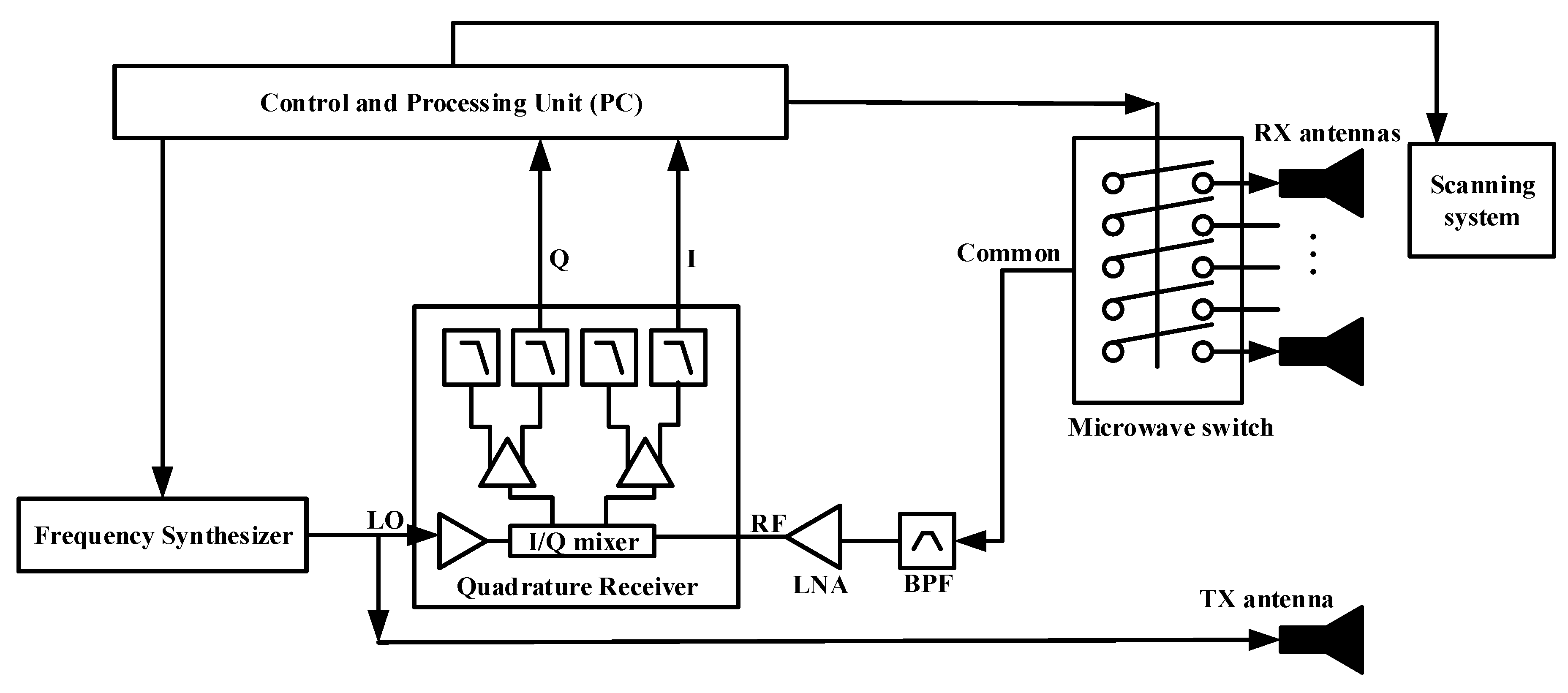
Figure 14 shows the block diagram of the constructed low-cost and compact 3D microwave holographic imaging system. For our measurements, we use a Plexiglas container including a mixture of water (20%) and glycerin (80%). According to ref. [26], this mixture has properties of approximately ${\epsilon }_r=22$ and $\sigma =1.25$ S/m within the frequency range of 1.5 GHz to 1.8 GHz which is the targeted operation range in our experimental study. We confirmed this by dielectric property measurements using a Keysight Dielectric probe kit (performance probe N1501A) together with the relevant measurement Software N1500A and a VNA (E5063A from Keysight). The liquid mixture container has diameter of 120 mm and height of 200 mm. The objects to be imaged are plastic cylinders with diameter of 18 mm and height of 50 mm covered by thin copper sheets. These objects are held inside the liquid at the desired positions with thin wooden sticks that are clipped to a cylindrical foam placed at the top of the liquid container. Imaging will be performed over cylindrical surfaces (3D imaging) at radii of $r_1=20\mathrm{mm}$, $r_2=35\mathrm{mm}$, and $r_3=50\mathrm{mm}$. 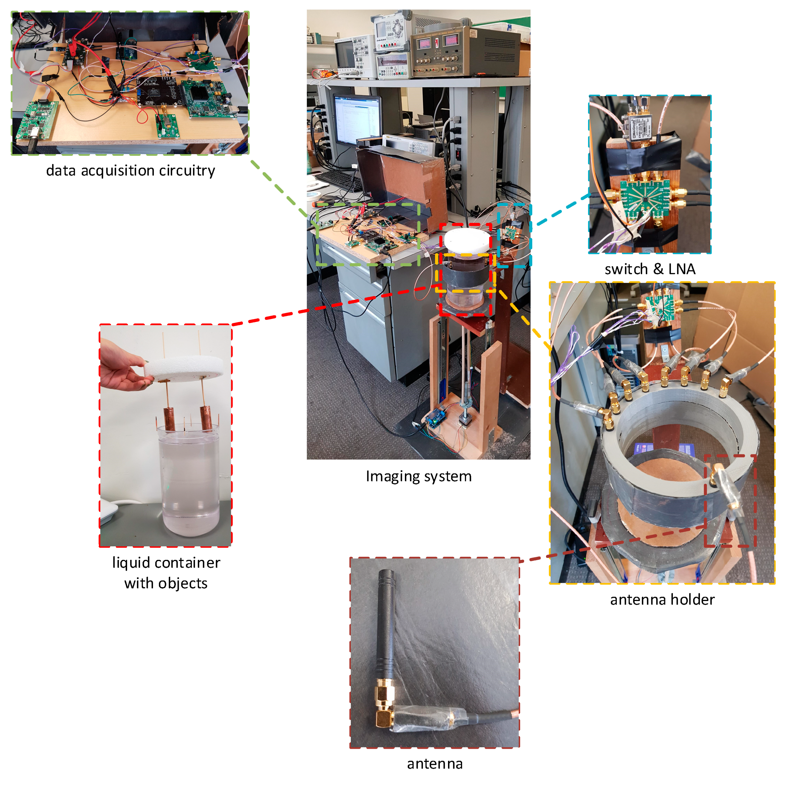Figure 15 shows the imaging system along with the zoomed view for the main components that will be described in the following. To reduce electromagnetic interferences (EMI), the data acquisition circuitry and the scanning setup are placed inside boxes covered by microwave absorbing sheets.

In the data acquisition system, a transmitter module, DC1705C from Analog Devices, with frequency range from 700 MHz to 6.39 GHz is connected to a 10 MHz precision pocket reference oscillator, PPRO30–10.000 from Crystek Corporation, which provides a reference frequency. A USB serial controller, DC590B from Analog Devices, is connected to DC1705C so that the transmitter unit can be controlled by PC via MATLAB software [27]. The output of the transmitter unit is connected to a variable gain amplifier (VGA), ADL5330 from Analog Devices, operating from 10 MHz to 3 GHz which is then connected to a transmitter antenna. In this way, a microwave signal can be transmitted with variable frequencies and powers to illuminate the imaged medium.

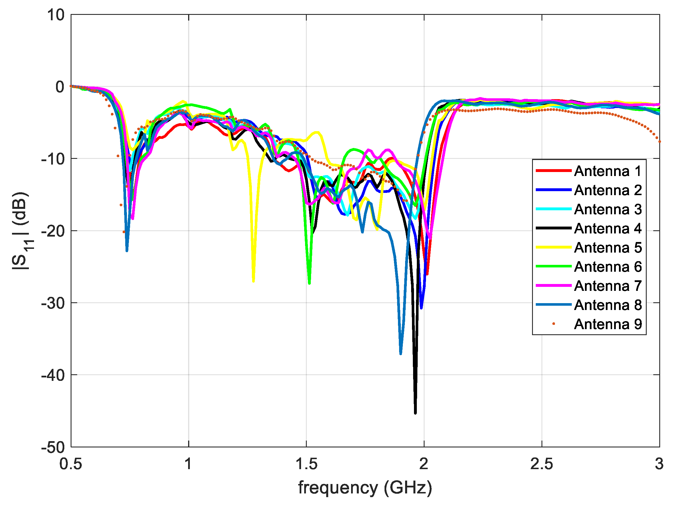
For transmitting and receiving the microwave power, we employ commercial monopole antennas, Mini GSM/Cellular Quad-Band Antenna-2 dBi SMA Plug from Adafruit Co., covering frequency bands of 850/900/1800/1900/2100 MHz. Figure 16 shows the measured $\left|S_{11}\right|$ (by VNA) for the nine antennas used as transmitter and receivers. These measurements are performed while the antennas are placed in a 3D-printed holder around the liquid container. The values of $\left|S_{11}\right|$ are mostly below $-10 \mathrm{dB}$ over the targeted operation band of 1.5 GHz to 1.8 GHz.

The receiver unit of the data acquisition system includes a 14-Bit, 125 Msps Direct Conversion Receiver, DC1513B-AB from Analog Devices, which has a frequency range from 0.7 to 2.7 GHz. To control this receiver unit with PC, this unit is connected to a USB data acquisition controller, DC890B from Analog Devices. The clock source for the receiver board DC1513B-AB is provided by High Speed ADC Clock Source, DC1216A-C from Analog Devices, with clock speed of 80 MHz.

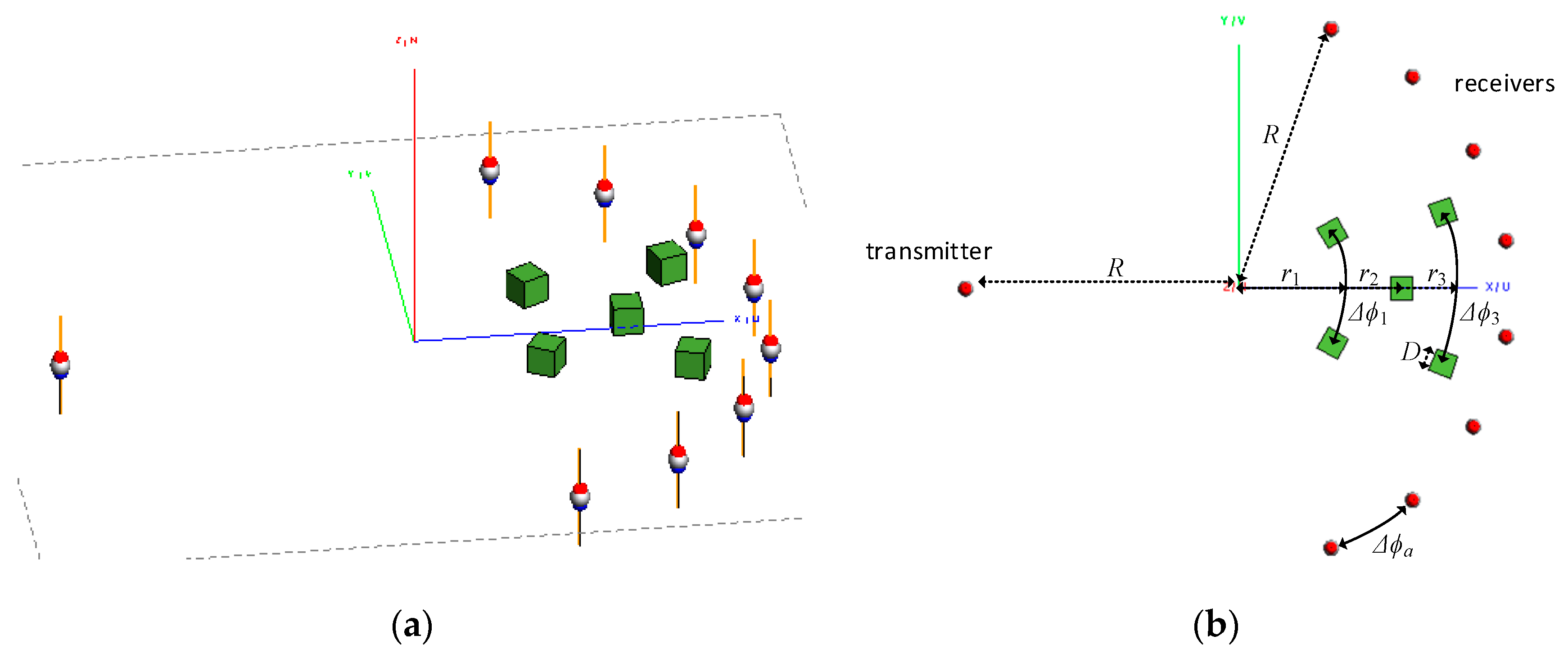
One output of the transmitter is connected to a 6 dB attenuator, CATTEN-06R0 form Crystek Corporation, covering 0 GHz to 3 GHz, and used as referenced signal for the receiver unit. Eight receiver antennas are connected to an RF SP8T switch, EV1HMC321ALP4E from Analog Devices, that operates from 0 to 8 GHz. This switch is controlled by an Arduino Uno demo board controlled by MATLAB. Received signal after the switch is fed to the receiver unit through a wideband low-noise amplifier (LNA), ZX60-33LN-S+ from Mini-Circuits, operating from 50 MHz to 3 GHz, as well as a bandpass filter (BPF), VBFZ-1690-S+ from Mini-Circuits, covering 1455 MHz to 1925 MHz The transmitter and receiver units are powered separately via high-precision lab power supplies. All ground pins are connected to a common ground pin. The transmitter antenna and the receiver antenna arrays are placed on opposite sides of the container similar to the simulation setup in Figure 2. The angular separation between the receiver antennas is also similar to the simulation study, i.e., $\Delta {\varphi }_a={20}^{°}$.

The cylindrical scanning system contains two stepper motors, NEMA 17 from Adafruit, connected, via an Arduino stepper motor shield board and an Arduino Uno board, to computer to be controlled via MATLAB. One of the motors moves the container along the longitudinal direction and the other one moves that along the azimuthal direction from $0^{°}$ to ${360}^{°}$. The antennas are stationary and placed on an antenna holder which has been custom-designed and 3D-printed in our lab.

To control the whole system using computer, a MATLAB code has been developed that performs the following tasks: (1) control the transmitter, (2) control the switch, (3) control the receiver unit and acquire data, (4) control motors, and (5) implement holographic imaging. In the following we briefly describe each part.

Transmitter code controls the transmitter unit and generates the signal at two frequencies, 1.5 GHz and 1.8 GHz. To set two frequencies, the Serial Port Register Contents in the DC1705C board are written through serial peripheral interface (SPI) bus.

Switch code is used to select which of the eight receiver antennas is connected to the receiver unit to collect data. Three of the output pins on the Arduino Uno demo board are connected to three control pins on the switch. By setting the voltage level for each pin according to the truth table of the switch, one of the antennas can be chosen at a time to collect data.

The main body of the receiver unit code is used to collect data from two channels of the I/Q receiver unit, one channel providing the real part and another the imaginary part. These two parts are combined in MATLAB to form a complex number. Thus, at each sampling position, we collect two complex numbers corresponding to two frequencies of 1.5 GHz and 1.8 GHz for each antenna. Also, to make the measurements more robust to noise, we collect 4096 samples for each channel (real and imaginary channels), per position, per frequency, and per antenna. Since the local oscillator (LO) and the radio frequency (RF) inputs of the receiver unit have the same frequency, the I/Q output signals, i.e., the intermediate frequency (IF) outputs of the receiver unit are DC signals.

Motor code controls the motors to move along the longitudinal axis and the azimuth axis from $0^{°}$ to ${360}^{°}$ in a desired speed and direction. The number of sampling positions can be changed.

The imaging code is used to implement holographic imaging. Imaging is performed over cylindrical surfaces (3D imaging) at radii of $r_1=20\mathrm{mm}$, $r_2=35\mathrm{mm}$, and $r_3=50\mathrm{mm}$.

4.2. Experimental 3D Imaging Results

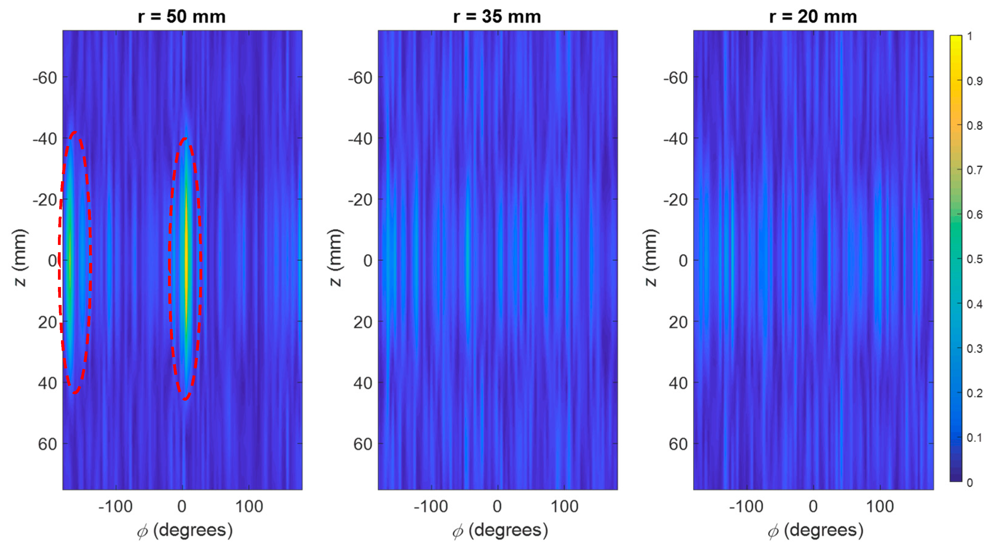
The container including the objects is scanned by the transmitter and receiver antennas over a cylindrical aperture. At each longitudinal position $z$, scanning is performed along the azimuthal direction $\varphi$ in 100 steps to cover ${360}^{°}$. Scanning along the longitudinal direction is performed over one half of a cylindrical aperture with length of 80 mm and in 10 steps. Then, due to approximate symmetry of the structure along the longitudinal direction, the other half is acquired by flipping and combining that with the first half. The complex-valued data collected by the eight receiver antennas are then processed using the 3D holographic imaging technique. In the first experiment, we place two objects on the outer surface $r_3=50\mathrm{mm}$ with, approximately, one object at $\varphi =0^{°}$ and another one at $\varphi ={180}^{°}$. 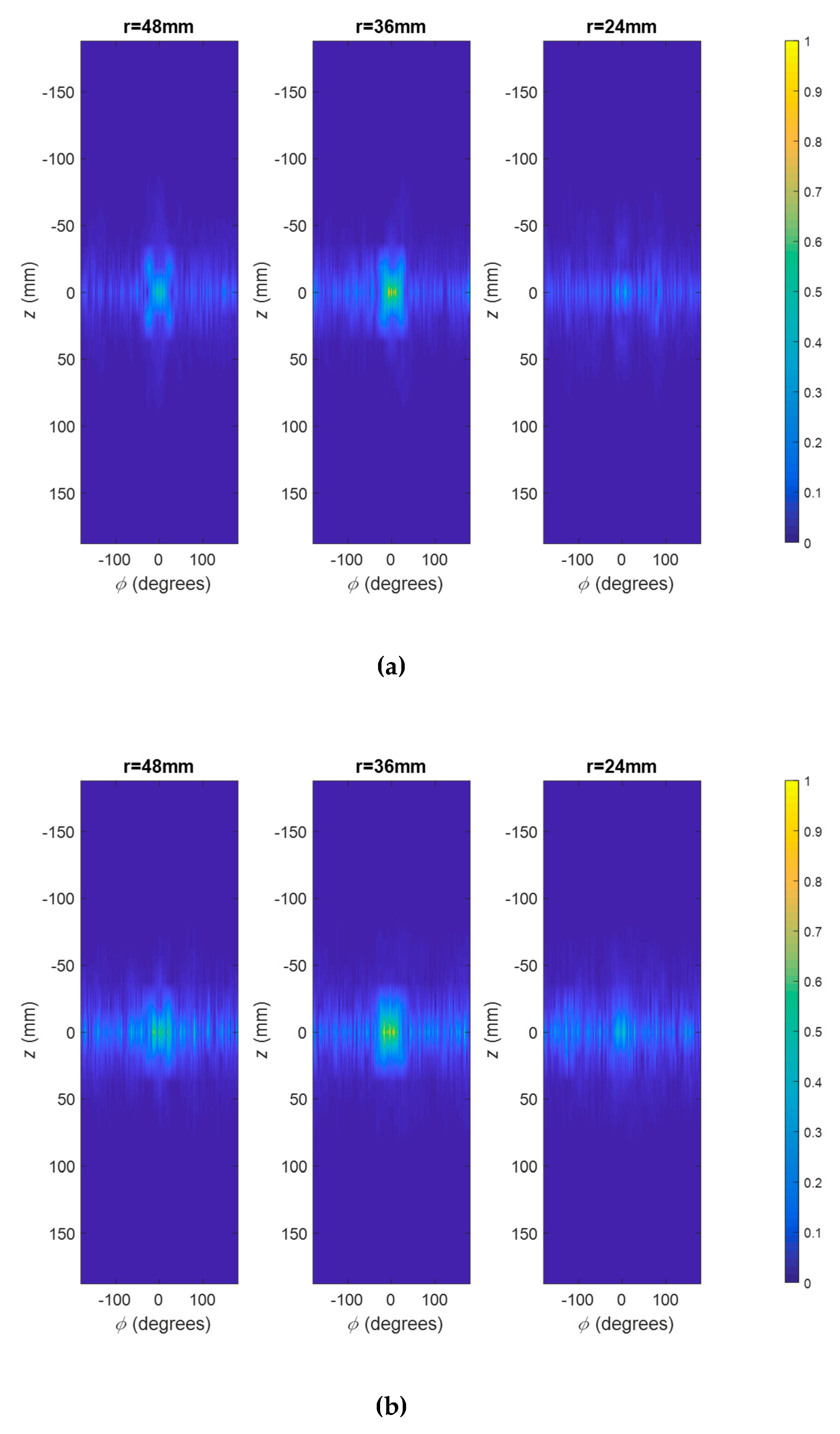Figure 17 shows the reconstructed images. It is observed that the two objects can be reconstructed well at $r_3=50\mathrm{mm}$ with the images at the other surfaces showing small artifacts. We use the reconstruction error parameter defined in Equation (8) to evaluate the quality of image reconstruction. The computed reconstruction error for this experiment is 17.92.

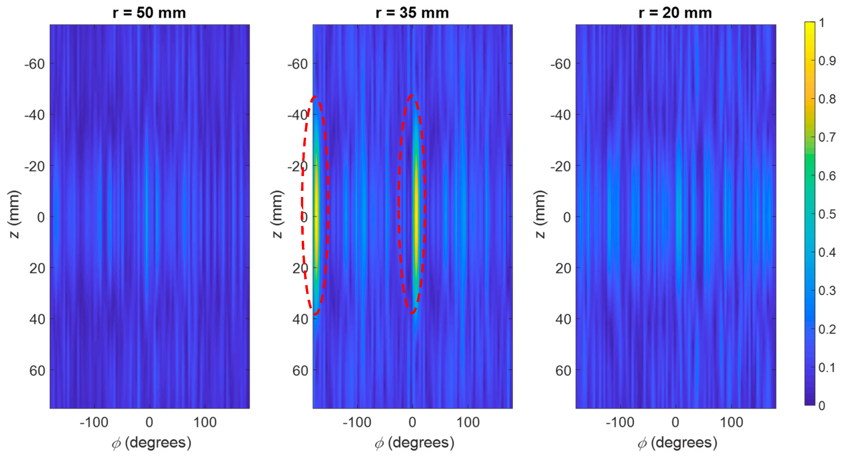
We then repeat this experiment but, this time, putting the two objects on the middle surface $r_2=35\mathrm{mm}.$ Figure 18 shows the reconstructed images over the three cylindrical surfaces for this case. Again, it is observed that the two objects on the middle surface can be reconstructed well at their true positions of $\varphi =0^{°}$ and $\varphi ={180}^{°}$. We use the reconstruction error parameter defined in Equation (8) to evaluate the quality of image reconstruction. The computed reconstruction error for this experiment is 20.84. Comparing the reconstruction error parameter with the previous example, we observe the degradation of the image quality. This is mainly due to the fact that the background medium is lossy, and the responses of the objects are weaker for the objects on the surface $r_2=35\mathrm{mm}$ compared to those at $r_3=50\mathrm{mm}$.

5. Conclusions

In this paper, we proposed a microwave imaging system capable of reconstructing 3D images of objects in the near field of the antennas. The applications are in non-destructive testing of non-metallic composite materials and biomedical imaging. To achieve low-cost, compactness, and reduce the component count for a data acquisition system, narrow-band data is acquired as opposed to the previously proposed 3D cylindrical holographic imaging techniques. An I/Q detection data acquisition system is built based on the cost-effective off-the-shelf components to replace the expensive and bulky VNAs. The system is tailored for imaging over a narrow band and this makes it much less expensive, affordable, and compact.

In this work, we used a mixture of water and glycerin which is very lossy. We selected this mixture considering both biomedical applications and non-destructive testing of the pipes which may carry mixtures of water and other substances. For microwave imaging of such media, the optimal frequency band to provide sufficient penetration while having acceptable resolution is within the range of 1 GHz to 10 GHz (e.g., see ref. [3,22,23]). This justifies the chosen frequencies in this work.

The reconstructed images using this data acquisition system confirms the satisfactory performance of this narrow-band system in 3D imaging. To evaluate the quality of the image reconstruction process, we defined a reconstruction error to compare the images with an ideal image (true image). We observed that, in general, the reconstruction error increases for reconstructing objects on surfaces farther away from the antennas. Besides, the reconstruction error decreases when using double frequency data compared to single frequency data. Furthermore, we observed that increasing the object size improves the quality of the images but there is a limit for that due to the use of Born approximation in the holographic imaging.

Although scanning of the objects over a cylindrical aperture takes a few hours, the holographic imaging technique itself is fast. Here, we provide an estimate of the computational complexity of our 3D image reconstruction process. The number of samples along ϕ and z are $N_{\varphi }$ and $N_z$, respectively. The number of receiver antennas and measurement frequencies are $N_A$ and $N_{\omega }$, respectively. The number of imaged surfaces is $N_r$. We denote the number of samples of k_z by $N_{k_z}$. The number of samples along $k_{\varphi }$ is $N_{\varphi }$.

Table 3. Details of computational complexity of the proposed image reconstruction process.

Operation	Number of Flops
FT of the scattered fields	$N_{\omega }{N}_A{N}_{\varphi }^2{N}_z\log (N_z)$
FT of PSF functions	$N_r{N}_{\omega }{N}_A{N}_{\varphi }^2{N}_z\log (N_z)$
Solving the systems of equations for all combinations of $k_{\varphi }$ and $k_z$	$N_{\varphi }{N}_{k_z}(2N_A{N}_{\omega }{N}_r^2-(2/3)N_r^3)$
Inverse FT of the contrast function	$N_r{N}_{\varphi }^2{N}_{k_z}\log (N_{k_z})$

summarizes the computational complexity of our approach. The computational complexity of solving the systems of equations has been provided with the assumption that they are solved with QR factorization. The total number of flops for the image reconstruction process is the sum of all the flops in Table 3. The 3D image reconstruction process takes 10 s on a regular PC with Intel Core i5 CPU at 3.2 GHz and 8 GB RAM.

To expedite the imaging process and move toward real-time or quasi real-time imaging, an array of antennas can be employed similar to the setups used for security screening in the airports [4].

As a final note, in this work, the goal was to propose an imaging system which is: (a) more cost-effective, (b) accessible and affordable outside microwave laboratories in various industrial or biomedical applications, and (c) compact and portable due to the fact it is tailored for measurement over a very narrow band and for a specific purpose. VNAs normally are general-purpose equipment that are capable of performing measurements over a very wideband. This makes them expensive and bulky which is not suitable for widespread use in various industrial settings. We should emphasize that the proposed system has been built with a cost of less than $1000 USD and can be made very compact by arranging the boards in a small box. The drawback of the proposed system compared to a regular VNA is lower dynamic range. For a regular modern VNA, the dynamic range at frequencies around 1 GHz to 2 GHz is around 100 dB while the dynamic range for the receiver used in our proposed system is 63.5 dB. This limits the sensitivity of the proposed system indicating that the imaged objects need to be larger to provide measurable signatures in the proposed system compared to a VNA-based measurement system.

References

1. Zoughi, R. Microwave Non-Destructive Testing and Evaluation; Kluwer: Dordrecht, The Netherlands, 2000. [Google Scholar]
2. Amin, M.G. Through-the-Wall Radar Imaging; CRC Press: Boca Raton, FL, USA, 2016. [Google Scholar]
3. Nikolova, N.K. Microwave imaging for breast cancer. IEEE Microw. Mag. 2011, 12, 78–94. [Google Scholar] [CrossRef]
4. Sheen, D.M.; McMakin, D.L.; Hall, T.E. Three-dimensional millimeter-wave imaging for concealed weapon detection. IEEE Trans. Microw. Theory Tech. 2001, 49, 1581–1592. [Google Scholar] [CrossRef]
5. Sheen, D.M.; McMakin, D.; Hall, T.E. Near-field three-dimensional radar imaging techniques and applications. Appl. Opt. 2010, 49, E83–E93. [Google Scholar] [CrossRef] [PubMed]
6. Hagemaier, D.J. Fundamentals of Eddy Current Testing; Amer Society for Nondestructive: Columbus, OH, USA, 1990. [Google Scholar]
7. Amineh, R.K.; Koziel, S.; Nikolova, N.K.; Bandler, J.W.; Reilly, J.P. A space mapping methodology for defect characterization from magnetic flux leakage measurement. IEEE Trans. Mag. 2018, 44, 2058–2065. [Google Scholar] [CrossRef]
8. Betz, C.E. Principles of Magnetic Particle Testing, 1st ed.; Magnaflux Corporation: Chicago, IL, USA, 1967. [Google Scholar]
9. Meaney, P.M.; Goodwin, D.; Golnabi, A.H.; Zhou, T.; Pallone, M.; Geimer, S.D.; Burke, G.; Paulsen, K.D. Clinical microwave tomographic imaging of the calcaneus: A first-in-human case study of two subjects. IEEE Trans. Biomed. Eng. 2012, 59, 3304–3313. [Google Scholar] [CrossRef] [PubMed]
10. Fear, E.C.; Hagness, S.C.; Meaney, P.M.; Okoniewski, M.; Stuchly, M.A. Enhancing breast tumor detection with near-field imaging. IEEE Microw. Mag. 2002, 3, 48–56. [Google Scholar] [CrossRef]
11. Xie, Y.; Guo, B.; Xu, L.; Li, J.; Stoica, P. Multistatic adaptive microwave imaging for early breast cancer detection. IEEE Trans. Biomed. Eng. 2016, 53, 1647–1657. [Google Scholar] [CrossRef] [PubMed]
12. Tobon, J.A.V.; Attardo, E.A.; Dassano, G.; Vipiana, F.; Casu, M.R.; Vacca, M.; Vecchi, G. Design and modeling of a microwave imaging system for breast cancer detection. In Proceedings of the 2015 9th European Conference on Antennas and Propagation, Lisbon, Portugal, 13–17 April 2015. [Google Scholar]
13. Semenov, S.Y.; Corfield, D.R. Microwave tomography for brain imaging: Feasibility assessment for stroke detection. Int. J. Antennas Propag. 2008, 2008, 254830. [Google Scholar] [CrossRef]
14. Amineh, R.K.; McCombe, J.; Khalatpour, A.; Nikolova, N.K. Microwave holography using point-spread functions measured with calibration objects. IEEE Trans. Instrum. Meas. 2015, 64, 403–417. [Google Scholar] [CrossRef]
15. Amineh, R.K.; Ravan, M.; Khalatpour, A.; Nikolova, N.K. Three-dimensional near-field microwave holography using reflected and transmitted signals. IEEE Trans. Antennas Propag. 2011, 59, 4777–4789. [Google Scholar] [CrossRef]
16. Amineh, R.K.; Ravan, M.; McCombe, J.; Nikolova, N.K. Three-dimensional microwave holographic imaging employing forward- scattered waves only. Int. J. Antennas Propag. 2013, 2013, 897287. [Google Scholar] [CrossRef]
17. Wu, H.; Amineh, R.K.; Ravan, M. Near-field holographic microwave imaging using data collected over cylindrical apertures. In Proceedings of the 18th Int. Symp. on Antenna Technology and Applied Electromagnetics (ANTEM), Waterloo, ON, Canada, 19−22 August 2018. [Google Scholar]
18. Amineh, R.K.; Ravan, M.; Wu, H.; Kasturi, A. Three-dimensional holographic imaging using data collected over cylindrical apertures. Microwave Opt. Technol. Lett. 2019, 61, 907–911. [Google Scholar] [CrossRef]
19. Amineh, R.K.; Nikolova, N.K.; Ravan, M. Real-Time Three-Dimensional Imaging of Dielectric Bodies Using Microwave/Millimeter Wave Holography; Wiley-IEEE Press: Hoboken, NJ, USA, 2019. [Google Scholar]
20. Bolomey, J.C.; Gardiol, F.E. Engineering Applications of the Modulated Scattering Technique; Artech House Publishers: Norwood, MA, USA, 2001. [Google Scholar]
21. Amineh, R.K.; Ravan, M.; Sharma, R.; Baua, S. Three-dimensional holographic imaging using single frequency microwave data. Int. J. Antennas Propag. 2018, 2018, 6542518. [Google Scholar] [CrossRef]
22. Marimuthu, J.; Bialkowski, K.S.; Abbosh, A.M. Software-defined radar for medical imaging. IEEE Trans. Microw. Theory Tech. 2016, 64, 643–652. [Google Scholar] [CrossRef]
23. Pagliari, D.J.; Pulimeno, A.; Vacca, M.; Tobon, J.A.; Vipiana, F.; Casu, M.R.; Solimene, R.; Carloni, L.P. A Low-cost, fast, and accurate microwave imaging system for breast cancer detection. In Proceedings of the IEEE Biomedical Circuits and Systems Conference (BioCAS), Atlanta, GA, USA, 22–24 October 2015. [Google Scholar]
24. Oppenheim, A.V.; Schafer, R.W.; Buck, J.R. Discrete-Time Signal Processing, 2nd ed.; Prentice Hall: Upper Saddle River, NJ, USA, 1999. [Google Scholar]
25. Altair-FEKO Software. Available online: https://altairhyperworks.com/product/FEKO (accessed on 14 September 2019).
26. Meaney, P.M.; Fox, C.J.; Geimer, S.D.; Paulsen, K.D. Electrical characterization of glycerin: water mixtures: Implications for use as a coupling medium in microwave tomography. IEEE Trans. Microw. Theory Tech. 2017, 65, 1471–1478. [Google Scholar] [CrossRef] [PubMed]
27. MATLAB Software, MathWorks. Available online: https://www.mathworks.com (accessed on 14 September 2019).
Figure 1. The proposed microwave imaging setup in which a transmitter antenna scans a cylindrical aperture together with an array of receiver antennas. The images are then reconstructed over cylindrical surfaces with radii r = r i .
Electronics 08 01036 g001
Figure 2. (a) Angled view of the FEKO simulation setup, and (b) Top-view of the setup consisting of one transmitter antenna and eight receiver antennas rotating together on a circle of radius R = 60 mm. The properties of the background medium are ε r = 22 and σ = 1.25   S / m . The properties of the objects are ε r = 55 and σ = 4   S / m .
Electronics 08 01036 g002
Figure 3. Normalized 2D reconstructed image of the objects with side of D = 3 mm on three imaging circles with radii of 48, 36, and 24 mm using single frequency data collected by eight receiver antennas.
Electronics 08 01036 g003
Figure 4. Normalized 2D reconstructed image of objects with side of D = 3 mm on three imaging circles with radii of 48, 36 and 24 mm using double frequency data collected by eight receiver antennas.
Electronics 08 01036 g004
Figure 5. Normalized 2D reconstructed image of objects with a side of D = 5 mm on three imaged circles with radii of 48, 36 and 24 mm using double frequency data collected by eight receiver antennas.
Electronics 08 01036 g005
Figure 6. Normalized 2D reconstructed image of objects with a side of D = 10 mm on three imaged circles with radii of 48, 36 and 24 mm using double frequency data collected by eight receiver antennas.
Electronics 08 01036 g006
Figure 7. FEKO simulation model for the first 3D imaging example. The transmitter-receivers configuration, number of antennas, properties of the background and objects are similar to those in Figure 2. The objects are two cuboids with square cross-section of size S = 4   mm and height of L = 67.5 mm. The angular separation between the cuboids is Δ ϕ = 40 ° and they are placed at radius of r = 36 mm.
Electronics 08 01036 g007
Figure 8. Sample raw responses for the 4th receiver (in the middle) and at frequency of 1.5 GHz: (a) point-spread function (PSF) for r = 48 mm, (b) PSF for r = 36 mm, (c) PSF for r = 24 mm, and (d) objects response.
Electronics 08 01036 g008
Figure 9. Normalized 3D reconstructed image of the objects shown in Figure 7 on three imaged surfaces at radii of 48, 36, and 24 mm using double frequency data collected by eight receiver antennas.
Electronics 08 01036 g009
Figure 10. FEKO simulation model for the second 3D imaging example. The transmitter-receivers configuration, number of antennas, properties of the background and objects are similar to those in Figure 2. There is an X-shape object with square cross-section of size S = 4   mm and length of each arm of L = 56.25   mm . It is placed at radius of r = 36   mm with its arms rotated 45 ° with respect to the x and z axes.
Electronics 08 01036 g010
Figure 11. Normalized 3D reconstructed image of the object in Figure 10 on three imaged surfaces at radii of 48, 36, and 24 mm using double frequency data collected by eight receiver antennas.
Electronics 08 01036 g011
Figure 12. Depiction of 1D slices of 3D reconstructed images of a single object placed: (a) at 48 mm, slice along ϕ direction, (b) at 36 mm, slice along ϕ direction, (c) at 24 mm, slice along ϕ direction, (d) at 48 mm, slice along z direction, (e) at 36 mm, slice along z direction, (f) at 24 mm, slice along z direction.
Electronics 08 01036 g012aElectronics 08 01036 g012b
Figure 13. Reconstructed 3D images of the object shown in Figure 11 when the data is corrupted by noise of: (a) SNR = 20 dB and (b) SNR = 10 dB.
Electronics 08 01036 g013
Figure 14. Block diagram of the imaging system.
Electronics 08 01036 g014
Figure 15. Imaging system with its main components.
Electronics 08 01036 g015
Figure 16. Measured | S 11 | for the nine antennas used as transmitter and receivers.
Electronics 08 01036 g016
Figure 17. Normalized 3D reconstructed image of the objects on the outer surface for three imaged surfaces at radii of 50, 35, and 20 mm using double frequency data collected by eight receiver antennas. The red dashed lines show the reconstructed objects.
Electronics 08 01036 g017
Figure 18. Normalized 3D reconstructed image of the objects on the middle surface for three imaged surfaces at radii of 50, 35, and 20 mm using double frequency data collected by eight receiver antennas. The red dashed lines show the reconstructed objects.
Electronics 08 01036 g018