1. Introduction
The vision of 5G network (5GN) encapsulates many application areas, e.g. mobile broadband, connected health, intelligent transportation, and industry automation [
1]. To entertain such a wide variety of applications, telecom manufacturers and standardization bodies require the 5GN to support a few Gbps data rates and low latency to a fraction of a millisecond. However, the bottleneck to achieve such requirements will depend on a better understanding of the radio propagation channel in the millimeter wave band to meet such critical constraints [
2]. Another aspect of the 5GN is to provide coexistence and improve the spectrum utilization below the 6 GHz band by using concepts of the cognitive radio (CR) network [
3]. In this paper, a CR module, which can perform sensing and detection of the spectrum holes, is referred to as “Sensing Engine” (SE), and the time to sense a snapshot of the bandwidth is defined as time resolution. In a CR network, unlicensed users can access the spectrum holes in time, frequency and space or any of their combinations [
4,
5,
6], provided they cause no interference [
4,
7]. Opportunistic spectrum access [
8] broadly defines the approaches which can enable unlicensed users to find spectrum holes when licensed users are not active. These approaches will improve spectrum utilization and overcome emerging spectrum demands. In future wireless networks, these approaches will be very important to provide spectrum access in networks like Internet of Things [
9,
10], 5G [
11], device-to-device [
12], and drones assisted [
13]. However, one of the fundamental challenges is to reliably detect spectrum holes and develop models to predict their occurrence along with the idle time windows (ITWs), a continuous fraction of time when the licensed users of the network are not active. These models will be helpful to decide the optimum spectrum allocation based on unlicensed users’ requirements (e.g. data rates) and/or to improve spectrum utilization.
The 2.4 GHz industrial, scientific and medical (ISM) band is widely used to provide wireless communication using technologies like WLAN, Bluetooth and Zigbee. Several studies [
14,
15,
16,
17,
18] in this band have demonstrated that spectrum utilization is very low and this can be helpful to meet spectrum demands of future wireless networks by using concepts of opportunistic spectrum access. However, considering the 2.4 GHz ISM band specifications where the signal duration can be on the order of 100–200 µsec with the narrowest frequency resolution bandwidth requirement as low as 1 MHz [
19], an accurate characterization of ITWs is a fundamental challenge. In this paper, our focus is to model the ITWs in the 2.4 GHz WLAN, which is widely-used technology in public and private networks to connect licensed users, by conducting high-resolution spectrum occupancy measurements according to band specifications. It is expected that these measurement-based models will be useful for users in future wireless networks to access 2.4 GHz WLAN spectrum without causing any interference.
For opportunistic spectrum access in the 2.4 GHz WLAN band, a two-state (idle/busy) continuous-time semi-Markov model was proposed in Refs. [
6,
20,
21] where empirical distributions of the ITWs were fitted with the exponential (EX), generalized Pareto (GP) and phase-type distributions (e.g., Hyper Erlang). Although phase type distributions, which are complex to compute due to the high number of parameters, provide an excellent fit, comparatively less complex distributions like the GP can also provide a good fit. In Refs. [
6,
20], a narrowband vector signal analyzer (VSA) was used to perform high time resolution measurements in a 2.4 GHz WLAN channel, where data packets were generated artificially to stimulate network traffic in an interference controlled environment. This approach facilitates the identification of ITW from a known pattern of transmitted data packets. In Ref. [
21], four narrowband sensors were used to monitor the 2.4 GHz WLAN traffic. To sense all 2.4 GHz WLAN channels, the span was divided into 16 channels and each channel was traversed sequentially after 8.192 seconds. Due to this long traverse time, concurrent and continuous network traffic is not possible to monitor in all channels. In Refs. [
22,
23], a spectrum analyzer (SA) was used to conduct low time resolution (a second or more) measurements in the 2.4 GHz WLAN band where Geometric and GP distributions, respectively, provide an excellent fit for the ITWs. It is important to highlight that due to such low time resolution, 2.4 GHz WLAN signals smaller than the time resolution will not be detected, which will lead to unrealistic longer ITWs and relating models will generate interference to licensed users. In Ref. [
24], high time resolution measurements were performed in the 2.4 GHz WLAN band, and Gaussian mixture distribution (based on 4 components) was found to provide an excellent fit for ITWs. However, this distribution required a higher number of parameters for computation.
Table 1 provides a summary of the measurements in the 2.4 GHz WLAN band and distributions used to model the ITWs for a two-state continuous time semi-Markov model. The order of the distribution is provided from excellent fit (marked in bold) to worst. In this paper, we model the statistics of ITW for 2.4 GHz WLAN signals, recorded in real network traffic at high time resolution using a custom-designed SE [
18]. In addition, statistics of the ITWs are modelled using numerically simple distributions (e.g. Weibull (WB), Gamma (GM) and lognormal (LN)) which require fewer parameters and are more practical for implementation compared to phase type or Gaussian mixture distributions. For comparison with existing work, the GP distribution was used, which also required few parameters and was found to provide good fit in most cases. Moreover, the effect of using different time resolutions on the statistics of ITW are investigated.
Directional antennae were used in Refs. [
25,
26,
27] to find the effect of the angular dimension on the spectrum occupancy. These measurements were conducted using considerably low time resolution per antenna or angle, ranging from 6 seconds to over a minute, which makes it difficult to capture short duration signals and can lead to unrealistic ITW. To the best of our knowledge, these are the only measurement-based papers, which investigate the effect of angular dimension on the spectrum occupancy. However, no further analysis of the statistics of ITWs was provided. In this paper, we also investigate the effect of the angular dimension on the statistics of the ITW.
Although previously different SEs and distributions were used to model the statistics of ITW, they have the following shortcomings:
The empirical distribution of ITW based on the high time resolution measurements was previously modelled using phase type or Gaussian mixture distributions which require higher parameters for computation and are not feasible for implementation. In addition, low time resolution-based measurements tend not to detect 2.4 GHz WLAN signals, which leads to unrealistic statistics of ITWs. Moreover, the statistics of the ITW were not presented for individual WLAN channels which could have different distributions for ITW. In this paper, in addition to the GP distribution, which was found to provide good fit compared to phase type or Gaussian mixture distributions and required few parameters for computation, similar numerically simple distributions like WB, GM, EX, and LN are also tested and shown to provide appropriate fit under certain traffic load conditions. The analysis is also presented for each of the concurrently measured WLAN channels.
This work also investigates the effect of time resolution on the statistics of the ITW, which is vital to understand the accuracy of the width of the ITW in relation to set time resolution of the SE.
This work first investigates the effect of the angular dimension and time resolution per angle on the presence of 2.4 GHz WLAN signals. Then, using the OR hard combining technique the statistics of the ITW per WLAN channel are also analyzed.
In this paper,
Section 2 provides a short introduction of the custom-designed SE and related performance. The measurements setup is provided in
Section 3 followed by the data analysis methodology in
Section 4. The results of the measurements using an omni-directional antenna are discussed in
Section 5. In
Section 6, the effect of the angular dimension on the ITW is presented with conclusions in
Section 7.
3. Measurement Setup
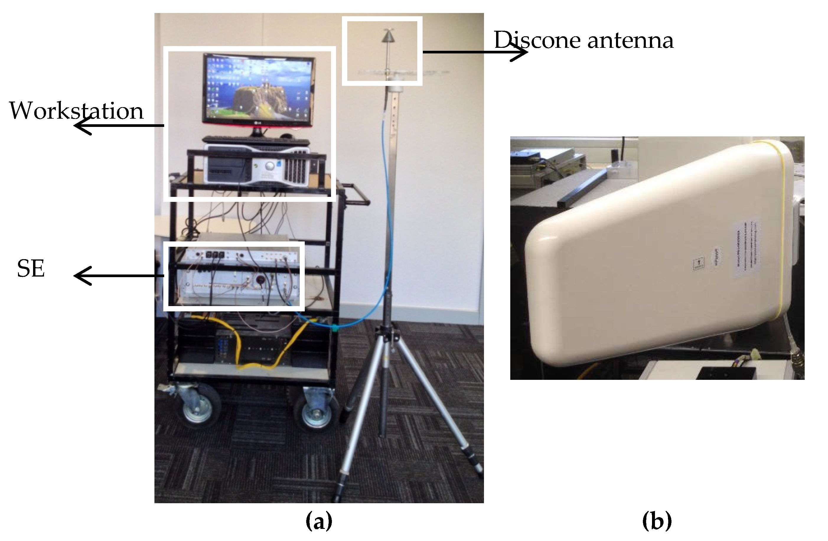
To analyze the occupancy of the 2.4 GHz WLAN signal, the bandwidth of the SE was configured to 100 MHz centered at 2.45 GHz with a time resolution of 204.8 µsec. A custom-designed wideband omni-directional discone antenna, placed at 1.5 m above ground, as shown in
Figure 2a, was used in the measurements. The measurements were taken during working hours from 01:15 pm to 01:35 pm in an indoor environment. For the directional measurements, three commercial log periodic vertically-polarized antennae (see
Figure 2b) were used with beam widths of 55 degrees. The antennae were placed at 1.5 m above ground with an angular separation of 90 degrees. Due to having three antennae, switching at 204.8 µsec, the time resolution per antenna or angle was 819.2 µsec, which corresponds to the switching time between three antennae, and an additional reference sweep was taken to get the correct antenna switching sequence in each data file. The measurements were performed in the same environment from 05:20 pm to 05:40 pm.
At the beginning of each measurement, the radio frequency (RF) attenuator and signal conditioning (SC) gains were calculated based on the sampled data and recorded to calibrate the received power. In both sets of measurements, the raw data were acquired with an 80 MHz sampling rate in multiple files where each file contains 2 seconds of data. Over 976,000 snapshots were collected for both omni-directional and directional setups and processed with 400 kHz frequency resolution by applying a high-order Gaussian window which is sufficient to detect 2.4 GHz WLAN signals or any other available short duration signals in the 2.4 GHz ISM band.
4. Data Analysis Methodology
To estimate the detection of signals in the sensed bandwidth, the energy detection [
28] approach was used where the received power was compared with a predefined threshold to define the state of the channel. A channel was considered in a busy state if the received power was above the predefined threshold and otherwise considered in the idle state. Based on this, a binary time series was created in which ‘1’ represents the busy state (presence of signal) and ‘0’ represents the idle state (absence of signal). To find the spectrum utilization, the duty cycle (DC) was calculated based on the binary time series using Equation (1):
The DC is an important parameter and its lower values indicate the availability of the ITWs.
The duration of consecutive 0’s i.e., ITW, in the binary time series was computed along with its empirical cumulative distribution function (CDF). The empirical distribution was fitted with GP, WB, EX, GM and LN distributions. The associated parameters (shape: k, scale: δ and location: µ) were found based on the maximum likelihood techniques and used to compute the mean (M) for the fitted distribution.
Table 3 summarizes the distribution functions along with the mean formula for the respective distribution.
To measure the goodness of fit between the empirical and used distributions, Kolmogorov Smirnov (KS) test was used, and the distribution with minimum KS distance was chosen as the best representative of the empirical distribution.
5. Omni-Directional Antenna Measurements
This section provides analysis of the measurements taken with the omni-directional antenna.
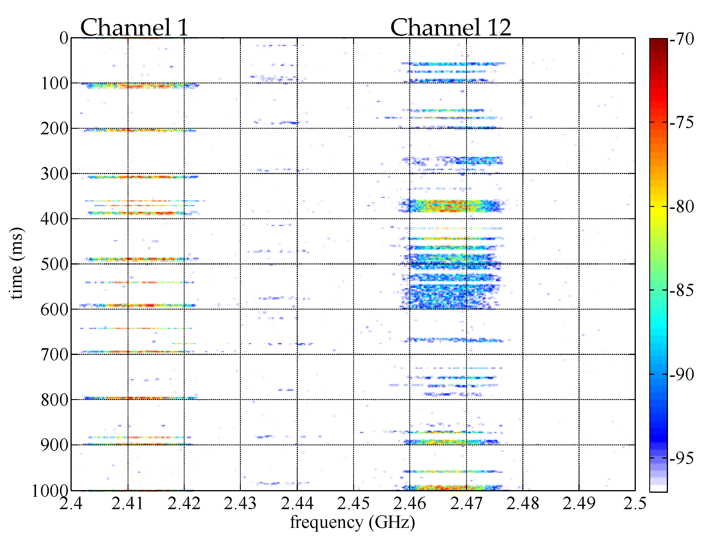
Figure 3 displays the time-frequency map of the WLAN traffic over the duration of 1 second, where −97 dBm is chosen as the decision threshold which is 10 dB above the measured noise floor and found to be the noise-free region.
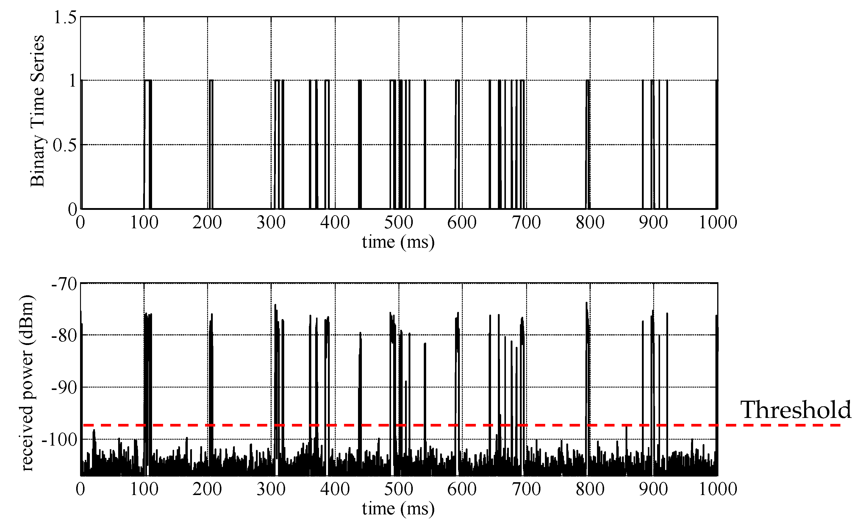
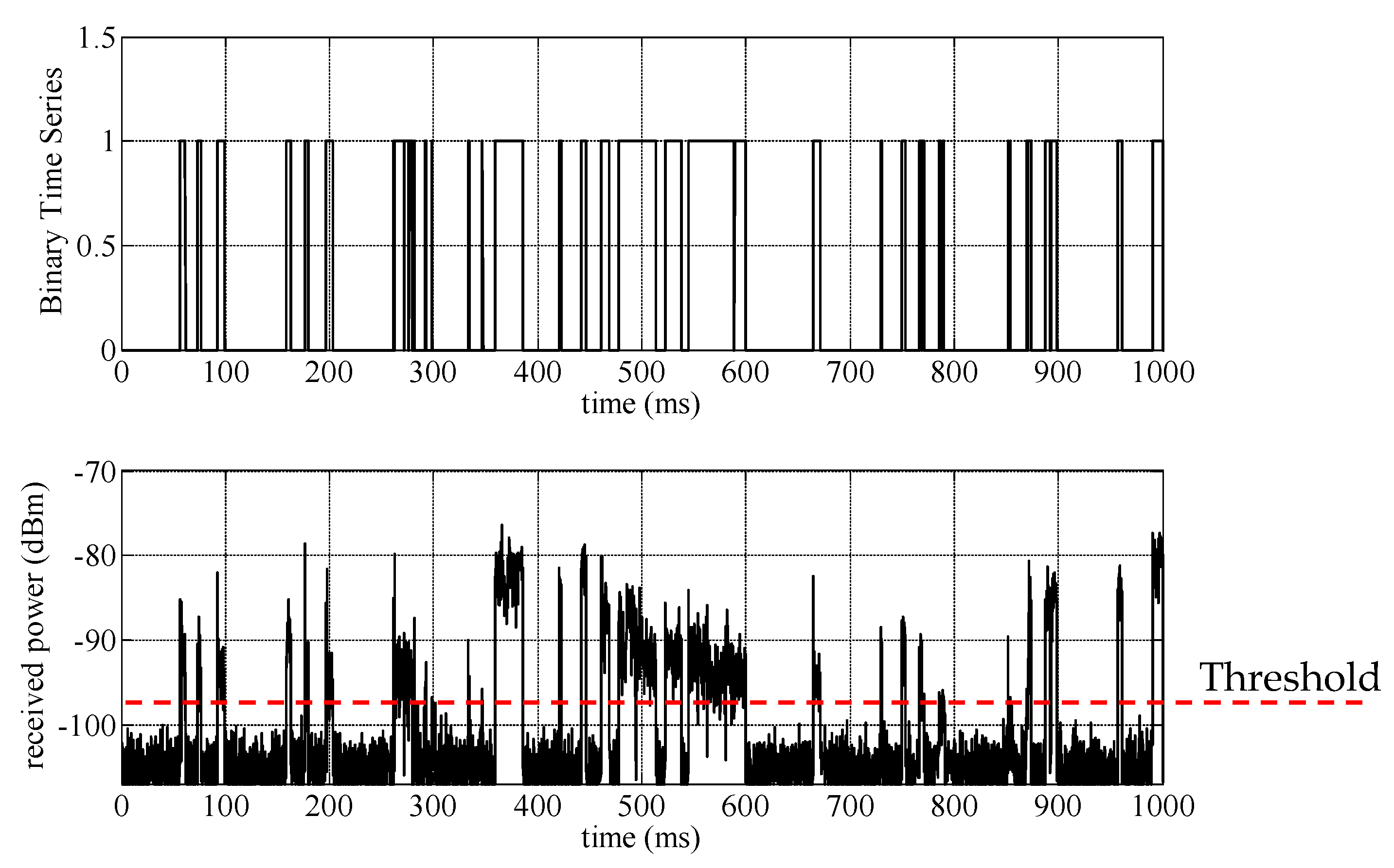
Figure 3 shows that most of the users’ activity was present in the WLAN channels ‘1’ and ‘12’. There are different WLAN packets with different durations. For example, channel ‘1’ did not remain in the busy state all the time. It remains in the idle state for various durations as represented by the ‘white’ color in the time-frequency map. Thus, by exploiting the idle state of the channel it can be accessed in the time domain by CR users. To find the statistics of the ITW, both channels were further processed to get the binary time series as shown in
Figure 4 and
Figure 5. Based on the binary time series, the DC values were found to be 7.4013% in channel ‘1‘, 11.5071% in channel ‘12‘ and 4.6449% over full-sensed bandwidth. These lower DC values indicate that both channels are highly underutilized and can be used for opportunistic spectrum access.
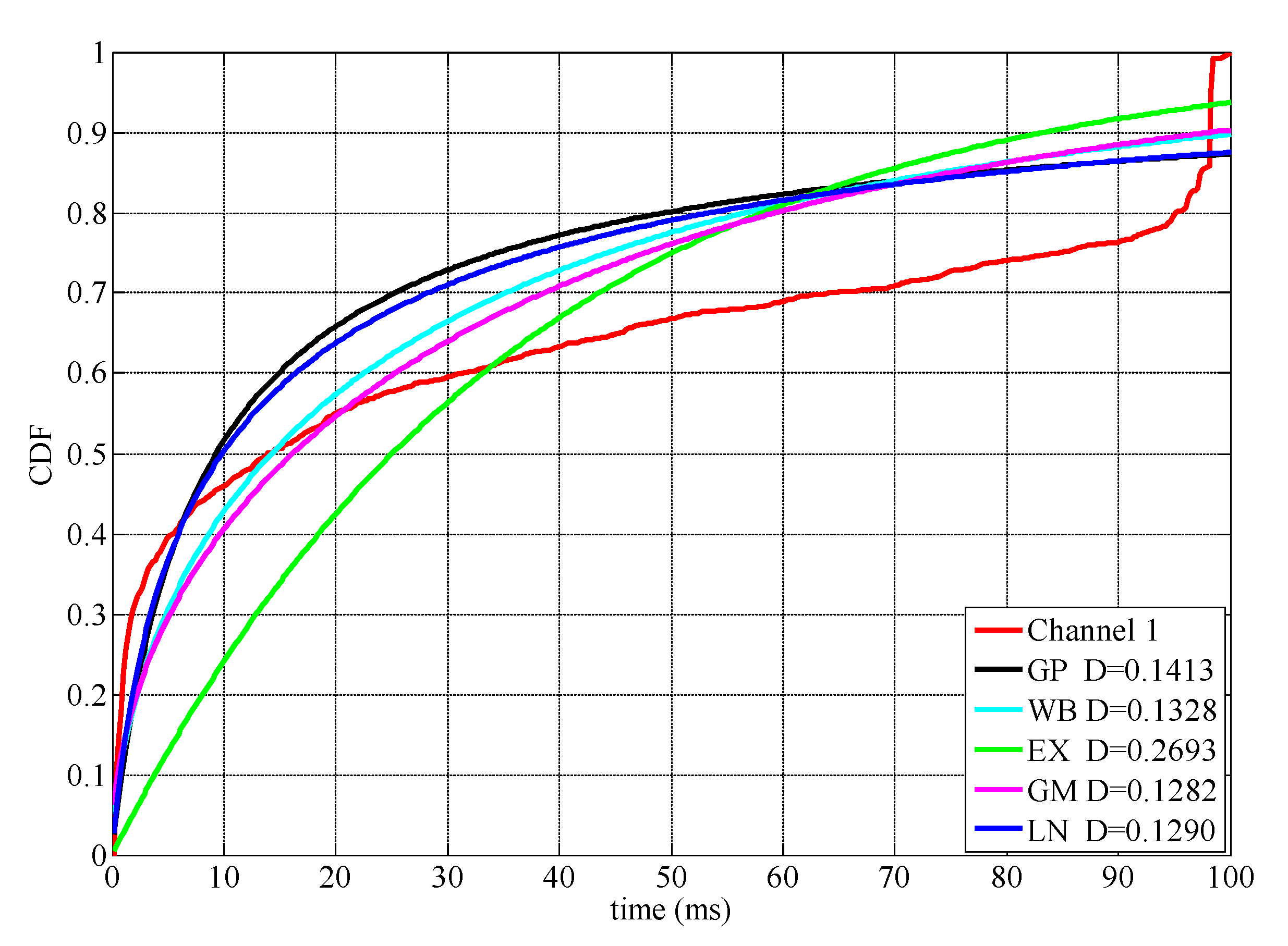
Figure 6 shows the empirical CDF of the ITW found in channel ‘1’. The gamma distribution provides the best fit with minimum KS distance. The estimated parameters are k = 0.4898, δ = 73.8318 and the mean M = 36.1628 ms. Apart from this, the log normal distribution also provides the second best fit. It is also important to observe that the empirical CDF tends to increase rapidly in the interval (95 ms to 100 ms). The reason for such long windows is because the channel was in the idle state most of the time and the occupancy state was changing due to the arrival of the beacon packet which was observed every 100 ms.
Figure 4 also shows that the beacon packets were detected at t = 0, 100, 200 and 800 ms.
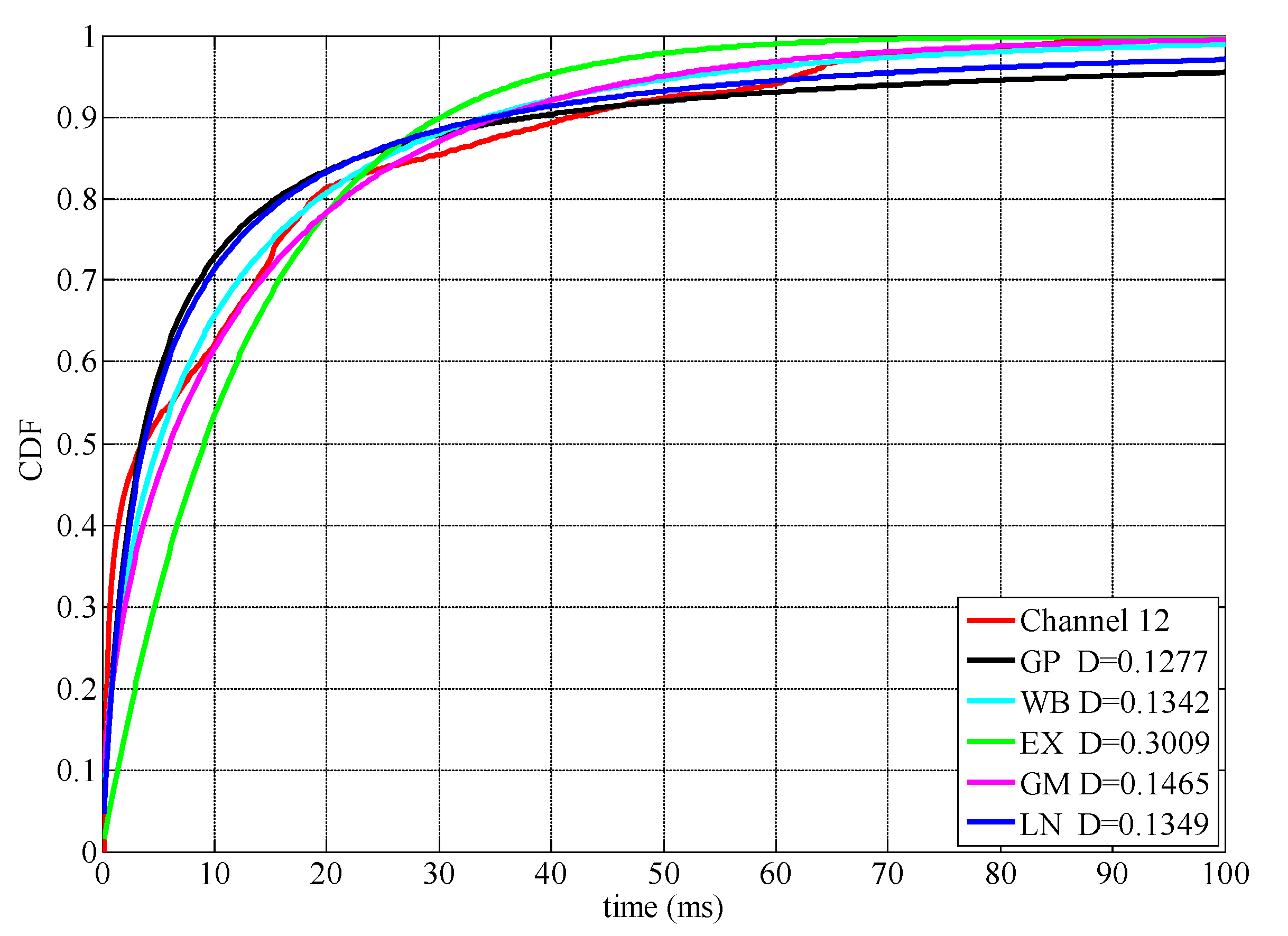
Figure 7 shows the empirical CDF of the ITW in channel ‘12’ where the GP distribution provides the best fit with estimated parameters k = 1.1620 and δ = 3.285. Although it provides the best fit, since k > 1, the mean of the distribution is not finite. To calculate the mean value, the WB distribution parameters are used, which provide the second best fit to the empirical CDF. The estimated parameters for this distribution are k = 0.6255 and δ = 9.0156 and the mean M = 12.8766 ms. By comparing both empirical CDFs, it is observed that channel ‘1’ has less traffic load which provides longer ITW, so it is most suitable for CR users. Another key observation is that, it is not possible to have ITW longer than 100 ms since the WLAN access point was periodically transmitting a beacon packet approximately every 100 ms.
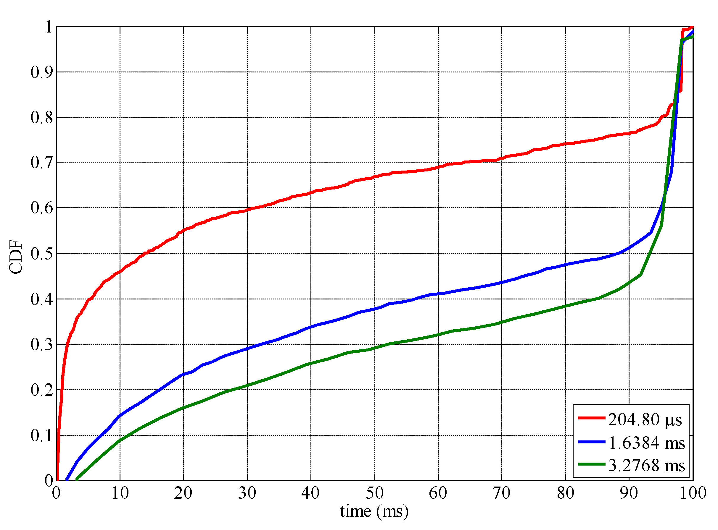
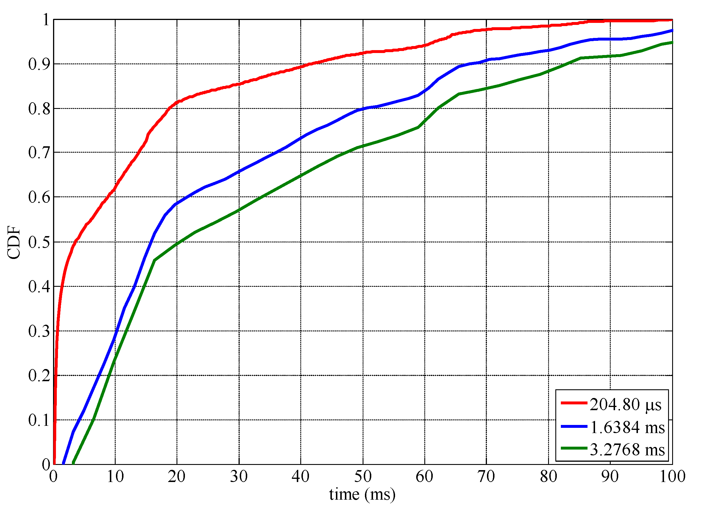
Since the SE uses a frequency sweep, each frequency point was traversed after the configured time resolution. To investigate the effect of low time resolution on the statistics of ITW, the time series of both channels were resampled individually in the time domain with 1.6384 ms and 3.2768 ms time resolutions. This illustrates the effect on the ITW when the network traffic is sensed using a low time resolution SE.
Figure 8 and
Figure 9 show the effect of different time resolutions on channels ‘1’ and ‘12’, where reducing the time resolution tends to increase the duration of the ITW. This apparent increase is due to the SE inability to detect packets with a duration less than the time resolution. Thus, measurements performed using low time resolution SE do not provide reliable data for modelling time-based opportunistic spectrum access.
The empirical distributions can be further utilized to study how the variability of the load in a channel affects the fitted distributions and their parameters.
Table 4 summarizes the KS distance between the empirical and fitted distributions (best distributions are marked bold). The GP distribution is found to have the best fit for channel ‘1’ while the LN distribution provides the best fit for channel ‘12’ for time resolutions of 1.6384 ms and 3.2768 ms, respectively.
For both channels, the mean ITW were calculated for comparison.
Table 5 summarizes the parameters and the mean value for the distributions which provided the best fit. The mean value tends to increase with the drop in traffic load as the channels remain in the idle state for longer time windows. These results show that in previous work [
20,
24], where the GP distribution was shown to provide the second best fit, the LN and GM distributions can also be used to model the behavior of the ITW for different network traffic loads. Moreover, by having wideband detection capability, a CR user can monitor the traffic load on particular or multiple channels and can concurrently exploit the idle states in multiple channels or radio technologies (e.g., 2.4 GHz WLAN and Bluetooth).
6. Directional Measurements
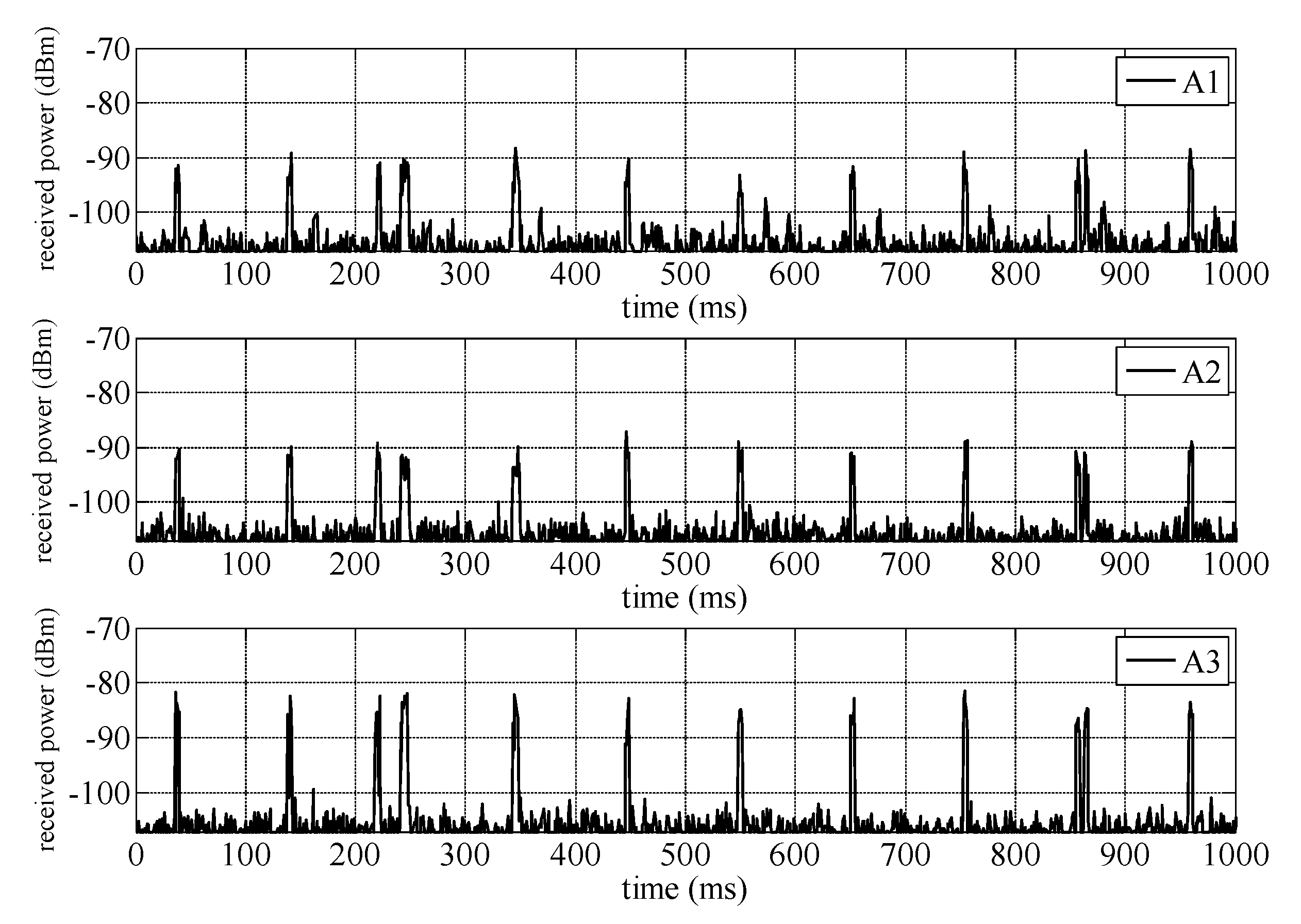
The influence of the angle of arrival on the statistics of the ITW is studied from directional measurements. Three antennae (A1, A2 and A3) were used for this indoor measurement.
Figure 10 shows the effect of different directions on the received power in channel ‘1’ where it can be observed that antenna A3 has a higher received power compared to the other two antennae. Similarly, antenna A1 has a higher received power for channel ‘12’ as shown in
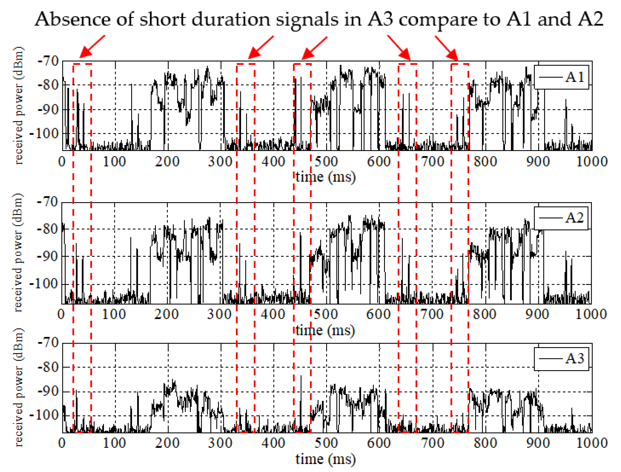
Figure 11. While it is expected that the signal power varies with the angle of arrival, if at a certain direction the received power is lower than the decision threshold due to propagation losses, the channel may be considered in the idle state. Further to this, the time resolution per antenna also affects the state of the channel. For example, consider channel ‘12’ on antenna A3, where the received power dropped by more than 10 dB and it could no longer detect short duration signals.
A decision threshold of −97 dBm, 10 dB above the measured noise floor, was used per direction to find the respective binary time series.
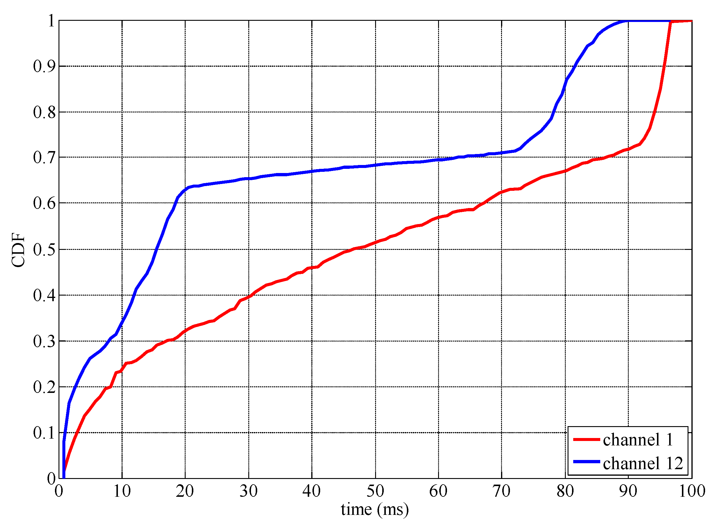
Table 6 compares the DC values in relation to different directional antennas and gives a summary of the DC values based on the omni-directional antenna. To remove the uncertainty in the occupancy state due to the variation in the received power or the effect of time resolution per antenna, the binary time series were combined using the OR hard combining data fusion technique, where a channel is considered in the busy state if it is detected in any direction. This series is used to compute the empirical CDF of the ITW.
Figure 12 shows the empirical CDF of both channels and
Table 7 summarizes the KS distance for fitted distributions (best distributions are marked in bold). The Weibull distribution provides the best fit for channel ‘1’ with parameters k = 1.1070, δ = 51.7498 and M = 49.8307 ms. Channel ‘12’ empirical CDF is fitted best with the lognormal distribution with parameters δ = 1.4980, µ = 2.6644 and M = 44.0975 ms. Thus, the analysis shows that the angular dimension can influence the statistics of the idle window due to propagation losses and the time resolution per antenna used to acquire the data. To compensate for these effects, decisions can be made using the OR-combining technique. However, the time domain-based directional opportunistic spectrum access can be vital in cases where communication links of licensed users are highly directional.
The opportunistic spectrum access will play an important role in future wireless networks like Internet of Things, device-to-device, 5G, and drones assisted, to improve spectrum utilization and overcome the spectrum demands from emerging applications in smart cities, connected health and retail sector, to count a few. Due to the wide spread availability for 2.4 GHz WLAN signals, our work will be a step forward for unlicensed users from emerging applications to access the spectrum without causing interference. The reported set of measurements and the numerical simple distributions to model the occupancy will allow users to access the spectrum without performing periodic spectrum sensing. In addition, our findings relating the impact of time resolutions and angle of arrival will be useful to properly plan spectrum occupancy measurements and build models in other wireless communication technologies.


