Article

A Long-Range 2.4G Network System and Scheduling Scheme for Aquatic Environmental Monitoring

College of Engineering Science and Technology, Shanghai Ocean University, Shanghai 201306, China
*
Author to whom correspondence should be addressed.
Electronics 2019, 8(8), 909; https://doi.org/10.3390/electronics8080909
Submission received: 17 July 2019 / Revised: 9 August 2019 / Accepted: 14 August 2019 / Published: 17 August 2019
(This article belongs to the Section Networks)

Abstract

:
Wireless communications for applications of inshore fishery and large area aquatic environmental monitoring are really challenging, due to the characteristics of a long monitoring period, large coverage area, and adverse transmission conditions. Recently, LPWAN (low-power wide-area network) became the new solution to address these challenges, due to its long transmission distance and low power consumption of end-nodes. In this paper, we designed a novel network system for aquatic environmental monitoring, based on long-range 2.4G technology, which consisted of a low cost dual-channel gateway and end-nodes. A DMSF (dual-channel multiple spreading factors)–TDMA (time division multiple access) MAC (medium access control) scheme for this system was proposed, which largely reduces the channel collision probability, and improves the real-time for urgent data and the average lifetime of end-nodes. We verified the applicability of the long-range 2.4G technology in an aquatic environment, by point-to-point communication experiments over lake water. The performance evaluation and analysis of DMSF–TDMA is presented through simulations, and comparison with other existing schemes. The results demonstrated the benefit of our proposed scheme, in terms of the packet delivery rate, delay, and energy consumption.

1. Introduction

The Internet of Things (IoT) is emerging as a set of technologies, which refer to the inter-connection and exchange of data among devices and sensors, and has revolutionized the way people perceive environments [1]. During the last decade, with the explosive growth of the IoT technologies, an increasing number of practical applications can be found in many fields, especially in various environmental monitoring scenarios [2,3].
Due to many water pollution problems, aquatic environmental monitoring draws many an interest of researchers in recent years [4,5,6]. Aquatic environmental monitoring system with IoT technologies is not only important to monitor water quality but it could be used to provide an early warning of contaminants in the water and also to monitor fish stocks. It should meet the following requirements: Long-term deployment, large area coverage, communication reliability, real-time alarm and low cost. Aim at this application, it is obvious that the sensor nodes should be characterized by long range and low power communication, and the communication protocol must be designed to obtain the highest possible energy savings while ensuring real-time uploading of the urgent data.
Motivated by above challenges, in this paper, we consider the large area and large scale aquatic environmental monitoring scenarios, all of the end-nodes periodically transmit data to the gateway, when a critical event or abnormal data is detected, end-nodes can report urgent data to the gateway in real time so that appropriate action can be taken promptly. In such scenarios we focus on how to minimize energy consumption of the sensor nodes while achieving reliable and low-delay data transmission in long-range and low-power sensor networks. To achieve our objectives, a LoRa (long-range) 2.4G network system is designed, in which the end nodes and the dual-channel gateway use the LoRa 2.4G transceiver; a DMSF (dual-channel multiple spreading Factor)-TDMA (time division multiple access) MAC (medium access control) scheme for this system is present, which is built on LoRa 2.4G MAC layer and combines improved TDMA mechanism with adaptive SFs (spreading factors) based on link quality, for aquatic environmental monitoring.
The subsequent sections of this paper are organized as follows. In Section 2, we introduce some related work. In Section 3, we test the communication performance of LoRa 2.4G transceiver for aquatic environmental monitoring. Then, in Section 4, a LoRa 2.4G network system and a DMSF–TDMA scheme for the MAC layer is present in detail. Section 5 gives the simulations, analyses and implementation results for the proposed scheme. Finally, Section 6 concludes the paper and mentions the future work.

2. Related Work

In this section, we present the related work of wireless communication technologies for aquatic environmental monitoring in recent years. We also give the properties of our scheme, which differ from previous work at the end of the section.
Many researchers adopted short-range communication technologies, such as ZigBee, to monitor aquatic environment [6,7,8,9]. The common architecture of these applications is present in [9], which consists of sensor nodes, sink nodes, and a server. Sensor nodes can sense environmental parameters such as water temperature, salinity, pH, oxygen density, etc., and transmit the sensing data to sink nodes by Zigbee WSN. A sink node collects data from sensor nodes in local network, and transmits the collected data to the server by the Internet.
ZigBee uses the IEEE 802.15.4 physical and data link layers, which enables low-cost and low power transceivers, but suffers from a range of only a few tens of meters. In work [10], the wireless module on the sensor node integrates a power amplifier for the transceiver to allow the transmission distance over 1 km, at the cost of minimum transmission power of 20 dBm.
ZigBee can expand the network coverage by multi-hop communication. However, its disadvantages are at the cost of higher latency and higher power consumptions. Although many low-power MAC protocols for IEEE 802.15.4 transceivers are proposed to reduce the energy consumptions [11], with the increase of hops, the end-to-end delay and management complexity increases, and communication reliability decreases [12].
Some researchers propose cluster topology for aquatic environment monitoring, which used IEEE 802.15.4 transceivers for cluster communication [13,14]. In work [13], the cluster head (gateway) is equipped with a long-range 2.4GHz module, which allows remote transmission (up to 16 km) to the base station. The power consumption of the cluster head module is particularly high (being around 0.75 W in transmission), therefore it is equipped with a solar panel for energy harvesting, and a modified TDMA schedule mechanism is present to improve the energy efficiency. In work [14,15,16,17], the cluster head is equipped with a GPRS (general packet radio service) module that can provide a longer range. In work [18,19], the sensor node directly uses the GSM/GPRS modem for long-range communication. However, the GPRS module has higher power consumption and operating costs, and the network coverage and capability depend on the existing infrastructure.
LPWAN represents a new trend in the evolution of IoT technologies. In contrast to cellular network (GPRS, 4G, and 5G) or WiFi, the high data rate for end-nodes is not the design factor firstly considered. Instead, the data rate in LPWAN is intentionally traded off for the long transmission distance. The key performance metrics defined for LPWAN are energy efficiency, scalability, and coverage [20,21].
Among existing LPWAN technologies, LoRa is one of the most prominent and receiving great attention from researchers. Due to the utilization of unlicensed bands, LoRa technology is perfect for outlying regions without cellular network coverage, and for establishing private networks with specific requirements for quality and security [22].
LoRa has been very successful in the market due to its open protocol standard and chirp spread spectrum (CSS) modulation technique that allows recovering data from weak signals even below the noise floor. Due to this technique, it has long-range characteristics while maintaining robustness to interference, and is inherently secure. To control the trade-off between the transmission range and data rate, LoRa allows configuring the radios with different orthogonal spreading factors (SFs). A higher SF increases receiver sensitivity and thus range, but decreases the symbol rate. Since the different SFs’ signals are orthogonal, the simultaneous transmission in the same frequency channel using different SFs is possible [23].
LoRaWAN, the MAC protocol built on the LoRa physical layer, is ideal for applications with low-traffic and sporadic communication requirements. A LoRaWAN network is based on a star-of-stars topology composed of three basic elements: End-nodes, gateways, and a central network server. One of the attractive features is its energy efficiency for uplink communication while achieving a long range. In LoRaWAN, the distributed battery-operated end-nodes send data directly to an always-on gateway. The energy efficiency comes by duty-cycling the transceiver of end-nodes when not transmitting [24,25,26].
Due to its advantages, interesting applications for maritime scenarios are already being introduced based on LoRa/LoRaWAN [27,28,29,30]. The work in [27] presented a LoRa-based sailing monitoring system, the performance of coverage and packet loss rate in the sea area was evaluated by the LoRa transmission experiment with SF9. Similar experiments were also conducted in [28], but with SF12, so obtained the further communication range. In work [29], a boat tracking and monitoring system based on LoRa was also present, the work study the link-reliability, transmission range and coverage in maritime scenarios, by point-to-point LoRa communication experiments with more LoRa setting parameters. The authors of [30] investigated the LoRa links over seawater in two scenarios: Clear line-of-sight (LOS) and obstructed path, with different LoRa devices and different LoRa parameters, and explored short and long-term variability in terms of RSS, SNR, and packet delivery ratio (PDR) in detail. All these works showed the good coverage performance of LoRa technology in maritime scenarios, however, the scalability of LoRa networks in these applications is not analyzed.
Although LoRa/LoRaWAN is gaining popularity, it still faces several challenges for environmental monitoring. The works in [26,31] show that the PDR of uplink traffic decreases exponentially with the network size in LoRaWAN. The LoRaWAN duty-cycle-based medium access control (MAC) scheme may increase packet collision probability and delay [32]. LoRaWAN is based on the ALOHA access of the channel. Without any information about neighbors or their transmission schedule, data transmission by more than one node at the same time may result in data collision. Even though the communication requirements can be low-traffic, a great quantity of high-density end-nodes trying to access the wireless channel simultaneously can be unmanageable by pure ALOHA [33]. These limitations are becoming a serious bottleneck for large-scale deployment, especially when high SFs are used. Using a higher SF can significantly extend the communication range by increasing the receiver sensitivity, but the drawback is that doing so can cause more severe data collision due to the longer transmission time on air.
Therefore, some authors proposed to synchronize the LoRa network [26,33]. RS-LoRa MAC proposed in [26] divides the available bandwidth into single synchronous downlink channel and several asynchronous uplink/downlink channels, through lightweight scheduling, based on the received signal strength at both nodes and gateways. It improves the reliability and scalability of LoRaWAN, but does not consider the delay of urgent data. The authors of [33] present energy-efficient network architecture and a high-efficiency TDMA protocol for LoRa networks to improve both the energy efficiency and the latency, at the cost of installing an additional wake-up receiver on each LoRa node.
In work [34], an adapted CSMA (carrier sense multiple access) mechanism for LoRa networks is proposed to avoid costly packet collision. The authors of [35] propose a CSMA/CCA algorithm to deal with the collision problem to enable reliable multiparty communication. L-MAC proposed in [36] reuses beacon messages of receiver initiated MAC protocols to enable nodes to coordinate their wakeup time with their parent nodes, and the inter-branch, intra-branch, and inter-flow collision avoidance solutions are present. The CSMA-like mechanisms in these works can be used for reference to relieve the risk of collision in LoRa networks.
In 2017, Semtech introduced new long-range 2.4 GHz wireless RF technology and transceiver SX1280, which enables long-range, scalable data rate communication for point-to-point wireless links, and complements existing wireless technologies, such as Wi-Fi, Bluetooth, Zigbee, and LoRa. The SX1280 transceiver can support custom protocols with configurable raw data rates up to 253 kb/s by the LoRa modem in the 2.4 GHz (industrial, scientific, and medical (ISM)) band, depicted in Table 1 [37], with the linearity to withstand heavy interference. This makes them the ideal solution for robust and reliable wireless solutions. Meanwhile, it can achieve point-to-point, multipoint, multi-multipoint transparent data transfer between devices. Furthermore, the devices that communicate with each other form the network of a star.
Table 2 summarizes the typical transceiver parameters, which show the ultra-low current consumption of SX1280 at high data rate, compared with other IoT communication technologies. Although the receiver sensitivity of SX1280 is a little weaker than that of SX1278, which means the maximum transmitting distance of SX1280 is a little shorter than that of SX1278 with the same transmitting power. The high date rate means low time on air of the packet, which is conducive to reduce energy consumption of packet transmission and the probability of channel collision and increase the traffic under a given duty-cycle.
Through the above comparison, we selected LoRa 2.4 GHz technology and a transceiver for aquatic environmental monitoring. There was no special LoRa 2.4 GHz concentrator chip for gateway like SX1301, which could simultaneously receive eight LoRa packets on eight different channels using random spreading factors. The SX1301 gateway was used for LoRaWAN, the cost of which was more than a hundred euro, and the LoRaWAN protocol only supports the Sub-G band. Thus, a proper LoRa 2.4G network system and communication scheme should be proposed. Aquatic environmental monitoring is based on gathering information from end-nodes. The amount of generated data will be increased as the number of end-nodes grows. Thus, the network may experience a bottleneck at the gateway, which will drop the transmission efficiency, and the urgent data may not be uploaded in time. Therefore, the network system and communication scheme should allow for improving the reliability and delay and reduce energy consumption.
Some properties of our work that differ from the previous ones were summarized as follows:
(1) A low cost dual-channel LoRa 2.4G gateway with two SX1280 transceivers and network architecture for aquatic environmental monitoring were designed.
(2) We carried out LoRa 2.4G communication experiments with different parameters over water surface in the line-of-sight (LOS), obstructed LOS, and NLOS scenarios, to verify the applicability of such technology in aquatic environment, which are rarely implemented in other works.
(3) A DMSF–TDMA MAC scheme was present, which was based on a dual-channel gateway. One channel was used for regular packets, the scheme of which combines improved TDMA mechanism with adaptive SFs. The other channel was used for urgent data and some special functions with the orthogonal SF. It considers energy efficiency while reducing channel collision and delay in the context of aquatic environmental monitoring.

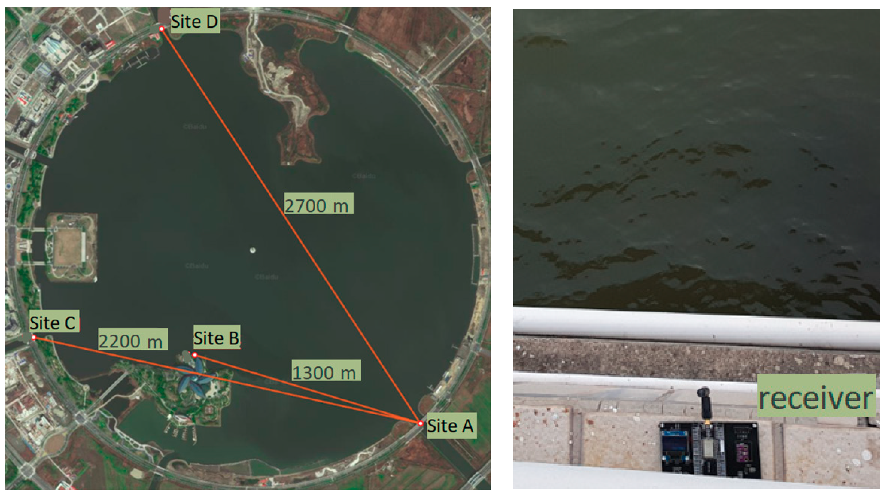
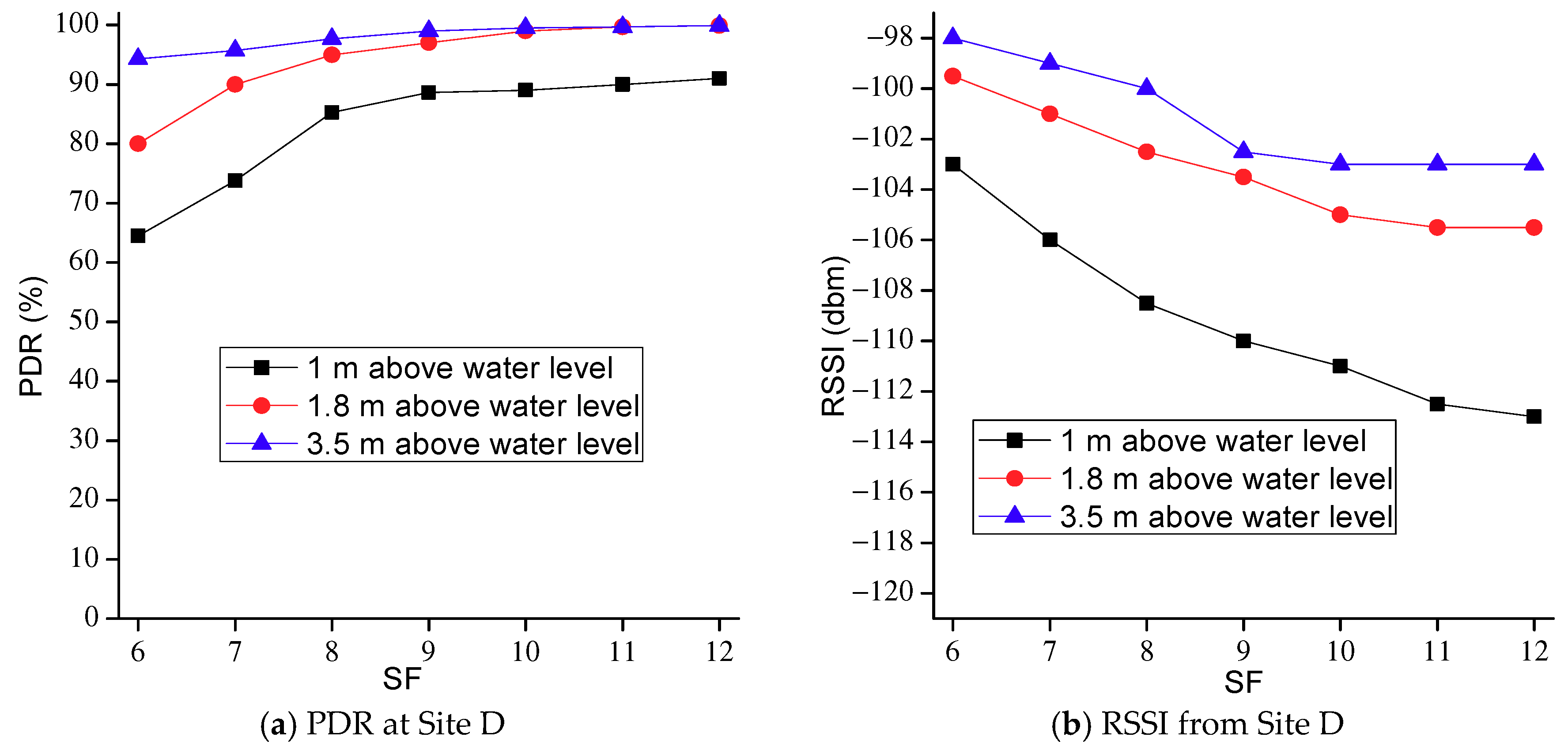
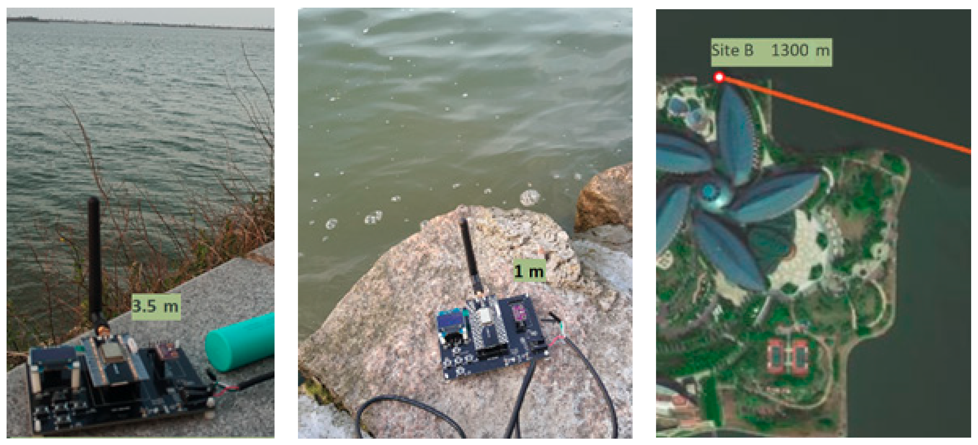
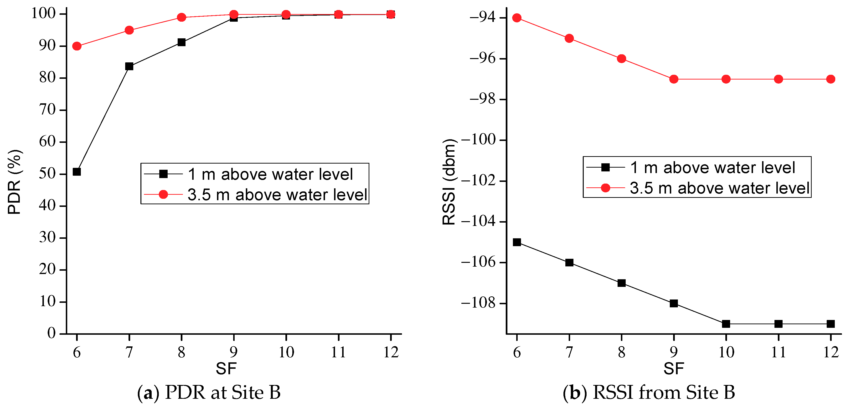
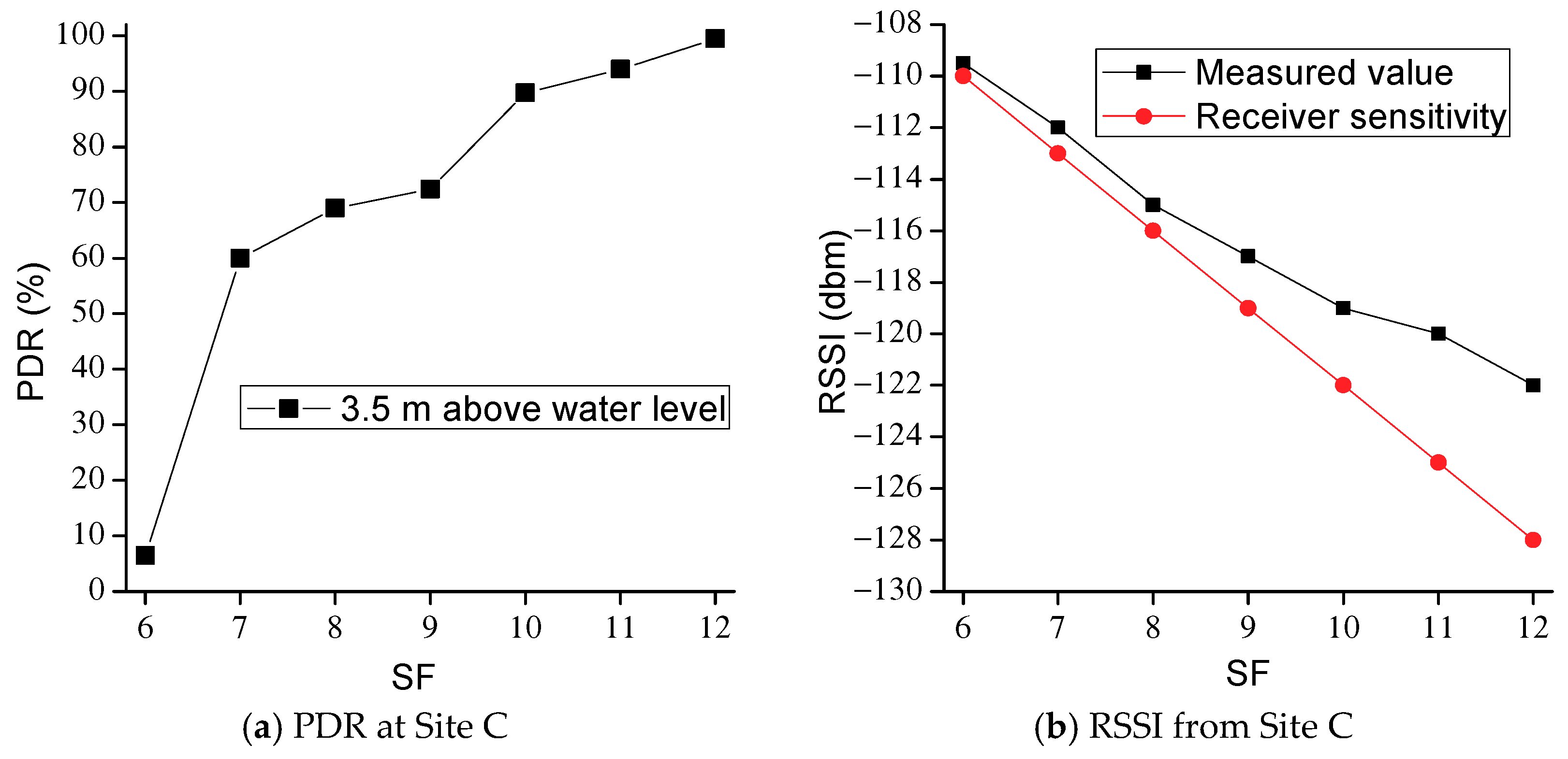
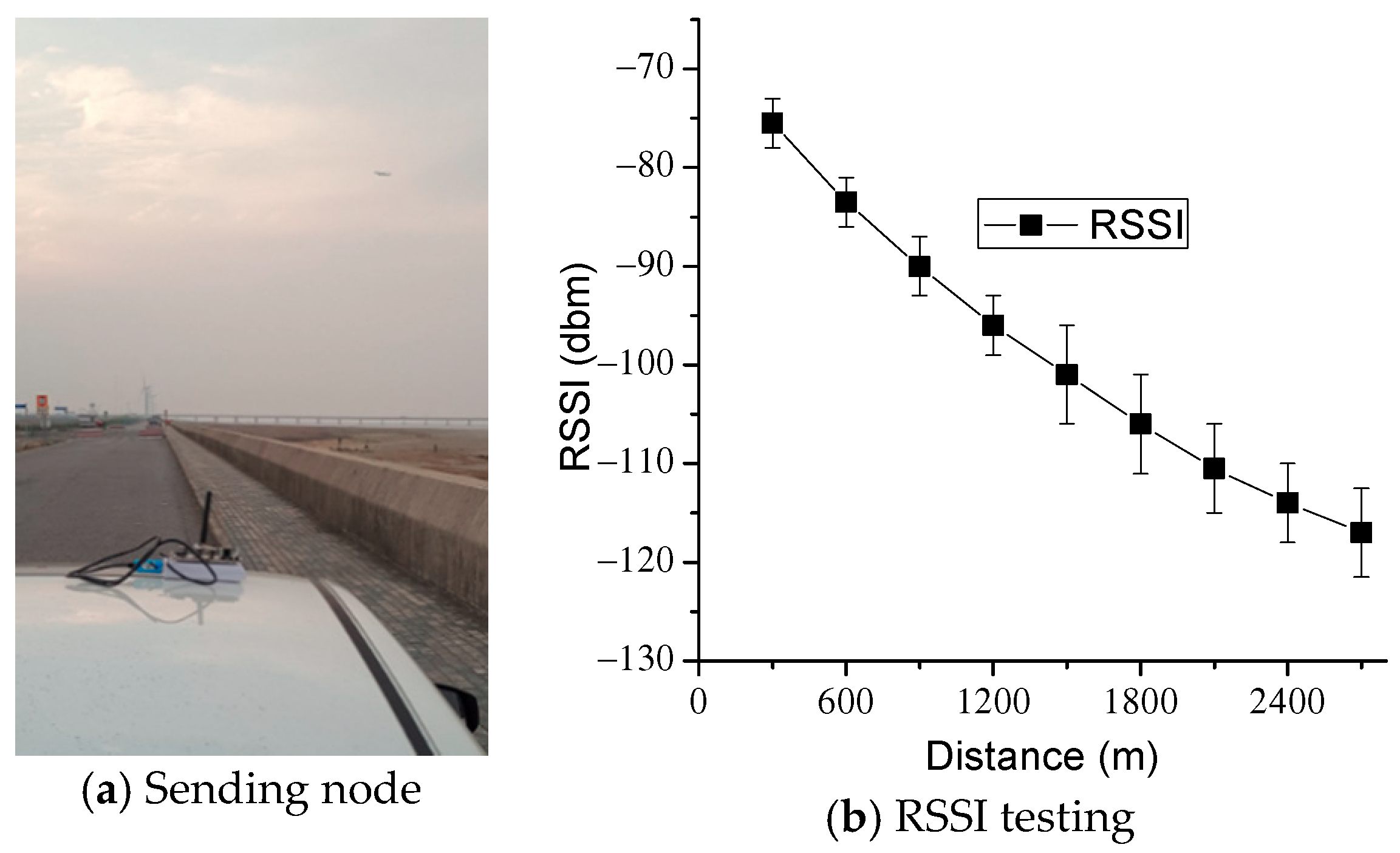
3. Experiments of LoRa 2.4G

In this section, we firstly studied the LoRa 2.4G transmitting performance by point-to-point communication experiments to verify the applicability of such technology in an aquatic environment.
All tests were implemented in the 5.6 km² Dishui Lake area in Shanghai, which is located at the sea shore. We investigated LoRa 2.4G communication performance over lake water in three characteristic scenarios: LOS, obstructed LOS, and NLOS with the different sets of LoRa parameters. The receiver node was deployed on the guardrail of bridge at Site A during all experiments, where it was 4 m above the water level, as shown in Figure 1.
The low-cost and off-the-shelf SX1280 modules and rubber duck omnidirectional antennas were used, providing gains of 3 dBi for 2.4 GHz band. All tests were carried out within the fixed transmission power of 12.5 dBm, bandwidth (BW) = 406 kHz, CR (coding rate) = 4/5, and preamble length = 8 symbol, while the SF was varied from 6 to 12, application payload size was 16 bytes. No mechanisms for delivery control and automatic retransmissions were used. The effective data rates could be obtained using the SX1280 Calculator Tool available for download on www.semtech.com. For example, using SF = 12 with the above setting, the effective data rate was 0.952 kb/s, the time on the air of the packet was 406 ms; using SF = 11 with the above setting, the effective data rate was 1.74 kb/s, the time on air of the packet was 203 ms; thus using SF = 10, the time on the air of the packet was 101.5 ms. When the SF was reduced by 1, the time on air of the packet was reduced by half. Therefore, for each SF, the experiment time was different. We focused on the PDR and RSSI (received signal strength indication) in different scenarios.
The first test was conducted at site B (obstructed LOS), which was 1300 m from site A. The sending nodes were deployed on platforms 1 m and 3.5 m above water level, successively, as shown in Figure 2. The test was executed by sending 2000 packets in each round with different SFs. Figure 3 presents the average results of PDR and RSSI attained from the receiving node. It was obviously that the sending node with the higher position had the better PDR. In Figure 3a, when the sending node was deployed 3.5 m above water level, the PDR was 90%, just SF = 6; when SF > 9, the PDR was almost 100%. When the sending node was deployed 1 m above water level, the PDR dropped rapidly when SF < 9. In Figure 3b, the RSSI decreased slightly with the increase of the SF value. The reason might be that the receiver has the lower sensitivities with the lower SF, some packets below the receiving sensitivity threshold were not received.
The second test was the NLOS scenario, and the sending node was deployed at site C, which was 2200 m from site A. The test method was the same as before, because of the farther communication path with more obstacles, we only tested the case where the sending node was 3.5 m above the water surface. As could be seen in Figure 4a, the PDR decreased with the SF value, especially when SF < 10; when using SF = 6, the receiver could hardly receive packets. In Figure 4b, the RSSI almost linearly decreased with the increase of SF value, which was similar to the trend of receiver sensitivity.
The third test was the LOS scenario, and the sending node was deployed on platforms 1 m, 1.8 m, and 3.5 m above water level, successively, at site D, which was 2700 m from site A. The test results were presented in Figure 5. It could be noticed that when the sending node was deployed 1 m above water level, even setting SF = 12, the measured RSSI = −113 dbm, and the PDR was just 90%.
In fact, despite the aquatic environment being characterized by the absence of almost any obstacle, the height of the antenna over the water level also played an important role. Since the signal reflection upon water, and the reflection and diffraction may be caused by the wave ridges or moving ships, it can introduce additional signal paths.
When the sending node was deployed 1.8 m above water level, and SF > 10, the PDR was almost 100%. When the sending node was deployed 3.5 m above water level, the PDR was more than 90% for all testing SFs.
The last test measured the change of RSSI with distance in the LOS scenario, as shown in Figure 6a. The sending node was mounted on the roof of a car, and configured to SF = 12. The results were presented in Figure 6b, the average value and the standard deviation of the RSSI measured was calculated and recorded every 300 m. It was obvious that the RSSI mean dropped as the distance increased, and the standard deviation for each distance increased with the distance, but this relationship changed weakly as the distance increased. Our evaluation results show RSSI to be a promising indicator when its value was above a certain sensitivity threshold.

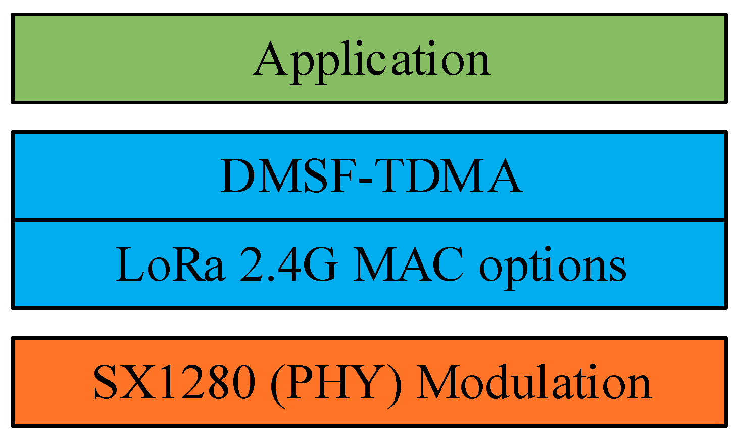
4. Network Architecture and the DMSF–TDMA Scheme

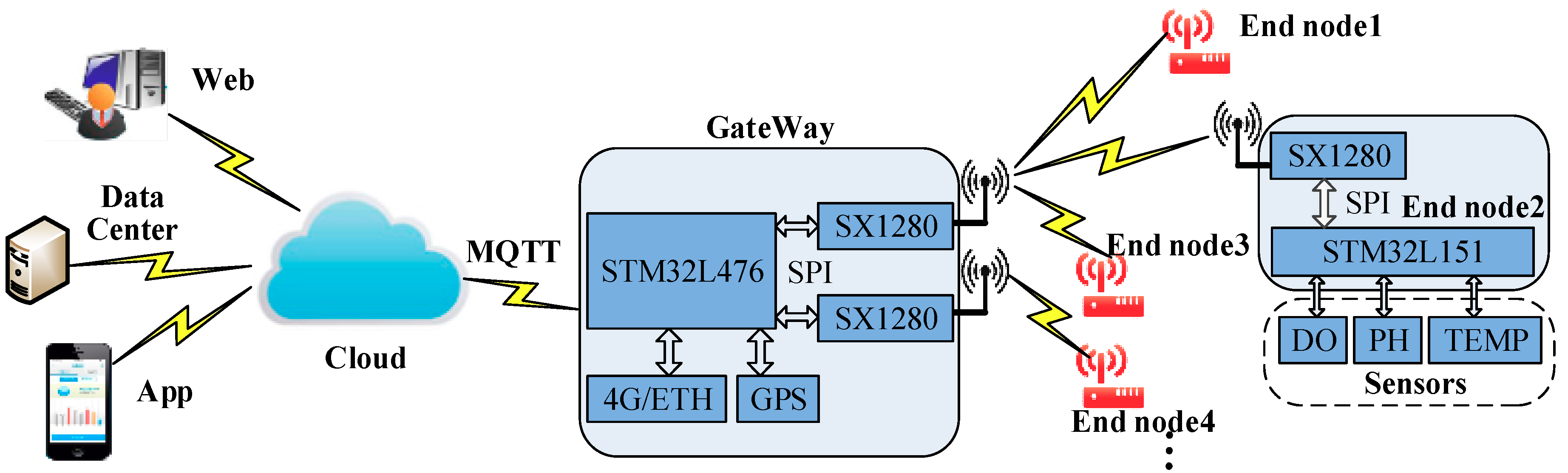
4.1. Network Architecture

Though the above experiments, we could see that LoRa 2.4 GHz technology could provide good coverage with low power in the aquatic environment. A LoRa 2.4G-to-cloud architecture was therefore proposed, in which the end-nodes transmit data to the cloud platform via the gateway, as shown in Figure 7.
The end-nodes played a key role in our proposed system, and could be powered by a battery. It mainly includes three parts: A sensor, MCU (micro controller unit), and LoRa communication unit. The sensor unit is to realize environmental parameters detection and measurement, mainly composed of the interface circuits for the sensors and the sensors themselves, i.e., dissolved oxygen (DO), pH, temperature (TEMP), conductivity, turbidity, and oxidation reduction potential (ORP). The MCU unit takes a 32-bit ARM STM32L053 microcontroller as the core, which is in charge of local decision-making and data aggregation, energy management through sleep/awake modes, etc. The STM32L053 is ST’s entry-level range of 32-bit ultra-low-power MCU designed to achieve an outstandingly low power consumption level. The exclusive combination of an Arm® Cortex®-M0 + core and STM32 ultra-low-power features, makes the STM32L053 the best fit for applications operating on batteries or supplied by energy harvesting. Its current consumption on the run mode was 88 μA/MHz, and on stop mode was 0.41 μA.
The communication unit includes the SX1280 transceiver and 2.4G antenna. The MCU uses the serial peripheral interface (SPI) to control and manage the transceiver. STM32L053 can operate read-write and issue commands to the interior registers, and access the data memory space of SX1280 to directly retrieve or write data by SPI.
We developed a low-cost LoRa 2.4 GHz gateway with two SX1280 transceivers. The gateway receives all the data from end-nodes, which forms the network of a star. It translates them into a JavaScript object notation (JSON) format, which can be uploaded to the cloud by message queue telemetry transfer (MQTT) protocol. In addition, alarm rules are defined in the IoT gateway. Once a critical event is detected, the IoT gateway will publish a message in order to notify the users.
We presented a DMSF–TDMA scheduling scheme based on LoRa 2.4 GHz technology for aquatic environmental monitoring, which aimed to improve the reliability, delay, and energy efficiency for standard LoRa 2.4 GHz networks. The protocol architecture is shown in Figure 8, the DMSF–TDMA scheme was built on the LoRa 2.4G MAC layer.

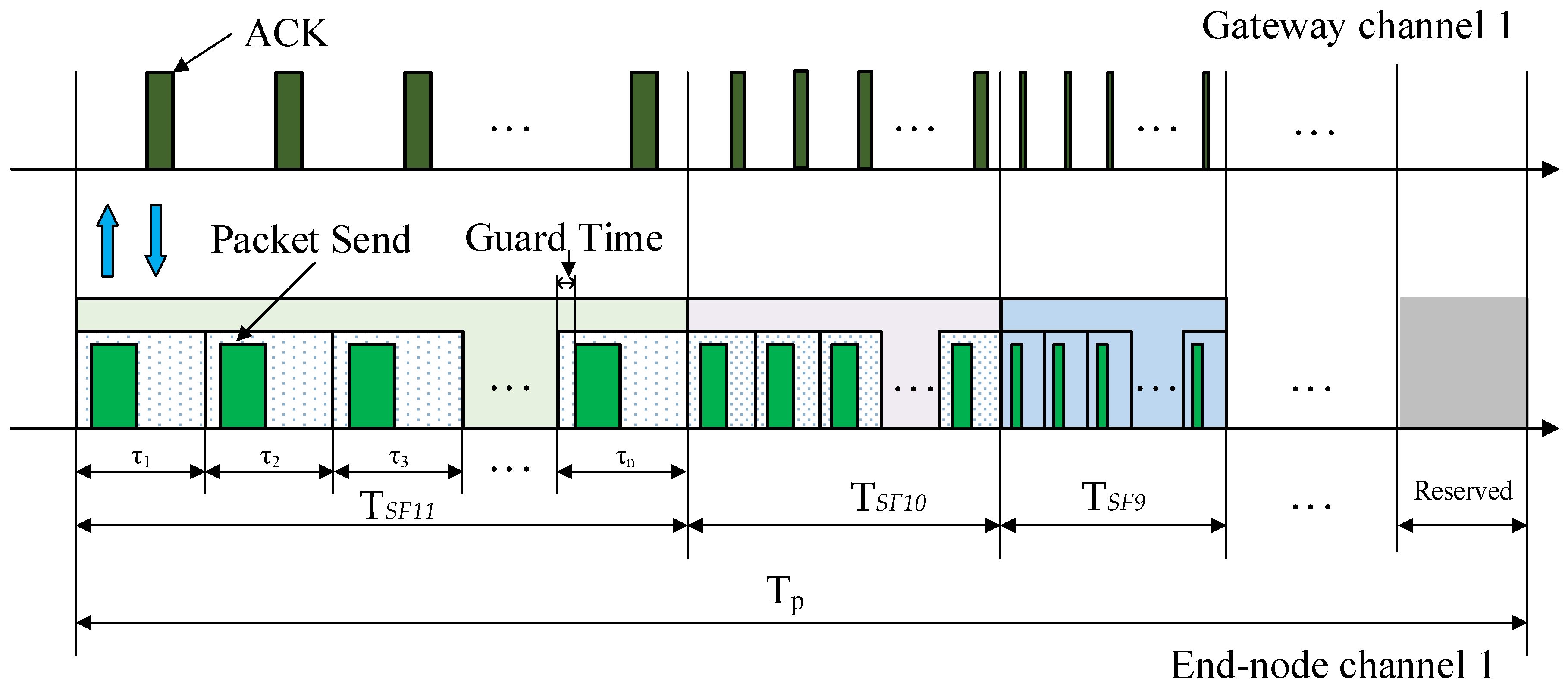
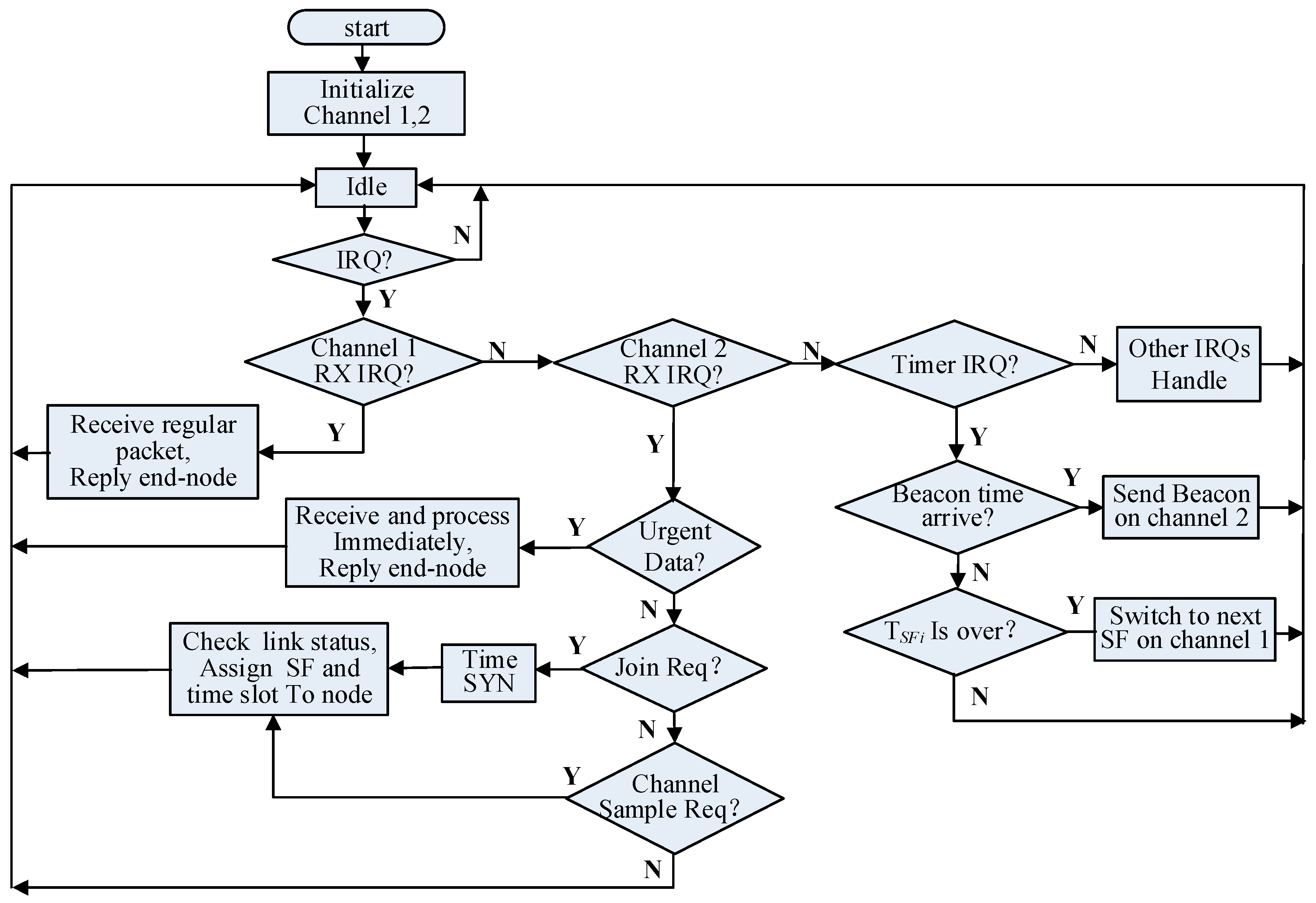
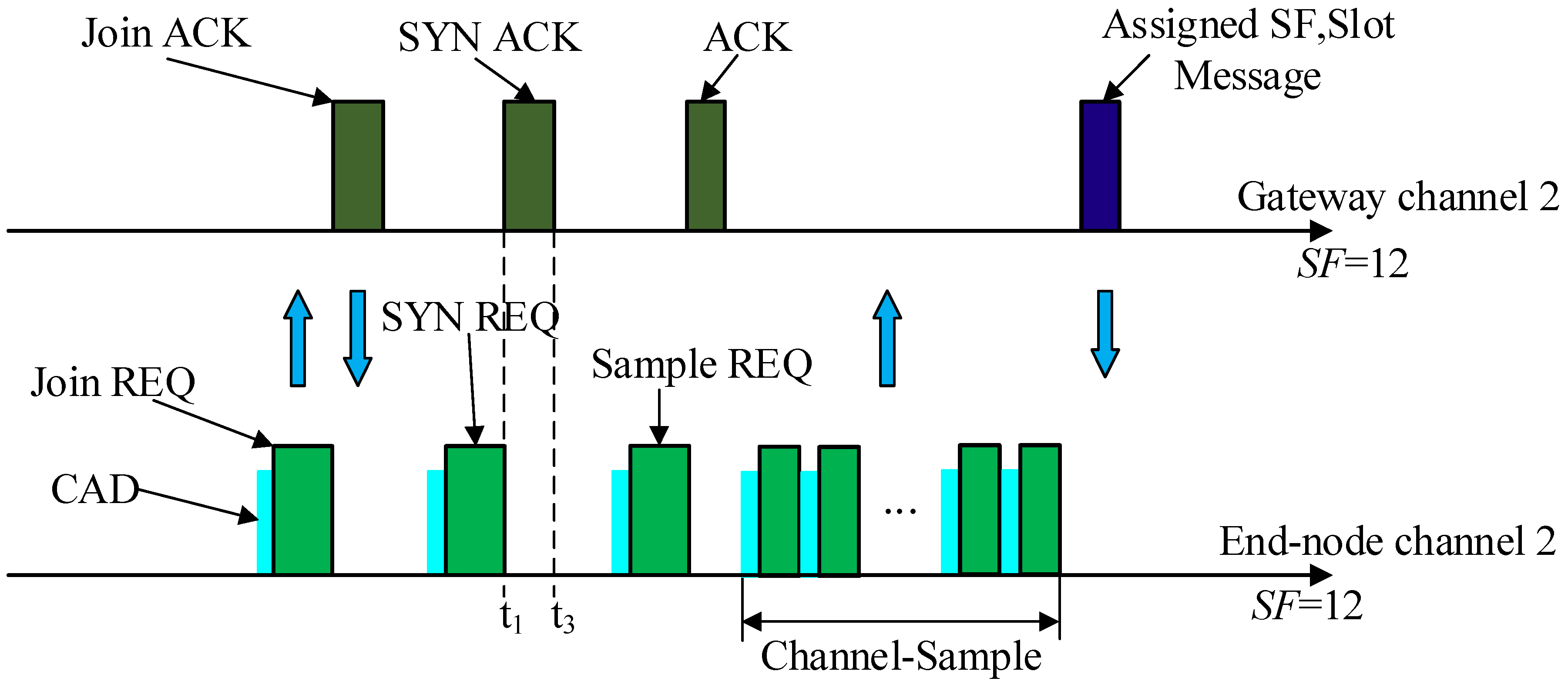
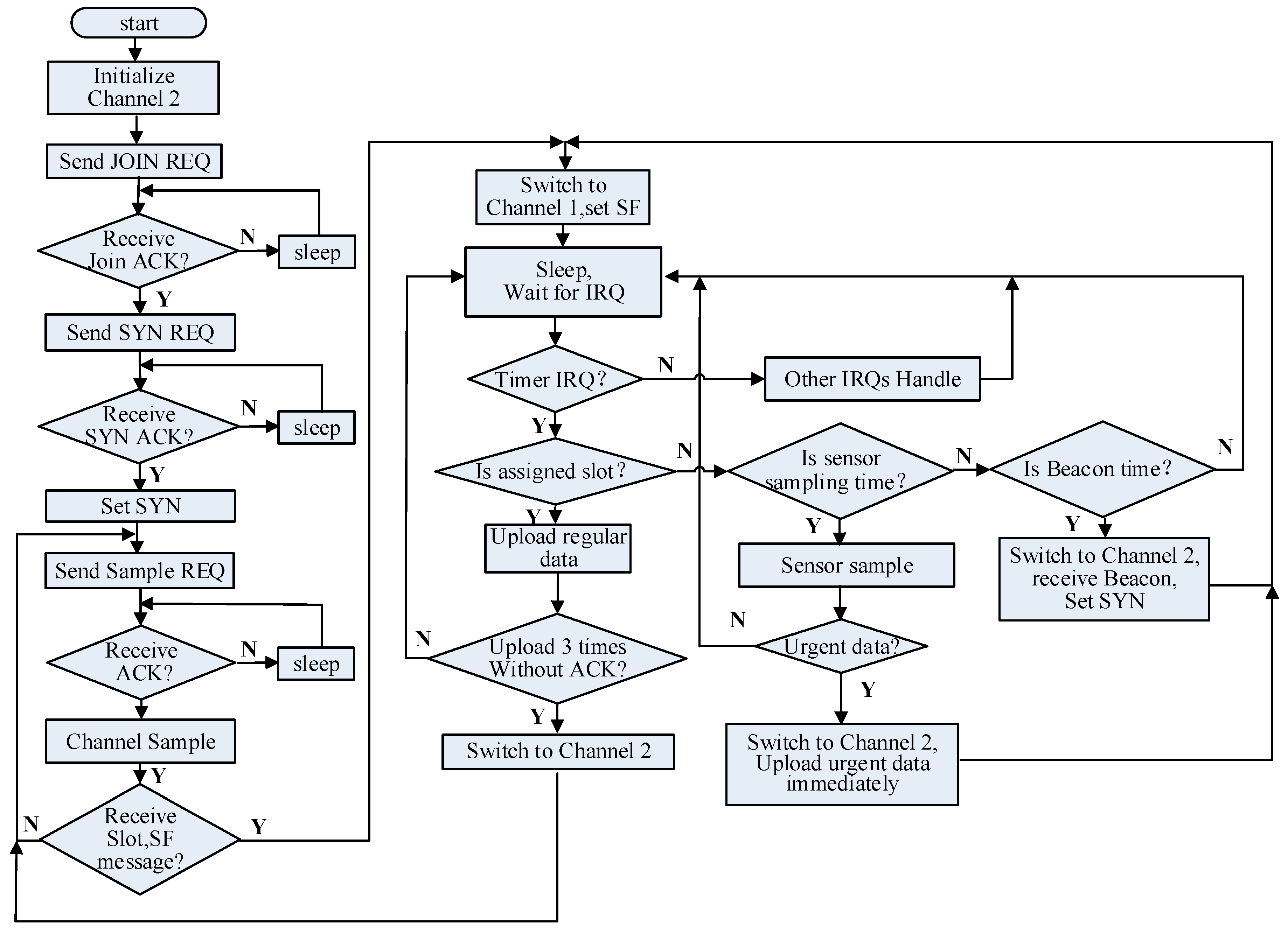
4.2. The DMSF–TDMA Scheme

In aquatic environmental monitoring system, the data packets are classified into two categories: Regular packets and urgent packets. Regular packets are used for periodic data gathering. Urgent packets are used for abnormal data and critical events. Urgent packets must be transmitted immediately when the abnormal data is measured.
Two SX1280 transceivers of the gateway provide two physical channels: Channel 1 and Channel 2. The Channel 2 has the following functions: End-nodes joining network, time synchronization, urgent packets uploading, and connectivity testing. The Channel 1 is used to transmit periodic regular packets between end-nodes and gateway.

4.2.1. Schedule of Channel 1

In DMSF–TDMA, we assumed that all end-nodes in the network transmit regular sensing data on channel 1 at the scheduled time with the same fixed period Tp, an assumption made by most LoRa applications. As shown in Figure 9, Tp was divided into different time interval TSFi with different SF; TSFi was further divided into time slots with the same duration τi, during which the end-node assigned could transmit its regular packet to gateway, and receive an acknowledgment message (ACK) from the gateway to confirm the transmission to gateway.
The duration of a slot depends on the SF used by transmission. A lower SF leads to a higher transmission rate, shorter transmission time, and time slot, but requires a higher RSSI and SNR (signal to noise ratio). While ensuring the PDR, the SF assigned should be as low as possible, which means the transceiver consumes less energy when transmitting the same length packets. From the aforementioned experiments, we could see that the transmission distance and obstructed condition determine the selection of SF under the condition of the same fixed antenna height. There were few obstacles in the aquatic environment, therefore, TSFi could be configured according to the geographical distribution of the end-nodes and gateway. It means the more end-nodes far away from the gateway, the longer the time interval TSFi with a higher SF is.
For the SX1280 transceivers, the sender and the receiver pairs should be configured to the same bandwidth (BW) and SF. Therefore, the transceiver of the gateway for channel 1 periodically switches SF in a predetermined sequence, and the end-node uploads regular packet using assigned SF and slot on the channel 1, as shown in Figure 9. A timer interrupt periodically wakes up the end-node, and then it transmits the sensor data to the gateway in its TDMA slot after a guard time, and then goes to sleep waiting for the next interrupt.

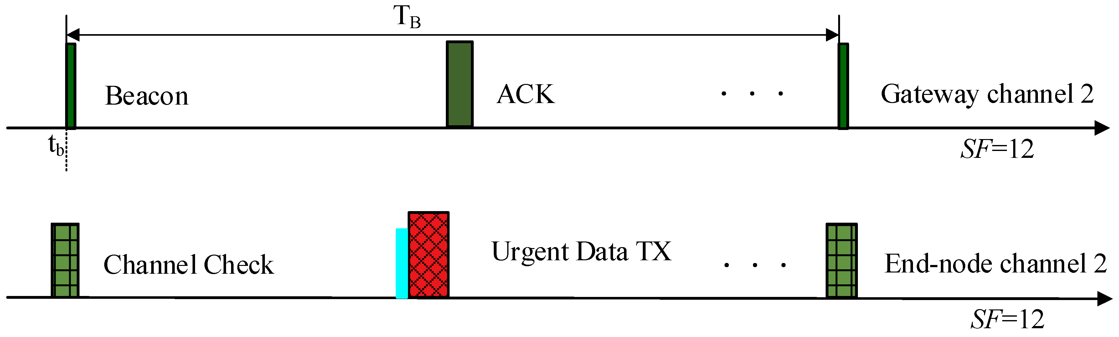
4.2.2. Schedule of Channel 2

As depicted in Figure 10, channel 2 used SF = 12, if an end-node wants to join a LoRa 2.4G network, it firstly sends a join request message (Join REQ). The gateway will respond to the join request with a join accept if the end-node is permitted to join the network.
Then, the end-node sends a synchronization request (SYN REQ), once the “TxDone” interrupt occurs, the end-node records the local timestamp t1. When the gateway receives the SYN REQ, the “RxDone” interrupt occurs. These two interrupts occur at the end-node and gateway almost simultaneously with a difference of μs range. Gateway records the local timestamp t2, then attaches t2 to the SYN ACK frame and sends it to end-node. When end-node receives the ACK frame and the “RxDone” interrupt occurs, it records the local timestamp t3 and updates its real-time clock with the new timestamp (t3 − t1 + t2). In this way both the end-node and gateway are synchronized.
There may be several concurrent transmissions on channel 2, therefore a CSMA-like mechanism was used to relieve the risk of collision. LoRa transceivers provide a special mode called channel activity detection (CAD) for channel occupancy by detecting a preamble. In channel 2, the transceivers do CAD before transmitting the packet. In case a preamble is detected, the transmitter backs off for a random period of time, then performs channel sensing again.
In DMSF–TDMA, we designed an adaptive data rate (ADR) mechanism to let end-nodes communicate at a lower SF to reduce the transmitting latency and energy consumption. The gateway estimates the wireless link status to assign the SF and time slot to the end-node. As shown in Figure 10, the end-node sent a sample request (Sample REQ) to the gateway, which contained the number of testing packets to send. Upon receiving the ACK from the gateway, the end-node did channel–sample by sending n testing packets in succession. For each testing packet received, the gateway recorded the SNR, RSSI information, and number of packets received. After receiving all the test packets, the gateway calculated R S S I ¯ , S N R ¯ (the average value of SNR and RSSI recorded), and PDR, and then selected SF ∈ {6, 7, ..., 11} according to the Expression (1).
S F = { 6 i f   S N R t h 6 < S N R ¯   a n d   R S S I t h 6 < R S S I ¯   a n d   P D R > 0.9 7 e l s e   i f   S N R t h 7 < S N R ¯   a n d   R S S I t h 7 < R S S I ¯   a n d   P D R > 0.9 n e l s e   i f   S N R t h n < S N R ¯   a n d   R S S I t h n < R S S I ¯   a n d   P D R > 0.9 11 e l s e .
S N R t h n and R S S I t h n are the thresholds of SNR and RSSI for selecting SF = n, where S N R t h n < S N R t h n 1 and R S S I t h n < R S S I t h n 1 . It means when R S S I ¯ and S N R ¯ both exceed the threshold values of a SF, the SF can be selected for the end-node. Under such condition, the lower SF value should be selected first. According to the expression (1), the threshold condition for SF = 6 was judged firstly, then condition for SF = 7, and so on. Thus, under the premise of meeting reliability, the lower SF selected for end-node means a lower time and energy cost for packet transmission. The thresholds were different in different scenarios and conditions, and could be obtained by experiments in application scenarios. For example, we could obtain the thresholds of SNR and RSSI for each SF by the aforementioned Dishui Lake experiment, as shown in Table 3.
If all time slots of the current selected SF have been allocated, the gateway continues checking the slots of (SF + 1) until an idle slot is found, and then sends the time slot number and SF to the end-node. After receiving the assigned SF and slot message, the end-node switches to Channel 1 and sets assigned SF, and then goes to sleep mode until the assigned slot time arrives.
Gateway is equipped with a GPS module to get the exact time reference, and periodically broadcasts the beacon packet in every period TB for providing the time reference and maintaining the synchronization, as shown in Figure 11. TB is an integer multiple of Tp, the time of beacon sending is at the end of the reserved zone of Tp on channel 2. To compensate for the potential clock drift of the end-node, the end-node wakes up earlier than tb by a guard time. Once “RxDone” interrupt occurs, each end-node updates the local timestamp according to the received beacon.
Figure 11 also depicts the urgent packet sending on channel 2. If the end-node senses the abnormal data or critical event occurs, it has to wait and keep sleeping until its own slot arrives. Thus, the duty cycling mechanism may induce high data latency as the wake-up intervals increases. In DMSF–TDMA, channel 1 used SF ∈ {6, 7, ..., 11}, and channel 2 used SF = 12. Since the different SFs were orthogonal, once the urgent packet occurs, the end-node can switch to channel 2, and send the packet immediately, without interfering with the transmissions of the other end-nodes on channel 1. It largely improves the real-time performance for the urgent packet.
Figure 12 is the flowchart of DMSF–TDMA for the end-node. When the end-node joins the network and finishes initialization, it switches to sleep mode to save energy and waits for a timer IRQ (interrupt request). When the IRQ arrives, it handles the program according to the IRQ type. After the IRQ processing, it switches to sleep mode again. As to the gateway, in Figure 13, it firstly initialized the channels, and then waited for the IRQ in idle mode to enhance the response speed. It handles all requests and data from the end-nodes, and maintains the network operation. For the purpose of analysis, we focused on the IRQ processes for DMSF–TDMA in flowcharts.

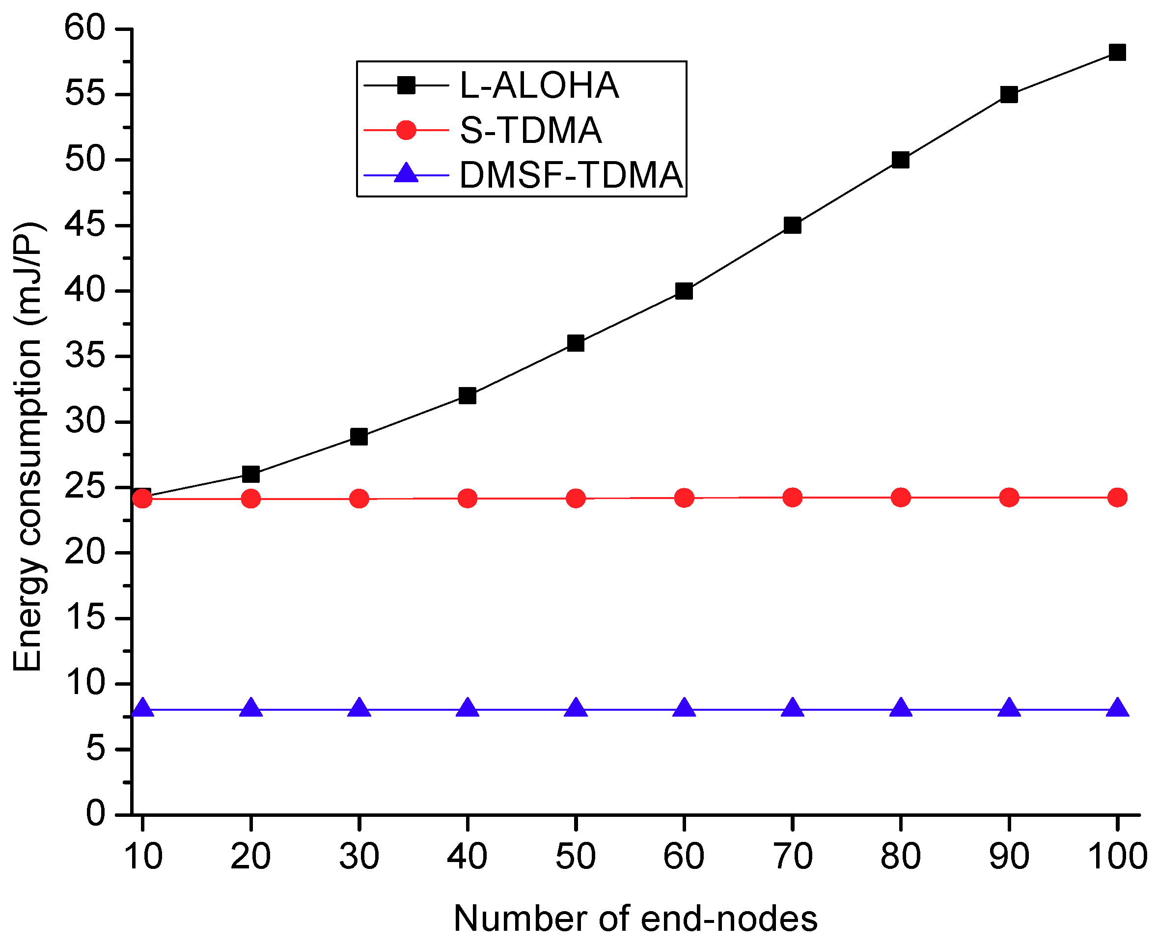
5. Performance Evaluation

To evaluate and analyze the performance of our proposed DMSF–TDMA, We built our scheme into a custom Matlab simulator based on a SX1280 transceiver. For the purposes of analysis, we assumed energy mainly consumed for the transceiver. In addition, the communication model and parameters in simulation were obtained according to the aforementioned experiments in the aquatic environment.

5.1. Simulation Model

The performance of DMSF–TDMA was compared with two different schemes: (i) Legacy LoRa using ALOHA (L-ALOHA), which is used for LoRaWAN [23,24], (ii) TDMA using single channel and single SF (S-TDMA), which is a communication mechanism used for aquatic environmental monitoring in work [13], by a set of parameters of interest in IoT.
In our simulations, we considered a scenario consisting in a circular area with a radius of 2 km, where a variable number of end-nodes was uniformly deployed and a gateway, placed in the center, was sufficient to cover all of them using SF = 11. Table 4 shows the simulation parameters for the model. The duty-cycle of each scheme did not exceed 1%, L-ALOHA and TDMA used SF = 11. All schemes had the same wake-up period, each end-node generated one packet in a wake-up period, the wake-up time offsets of end-nodes at the beginning, and the packet generation offsets of end-nodes within a period of Tp were uniformly distributed.
It was evaluated in terms of three different metrics. Firstly, energy consumption refers to the average energy cost of each end-node to successfully send a packet in a wake-up period of Tp, which can be expressed by Equations (2)–(4):
E s _ i = n ( P t x t s _ i + P r x t r _ i ) + P s t s _ i ,
T p = n ( t s _ i + t r _ i ) + t s _ i ,
E s _ a = i = 1 N E s _ i / m .
Ptx, Prx, and Ps are the power for the transmission, reception, and sleep mode. Es_i is the energy consumption of the ith end-node to successfully send a packet in a wake-up period. n is the number of retransmission, no more than 3. ts_i and tr_i are one packet transmitting time and ACK receiving time, respectively, which depend on the SF used. For example, with SF = 11 and the above setting, the transmitting time of one packet was 203 ms, and the ACK receiving time was 127 ms, which could be obtained using the SX1280 Calculator Tool. N is the total number of end-nodes, and m is the number of packets received by gateway. Thus, Es_a is the average energy cost to successfully send a packet.
Delay is defined as the time duration from packet generation to its eventual delivery to the gateway. Packet delay of the ith end-node can be expressed by t d _ i = n t s _ i + ( n 1 )   t r _ i + t g w _ i . tgw_i is the time from packet generation to node wake-up time arrival.
PDR represents the ratio of the number of packets successfully arrived at gateway to the number of packets generated by end-nodes.

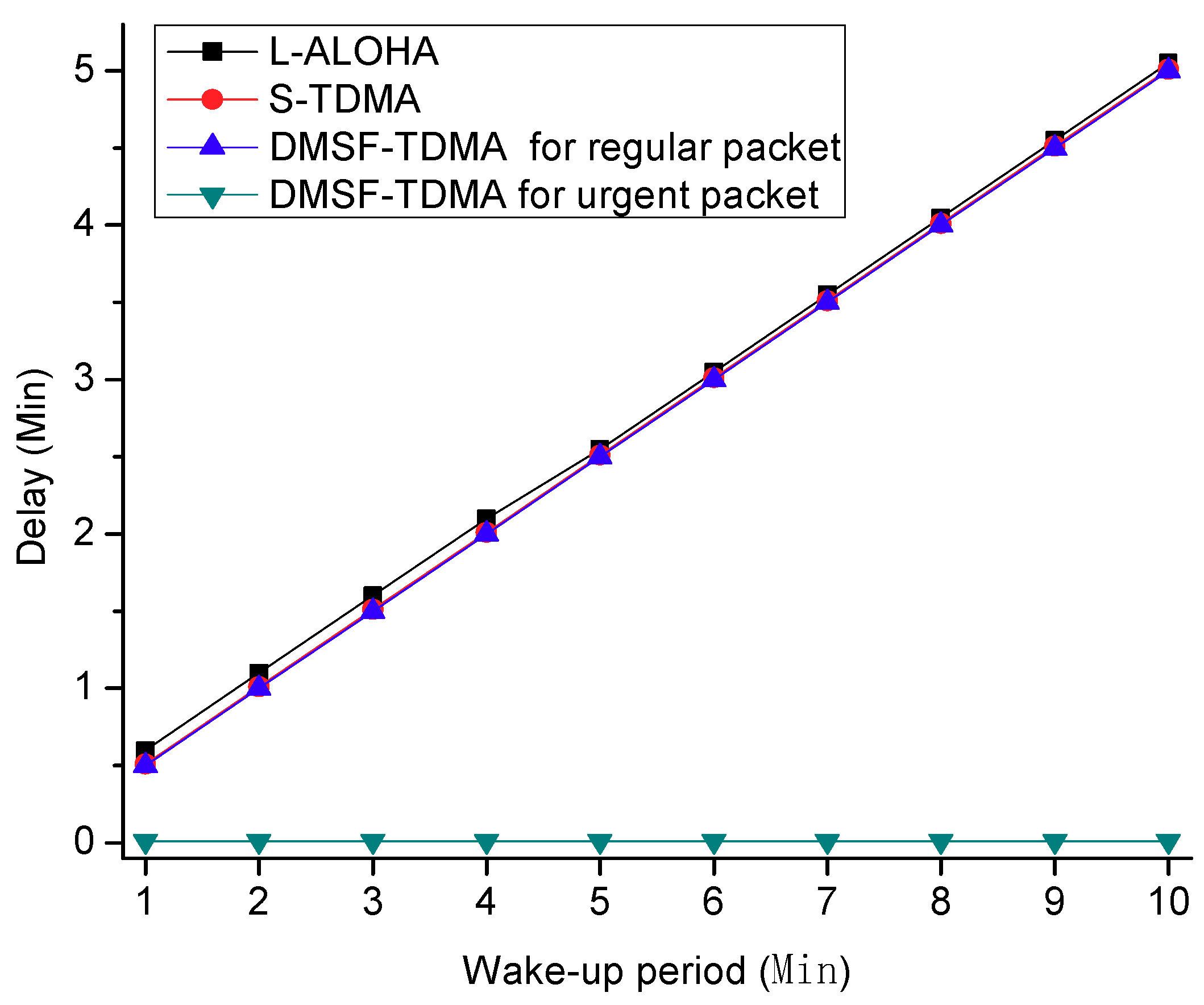
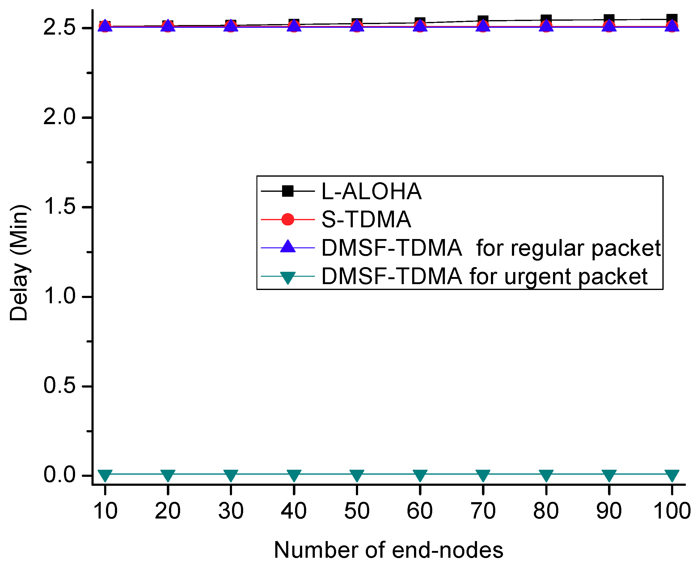
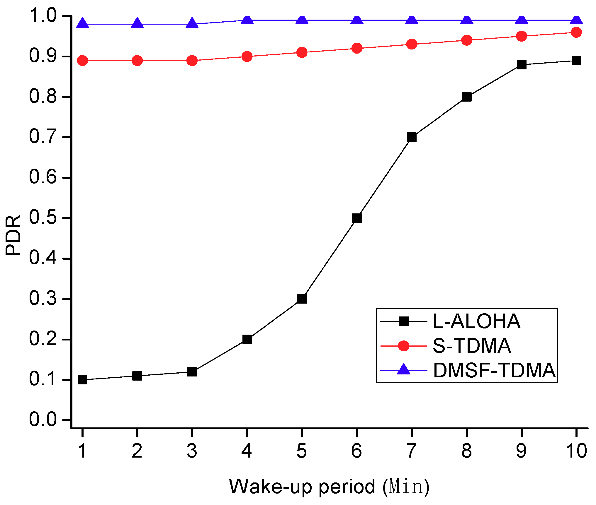
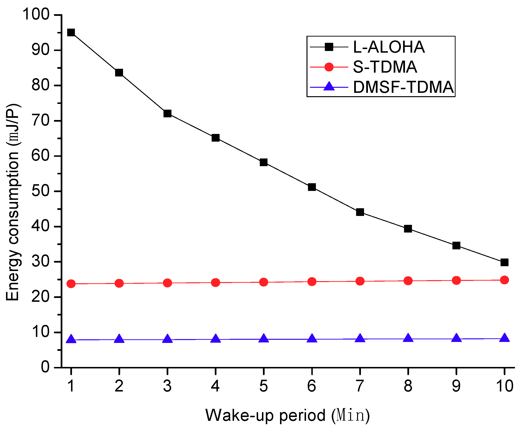
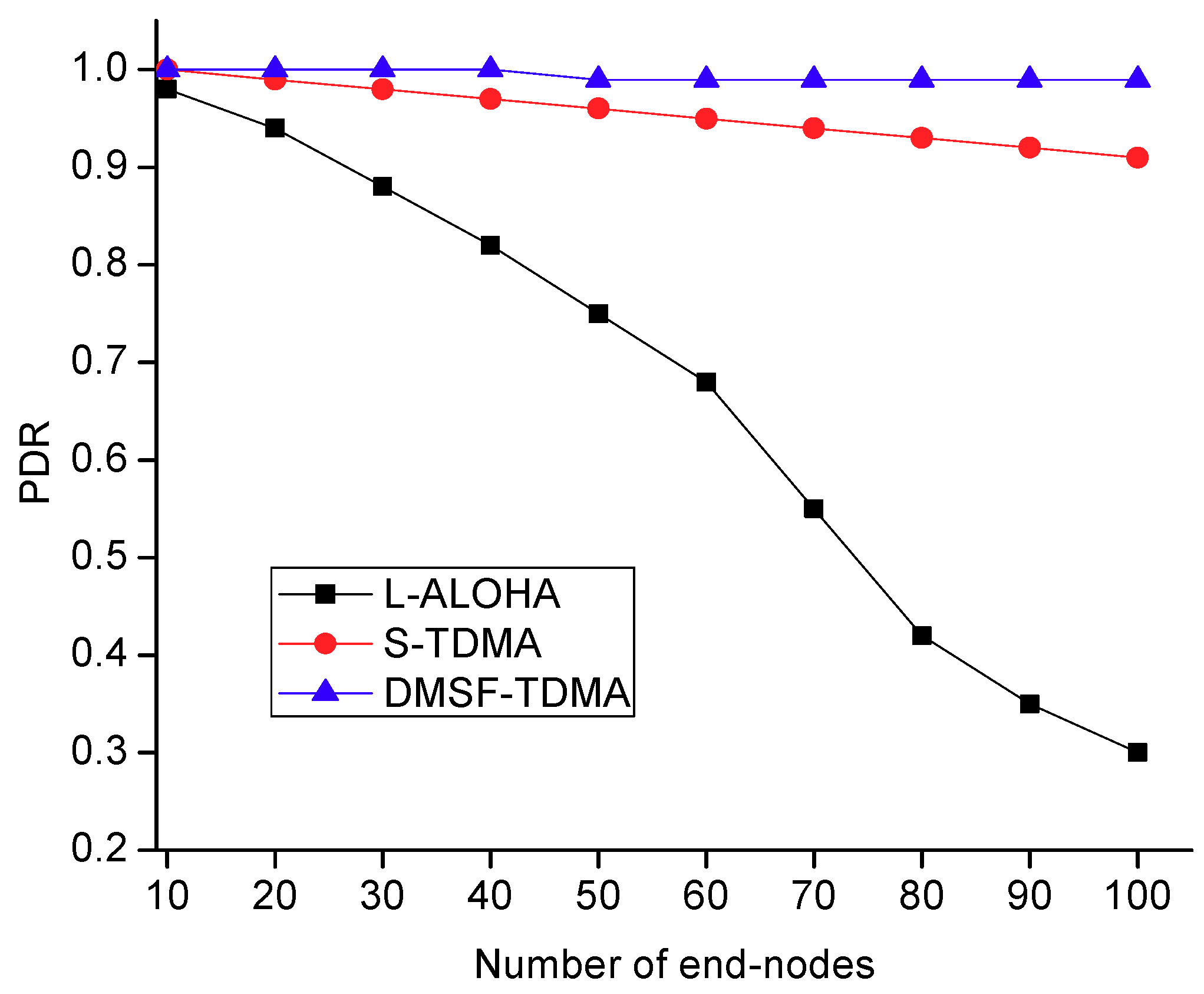
5.2. Simulation Analysis and Results

Firstly, the performance of each scheme was evaluated under different wake-up periods using 100 end-nodes.
In Figure 14, it was not surprising that DMSF–TDMA had the highest PDR, almost equal to 1, because of the independent slot for each regular packet, independent channel, and orthogonal SF for the urgent packet. With the decrease of the wake-up period, the traffic load to gateway became heavy, PDR of L-ALOHA quickly deteriorated due to the serious channel collision; when the wake-up period was less than 3 min, the PDR was down to close to 10%. S-TDMA also had a small decrease of PDR, due to using the same channel and SF for the urgent packet.
In Figure 15, all schemes except for the DMSF–TDMA for the urgent packet, incurred nearly liner growth in average delay with the increase of the wake-up period, due to the duty-cycle-based mechanism. As for L-ALOHA, packets collisions and retransmissions caused the highest latency. Multi-SF mechanism of DMSF–TDMA reduced the packet transmission latency compared with that of S-TDMA using SF = 11. In DMSF–TDMA, urgent packets were transmitted in real time using an independent channel with the orthogonal SF12, and did not wait for the arrival of the wake-up time, the packet delay was not affected by the wake-up period.
Figure 16 shows the average energy consumption of a packet transmission with different wake-up periods. The energy consumption of L-ALOHA, to successfully send a packet in a period of Tp, increased quickly with the decrease of the wake-up period. In terms of L-ALOHA, channel collision caused the retransmission of packets, which in turn further increased the traffic load and collision probability. As to DMSF–TDMA, the end-nodes closer to the gateway could be assigned to smaller SF, which means less transmission time and energy consumption for transceivers of end-nodes. Therefore, the average energy consumption of DMSF–TDMA was less than that of S-TDMA. Since TDMA mechanisms largely reduced the collision probability, both of them almost did not vary with the wake-up period.
Then, we tested the performance of each scheme under a different number of end-nodes. We fixed the wake-up period to 5 min. From the Figure 17, Figure 18 and Figure 19, we could see that as the density of end-nodes increased, traffic load to the gateway increased; the performance of L-ALOHA degraded more heavily both in PDR and energy consumption; L-ALOHA also incurred the increased delay by a few seconds.
In Figure 17, with regard to PDR, S-TDMA dropped slightly, while DMSF–TDMA could still maintain quite a high level, the analyses about PDR were the same as above.
Figure 18 depicts the average packet delay with a different number of end-nodes. Sleep latency was dominant in such low duty-cycle mode, which led to nearly a 2.5 min delay, disregarding the number of end-nodes. As for DMSF–TDMA, the delay for the urgent packet was nearly the time on the air of the packet, nearly 450 ms.
In Figure 19, with the increase of the number of end-nodes, the energy consumption difference between S-TDMA and L-ALOHA was becoming bigger and bigger. Channel collision results in the increasing energy consumption for packet transmission. If there was enough time slots for allocation, two TDMA mechanisms would not incur energy consumption rising with the density of end-nodes increasing. Average energy consumption of DMSF–TDMA was only one third of that of S-TDMA, due to the use of multiple lower SFs.
From the simulation results, the performance of DMSF–TDMA was conformed. It largely relieved the channel collision, reduced the average transmitting energy consumption, and realized the real-time sending of urgent packets. In addition, we could see that DMSF–TDMA could allocate more slots with the same wake-up period, due to assigning multiple lower SFs to end-nodes, which improved the network scalability.

6. Conclusions

In this paper, we presented a LoRa 2.4G network architecture and a DMSF–TDMA MAC scheme, using low-cost LoRa 2.4G transceiver SX1280, which considered energy efficiency while reducing channel collision and delay in the context of aquatic environmental monitoring. We implemented SX1280 point-to-point communication experiments with different scenarios over lake water, to confirm the applicability of LoRa 2.4G in an aquatic environment. The dual-channel multiple SFs scheme for a regular packet and urgent packet considered the different patterns of data sources, such as critical events, abnormal data, and periodic data gathering, further improving the PDR, real-time of urgent packets, and network scalability. The simulation results show that DMSF–TDMA achieved higher PDR while providing good performance about delay and energy consumption, compared with L-ALOHA and S-TDMA schemes.
As for DMSF–TDMA, we mainly considered the optimization scheme for uplink transmissions. In future work, we will consider the efficient schemes for downlink transmissions; and conduct the aquatic scenario experiments with more end-nodes, to further evaluate the performance of DMSF–TDMA scheme.

Author Contributions

Z.Z. proposed the idea of network architecture and DMSF–TDMA scheme. Y.W. performed the experiments and the analysis of the results. The article was written by Z.Z., S.C. and Y.W., with the assistance of S.C. on the revision of the manuscript.

Funding

This research was funded by “innovative action plan” of Science and Technology Commission of Shanghai Municipality, grant number 17050502000, and Industry-Education-Research Collaboration Project of Shanghai Lingang, grant number D-8005-18-0129. The APC was funded by 17050502000.

Acknowledgments

We thank the anonymous reviewers for their valuable comments and suggestions in improving our manuscript.

Conflicts of Interest

The authors declare no conflict of interest.

References

  1. Gubbi, J.; Buyya, R.; Marusic, S.; Palaniswami, M. Internet of Things (IoT): A vision, architectural elements, and future directions. Future Gener. Comput. Syst. 2013, 29, 1645–1660. [Google Scholar] [CrossRef] [Green Version]
  2. Bandyopadhyay, D.; Sen, J. Internet of Things: Applications and challenges in technology and standardization. Wirel. Pers. Commun. 2011, 55, 49–69. [Google Scholar] [CrossRef]
  3. Atzori, L.; Iera, A.; Morabito, G. The Internet of Things: A Survey. Comput. Netw. 2010, 54, 2787–2805. [Google Scholar] [CrossRef]
  4. Chen, Z.; Guo, Q.; Shi, Z. Design of WSN node for water pollution remote monitoring. Telecommun. Syst. 2013, 53, 155–162. [Google Scholar] [CrossRef]
  5. Bosma, R.H.; Verdegem, M.C.J. Sustainable aquaculture in ponds: Principles, practices and limits. Livest. Sci. 2011, 139, 58–68. [Google Scholar] [CrossRef]
  6. De Marziani, C.; Alcoleas, R.; Colombo, F.; Costa, N.; Pujana, F.; Colombo, A.; Aparicio, J.; Álvarez, F.J.; Jimenez, A.; Ureña, J.; et al. A low cost reconfigurable sensor network for coastal monitoring. In Proceedings of the IEEE Conference on OCEANS, Santander, Spain, 6–9 June 2011; pp. 1–6. [Google Scholar]
  7. Albaladejo, C.; Soto, F.; Torres, R.; Sánchez, P.; López, J.A. A low-cost sensor buoy system for monitoring shallow marine environments. Sensors 2012, 12, 9613–9634. [Google Scholar] [CrossRef]
  8. Liu, K.; Yang, Z.; Li, M.; Guo, Z.; Guo, Y.; Hong, F.; Yang, X.; He, Y.; Feng, Y.; Liu, Y. Oceansense: Monitoring the sea with wireless sensor networks. Mob. Comput. Commun. Rev. 2010, 14, 7–9. [Google Scholar] [CrossRef]
  9. Xu, G.; Shen, W.; Wang, X. Applications of Wireless Sensor Networks in Marine Environment Monitoring: A Survey. Sensors 2014, 14, 16932–16954. [Google Scholar] [CrossRef] [Green Version]
  10. Simbeye, D.S.; Zhao, J.; Yang, S. Design and deployment of wireless sensor networks for aquaculture monitoring and control based on virtual instruments. Comput. Electron. Agric. 2014, 102, 31–42. [Google Scholar] [CrossRef]
  11. Cano, C.; Bellalta, B.; Sfairopoulou, A.; Oliver, M. Low energy operation in WSNs: A survey of preamble sampling MAC protocols. Comput. Netw. 2011, 55, 3351–3363. [Google Scholar] [CrossRef]
  12. Anastasi, G.; Conti, M.; Francesco, M.D.; Passarella, A. Energy conservationin wireless sensor networks: A survey. Ad Hoc Netw. 2009, 7, 537–568. [Google Scholar] [CrossRef]
  13. Alippi, C.; Camplani, R.; Galperti, C.; Roveri, M. A Robust, Adaptive, Solar-Powered WSN Framework for Aquatic Environmental Monitoring. IEEE Sens. J. 2011, 11, 45–55. [Google Scholar] [CrossRef]
  14. Albaladejo Pérez, C.; Soto Valles, F.; Torres Sánchez, R.; Jiménez Buendía, M.; López-Castejón, F.; Gilabert Cervera, J. Design and Deployment of a Wireless Sensor Network for the Mar Menor Coastal Observation System. IEEE J. Ocean. Eng. 2017, 42, 1–11. [Google Scholar] [CrossRef]
  15. Faustine, A.; Mvuma, A.N.; Mongi, H.J.; Gabriel, M.C.; Tenge, A.J.; Kucel, S.B. Wireless Sensor Networks for Water Quality Monitoring and Control within Lake Victoria Basin: Prototype Development. Wirel. Sens. Netw. 2014, 6, 281–290. [Google Scholar] [CrossRef]
  16. Huang, X.; Yi, J.; Chen, S.; Zhu, X. A Wireless Sensor Network-Based Approach with Decision Support for Monitoring Lake Water Quality. Sensors 2015, 15, 29273–29296. [Google Scholar] [CrossRef] [Green Version]
  17. Hongpin, L.; Guanglin, L.; Weifeng, P.; Jie, S.; Qiuwei, B. Real-time remote monitoring system for aquaculture water quality. Int. J. Agric. Biol. Eng. 2015, 8, 136–143. [Google Scholar]
  18. Adamo, F.; Attivissimo, F.; Carducci, C.G.C.; Lanzolla, A.M.L. A Smart Sensor Network for Sea Water Quality Monitoring. IEEE Sens. J. 2015, 15, 2514–2522. [Google Scholar] [CrossRef]
  19. Chandanapalli, S.B.; Reddy, E.S.; Davuluri, D.R.L. Efficient Design and Deployment of Aqua Monitoring Systems Using WSNs and Correlation Analysis. Int. J. Comput. Commun. Control 2015, 10, 471–479. [Google Scholar] [CrossRef]
  20. Ali, A.; Shah, G.A.; Farooq, M.O.; Ghani, U. Technologies and challenges in developing Machine-to-Machine applications: A survey. J. Netw. Comput. Appl. 2017, 83, 124–139. [Google Scholar] [CrossRef]
  21. Mekki, K.; Bajic, E.; Chaxel, F.; Meyer, F. A comparative study of LPWAN technologies for large-scale IoT deployment. ICT Express 2019, 5, 1–7. [Google Scholar] [CrossRef]
  22. Augustin, A.; Yi, J.; Clausen, T.; Townsley, W.M. A Study of LoRa: Long Range & Low Power Networks for the Internet of Things. Sensors 2016, 16, 1466. [Google Scholar]
  23. Petajajarvi, J.; Mikhaylov, K.; Pettissalo, M.; Janhunen, J.; Iinatti, J. Performance of a low-power wide-area network based on lora technology: Doppler robustness, scalability, and coverage. Int. J. Distrib. Sens. Netw. 2017, 13, 1–16. [Google Scholar] [CrossRef]
  24. LoRa-Alliance. LoRaWAN Specification; Technical Report; LoRa Alliance: Beaverton, OR, USA, July 2018. [Google Scholar]
  25. Feltrin, L.; Buratti, C.; Vinciarelli, E.; De Bonis, R.; Verdone, R. LoRaWAN: Evaluation of Link- and System-Level Performance. IEEE Internet Things J. 2018, 5, 2249–2258. [Google Scholar] [CrossRef]
  26. Reynders, B.; Wang, Q.; Tuset-Peiro, P.; Vilajosana, X.; Pollin, S. Improving reliability and scalability of lorawans through lightweight scheduling. IEEE Internet Things J. 2018, 5, 1830–1842. [Google Scholar] [CrossRef]
  27. Li, L.; Ren, J.; Zhu, Q. On the application of LoRa LPWAN technology in Sailing Monitoring System. In Proceedings of the 13th Annual Conference on Wireless On-demand Network Systems and Services (WONS), Jackson, WY, USA, 21–24 February 2017; pp. 77–80. [Google Scholar]
  28. Petajajarvi, J.; Mikhaylov, K.; Roivainen, A.; Hanninen, T.; Pettissalo, M. On the coverage of LPWANs: Range evaluation and channel attenuation model for lora technology. In Proceedings of the 14th International Conference on ITS Telecommunications (ITST), Copenhagen, Denmark, 2–4 December 2015; pp. 55–59. [Google Scholar]
  29. Sanchez-Iborra, R.G.; Liaño, I.; Simoes, C.; Couñago, E.; Skarmeta, A. Tracking and Monitoring System Based on LoRa Technology for Lightweight Boats. Electronics 2019, 8, 15. [Google Scholar] [CrossRef]
  30. Jovalekic, N.; Drndarevic, V.; Pietrosemoli, E.; Zennaro, I. Experimental Study of LoRa Transmission over Seawater. Sensors 2018, 18, 2853. [Google Scholar] [CrossRef]
  31. Georgiou, O.; Raza, U. Low power wide area network analysis: Can LoRa scale? IEEE Wirel. Commun. Lett. 2017, 6, 162–165. [Google Scholar] [CrossRef]
  32. Mikhaylov, K.; Petäjäjärvi, J.; Haenninen, T. Analysis of capacity and scalability of the LoRa low power wide area network technology. In Proceedings of the European Wireless 2016, 22th European Wireless Conference, Oulu, Finland, 18–20 May 2016; pp. 119–125. [Google Scholar]
  33. Piyare, R.; Murphy, A.; Magno, M.; Benini, L. On-demand lora: Asynchronous tdma for energy efficient and low latency communication in iot. Sensors 2018, 18, 3718. [Google Scholar] [CrossRef]
  34. Pham, C. Enabling and deploying long-range IoT image sensors with LoRa technology. In Proceedings of the 2018 IEEE Middle East and North Africa Communications Conference (MENACOMM), Jounieh, Lebanon, 18–20 April 2018; pp. 1–6. [Google Scholar]
  35. Dinh, N.T.; Kim, Y. Information-centric dissemination protocol for safety information in vehicular ad-hoc networks. Wirel. Netw. 2017, 23, 1359–1371. [Google Scholar] [CrossRef]
  36. Dinh, T.; Kim, Y.; Gu, T.; Vasilakos, A.V. L-mac: A wake-up time self-learning mac protocol for wireless sensor networks. Comput. Netw. 2016, 105, 33–46. [Google Scholar] [CrossRef]
  37. SX1280 Transceivers. July 2019. Available online: https://www.semtech.com/uploads/documents/ DS_SX1280-1_V2.2.pdf (accessed on 19 July 2019).
Figure 1. Map of Dishui Lake experiments and the sending and receiving nodes’ locations.
Electronics 08 00909 g001
Figure 2. The sending nodes with different height locations above water level at Site B.
Electronics 08 00909 g002
Figure 3. Performance testing at Site B.
Electronics 08 00909 g003
Figure 4. Performance testing at Site C.
Electronics 08 00909 g004
Figure 5. Performance testing at Site D.
Electronics 08 00909 g005
Figure 6. The measurements of the relationship between RSSI and distance.
Electronics 08 00909 g006
Figure 7. Network architecture.
Electronics 08 00909 g007
Figure 8. Protocol architecture.
Electronics 08 00909 g008
Figure 9. The channel 1 of dual-channel multiple spreading factors–time division multiple access (DMSF–TDMA).
Electronics 08 00909 g009
Figure 10. End-nodes join the network on channel 2.
Electronics 08 00909 g010
Figure 11. Beacon and urgent packet sending on channel 2.
Electronics 08 00909 g011
Figure 12. The flowchart of DMSF–TDMA for the end-node.
Electronics 08 00909 g012
Figure 13. The flowchart of DMSF–TDMA for the gateway.
Electronics 08 00909 g013
Figure 14. Average packet delivery ratio (PDR) with different wake-up periods.
Electronics 08 00909 g014
Figure 15. Average delay with different wake-up periods.
Electronics 08 00909 g015
Figure 16. Average energy consumption with different wake-up periods.
Electronics 08 00909 g016
Figure 17. Average PDR with a different number of end-nodes.
Electronics 08 00909 g017
Figure 18. Average delay with a different number of end-nodes.
Electronics 08 00909 g018
Figure 19. Average energy consumption with a different number of end-nodes.
Electronics 08 00909 g019
Table 1. SX1280 raw data rates with different spreading factors (SFs) and bandwidth.
Bandwidth (kHz)Raw Data Rates (kb/s)
SF5SF6SF7SF8SF9SF10SF11SF12
20331.7219.0311.16.343.571.981.090.595
40663.4438.0622.212.697.143.962.181.19
812126.8876.1344.4125.3814.277.934.362.38
1625253.91152.3488.8750.7828.5615.878.734.76
Table 2. Typical transceiver parameters comparison.
TransceiverSX1278SX1280CC2520
ModulationLoRaLoRaIEEE 802.15.4
Band470 MHz2.4 GHz2.4 GHz
Data rate (Max)37.5 kb/s202 kb/s250 kb/s
Receiver sensitivity−148 dBm−132 dBm−98 dBm
Tx current29 mA @ + 13 dBm24 mA @ + 12.5 dBmTX 33.6 mA @ + 5 dBm
RX current9.9 mA8.2 mA18.5 mA
Table 3. The thresholds of the signal-to-noise ratio (SNR) and RSSI for each SF.
SFSNRRSSI
60−85
70−90
8−5−95
9−10−108
10−15−115
Table 4. Simulation parameters.
ParameterValue
LoRa SettingBW = 406 kHz, CR = 4/5, SF ∈ (6, 12), Preamble length = 8 symbol
Rx current6.7 mA
Tx current24 mA@ + 12.5 dBm
Sleep current0.4 μA
Payload16 Bytes
Beacon period20 min

