Enhanced Switch Image-Based Visual Servoing Dealing with FeaturesLoss

Abstract

In this paper, an enhanced switch image-based visual servoing controller for a six-degree-of-freedom (DOF) robot with a monocular eye-in-hand camera configuration is presented. The switch control algorithm separates the rotating and translational camera motions and divides the image-based visual servoing (IBVS) control into three distinct stages with different gains. In the proposed method, an image feature reconstruction algorithm based on the Kalman filter is proposed to handle the situation where the image features go outside the camera’s field of view (FOV). The combination of the switch controller and the feature reconstruction algorithm improves the system response speed and tracking performance of IBVS, while ensuring the success of servoing in the case of the feature loss. Extensive simulation and experimental tests are carried out on a 6-DOF robot to verify the effectiveness of the proposed method.

1. Introduction

Visual servoing has been employed to increase the deftness and intelligence of industrial robots, especially in unstructured environments [1,2,3,4]. Based on how the image data are used to control the robot, visual servoing is classified into two categories: position-based visual servoing (PBVS) and image-based visual servoing (IBVS). A comprehensive analysis of the advantages and drawbacks of the aforementioned methods can be found in [5]. This paper focuses on addressing some issues in IBVS.

Many studies have been conducted to overcome the weaknesses of IBVS and improve its efficiency [6,7,8,9]. However, the performance of most reported IBVS is not sufficiently high to meet the requirements of industrial applications [10]. An efficient IBVS feasible for practical robotic operations requires a fast response with strong robustness to feature loss. One obvious way to increase the speed of IBVS is to increase the gain values in the control law. However, there is a limitation on the application of this strategy because the high gain in the IBVS controller tends to create shakiness and instability in the robotic system [11]. Moreover, the stability of the traditional IBVS system is proven only in an area around the desired position [5,12]. Furthermore, when the initial feature configuration is distant from the desired one, the converging time is long, and possible image singularities may lead to IBVS failure. To address this issue, a switching scheme is proposed to switch the control signal between low-level visual servo controllers, i.e., homography-based controller [13] and affine-approximation controller [14]. In our previous work [15,16], the idea of switch control in IBVS was proposed to switch the controller between end-effector’s rotating and translational movements. Although it has been demonstrated that the switch control can improve the speed and tracking performance of IBVS and avoid some of its inherent drawbacks, feature loss caused by the camera’s limited FOV still prevents the method from being fully efficient and being applicable to real industrial robots.

The visual features contain much information such as the robots’ pose information, the tasks’ states, the influence of the environment, the disturbance to the robots, etc. The features are directly related to the motion screw of the end-effector of the robot. The completeness of the feature set during visual servoing is key to fulfilling the task successfully. Many features have been used in visual servoing such as feature points, image moments, lines, etc. The feature points are known for the ease of image processing and extraction. It is shown that at least three image points are needed for controlling a 6-DOF robot [17]. Hence, four image points are usually used for visual servoing. However, the feature points tend to leave the FOV during the process of visual servoing. A strategy is needed to handle the situation where the features are lost.

There are two main approaches to handle feature loss and/or occlusion caused by the limited FOV of the camera [18]. In the first approach, the controller is designed to avoid occlusion or feature loss, while in the second one, the controller is designed to handle the feature loss.

In the first approach, several techniques have been developed to avoid the feature loss or occlusion. In [19], occlusion avoidance was considered as the second task besides the primary visual servoing task. In [20], a reactive unified convex optimization-based controller was designed to avoid occlusion during teleoperation of a dual-arm robot. Some studies have been carried out in visual trajectory planning considering feature loss avoidance [21,22,23]. Model predictive control methods have been adopted in visual servoing to prevent feature loss due to its ability to deal with constraints [24,25,26,27,28]. In [29], predictive control was employed to handle visibility, workspace, and actuator constraints. Despite the success of the studies on preventing feature loss, they suffered from the limited maneuvering workspace of the robot, due to the conservative design required to satisfy many constraints.

In the second approach, the controller tries to handle the feature loss instead of avoiding it. When the loss or occlusion of features occurs, if the remaining visible features are sufficient to generate the non-singular inverse of the image Jacobian matrix, the visual servoing task can still be carried out successfully. In this situation, the rank of the relative Jacobian matrix must be the same as the degrees of freedom [30]. However, this method is no longer effective when the number of remaining visible features become too small to guarantee the full-rankness of the image Jacobian matrix. As studied in [31], another solution is to foresee the position of the lost features and to continue the control process using the predicted features until they become visible again. This method allows partial or complete loss or occlusion of the features. In the second approach [30,31], the classical IBVS control is employed as the control method, which does not usually provide a fast response.

In this paper, an enhanced switch image-based visual servoing (ESIBVS) method is presented in which a Kalman filter-based feature prediction algorithm is proposed and is combined with our previous work [15,16] to make the switch IBVS control robust in reaction to feature loss. The feature prediction algorithm can predict the lost feature points based on the previously-estimated points. The switch control with the improved tracking performance along with the robustness to feature loss makes it more feasible for industrial robotic applications. To validate the proposed controller, extensive simulations and experiments have been conducted on a 6-DOF Denso robot with a monocular eye-in-hand vision system.

The structure of the paper is given as follows. Section 2 gives a description of the problem. In Section 3, the feature reconstruction algorithm is presented. In Section 4, the controller design algorithm is developed. In Section 5, the simulation results are given. Experimental results are presented in Section 6, and finally, the concluding remarks are given in Section 7.

2. Problem Statement

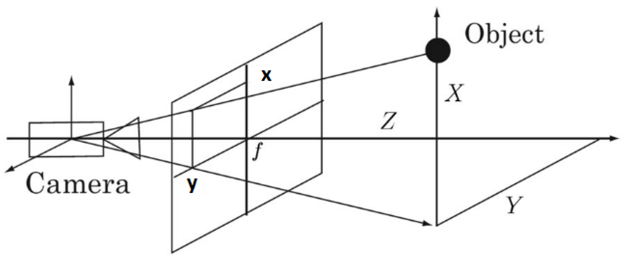
In IBVS, the object with $(X,Y,Z)$ coordinates with respect to camera has the projected image coordinates $(x,y)$ in the camera image (Figure 1). The feature’s positions and the desired ones for the $n^{\mathrm{th}}$ feature in the image plane can be denoted by:

$$s_n={\left[x_n{y}_n\right]}^T,s_{dn}={\left[x_{dn}{y}_{dn}\right]}^T$$

(1)

Thus, the vector of s and $s_d$ is defined as:

$$s=\left[\begin{array}{c}{s}_1\\ ⋮\\ s_n\end{array}\right]=\left[\begin{array}{c}{x}_1\\ y_1\\ ⋮\\ x_n\\ y_n\end{array}\right],s_d=\left[\begin{array}{c}{s}_{d1}\\ ⋮\\ s_{dn}\end{array}\right]=\left[\begin{array}{c}{x}_{d1}\\ y_{d1}\\ ⋮\\ x_{dn}\\ y_{dn}\end{array}\right].$$

(2)

The goal of the IBVS task is to generate camera velocity commands such that the actual features and the desired ones are matched in the image plane. The velocity of the camera is defined as $V_c\left(t\right)$. The camera and image feature velocities are related by:

$$\dot{s}=J_{img}{V}_c,$$

(3)

where,

$$J_{img}=\left[\begin{array}{c}{J}_{img}(s_1,Z_1)\\ ⋮\\ J_{img}(s_n,Z_n)\end{array}\right],$$

(4)

which is called the image Jacobian matrix and $Z_1,\cdots ,Z_n$ are the depths of the features $s_1,\dots ,s_n$. In this study, the system configuration is set as eye-in-hand, and the number of features is $n=4$. Furthermore, it is assumed that all the features share the same depth Z. Considering these assumptions, the image Jacobian matrix for the $n^{\mathrm{th}}$ feature is given in [17]:

$$\begin{array}{c}\hfill J_{img}\left(s_n\right)=\left[\begin{array}{cccccc}\frac{f}{Z}& 0& -\frac{x_n}{Z}& -\frac{x_n{y}_n}{f}& \frac{f^2+x_n^2}{f}& -y_n\\ 0& \frac{f}{Z}& -\frac{y_n}{Z}& \frac{-f^2-y_n^2}{f}& \frac{x_n{y}_n}{f}& x_n\end{array}\right],\end{array}$$

(5)

where f is the focal length of the camera.

The velocity of the camera can be calculated by manipulating (3):

$$V_c=\stackrel{+}{J_{img}}\dot{s},$$

(6)

where $\stackrel{+}{J_{img}}$ is the pseudo-inverse of the image Jacobian matrix. The error signal is defined as $e=s-s_d$. If we let $\dot{e}=-K_{a}e$, the traditional IBVS control law may be designed as:

$$V_c=-K_a\stackrel{+}{J_{img}}e,$$

(7)

where $K_a$ is the proportional gain.

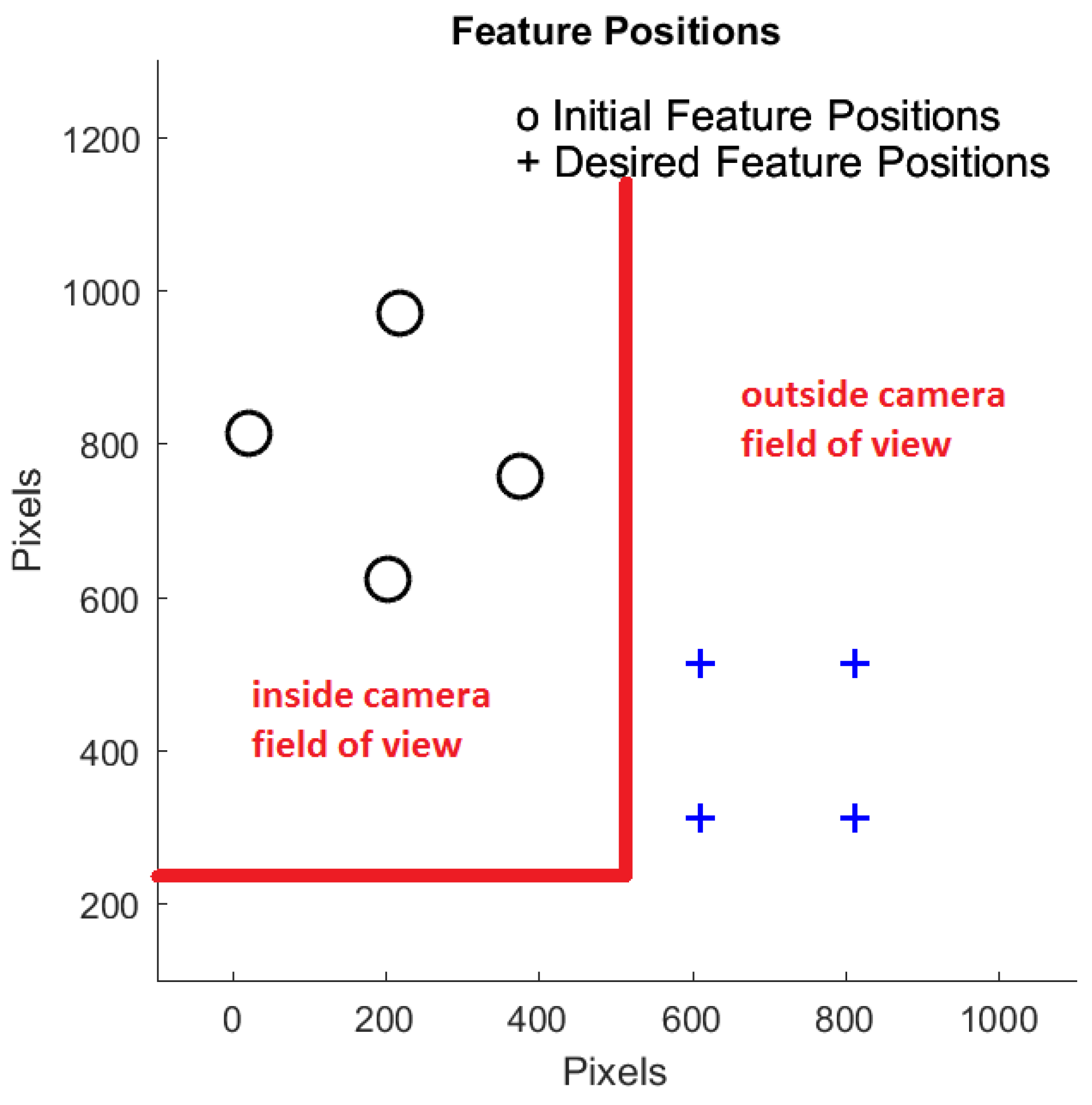
While guiding the robot end-effector to make the desired image features match the actual ones, some unexpected situations may occur in IBVS. The first case is feature loss: i.e., some or all of the image features may go beyond the camera’s FOV (Figure 2). The second case is feature occlusion: i.e., some or all of the image features temporarily become invisible to the camera due to obstacles. The goal of this paper is to improve the performance of IBVS in terms of response time and tracking performance, while dealing with the feature loss situation. To reach this goal, the performance of the switch method in our previous work [15,16] is enhanced when it is combined with the proposed feature reconstruction algorithm.

3. Feature Reconstruction Algorithm

The velocity of the camera $V_c\in {\mathbb{R}}^{(6\times 1)}$ can be divided into the translational velocity $V\in {\mathbb{R}}^{(3\times 1)}$ and rotating velocity $\omega \in {\mathbb{R}}^{(3\times 1)}$. Therefore, it can be expressed as:

$$V_C=\left[\begin{array}{c}V\\ \omega \end{array}\right]=\left[\begin{array}{c}{V}_x\\ V_y\\ V_z\\ {\omega }_x\\ {\omega }_y\\ {\omega }_z\end{array}\right],$$

(8)

Furthermore, for the $n^{\mathrm{th}}$ feature $(n=1,2,\dots ,4)$, the image Jacobian matrix in (5) can be divided into the translational part $J_t\left(s_n\right)$ and the rotating part $J_r\left(s_n\right)$:

$$J_{img}\left(s_n\right)=\left[\begin{array}{c}{J}_t\left(s_n\right)J_r\left(s_n\right)\end{array}\right],$$

(9)

where,

$$J_t\left(s_n\right)=\left[\begin{array}{ccc}\frac{f}{Z}& 0& -\frac{x_n}{Z}\\ 0& \frac{f}{Z}& -\frac{y_n}{Z}\end{array}\right]$$

(10)

and:

$$J_r\left(s_n\right)=\left[\begin{array}{ccc}-\frac{x_n{y}_n}{f}& \frac{f^2+x_n^2}{f}& -y_n\\ \frac{-f^2-y_n^2}{f}& \frac{x_n{y}_n}{f}& x_n\end{array}\right],$$

(11)

where $x_n$ and $y_n$ are the feature coordinates in the image space.

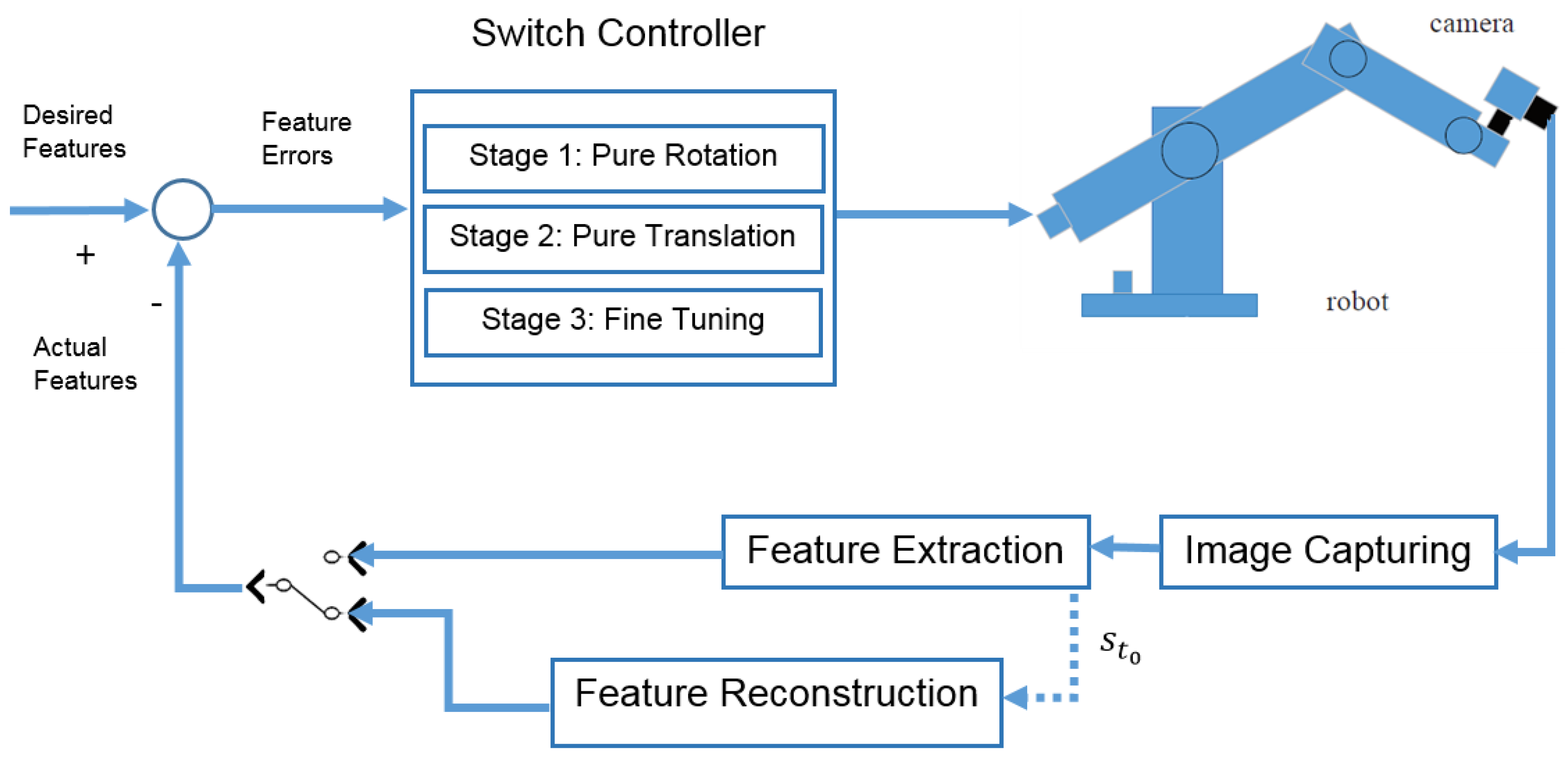
In the design of the switch controller, the movement of the camera during the control task is divided into three different stages [15,16]. In the first stage, the camera has only pure rotation. In the second stage, the camera has only translational movement. Finally, in the third stage, both camera rotation and translation are used to carry out the fine-tuning.

Considering (3), (8), (10) and (11), the feature velocity in the image plane can be expressed as:

In the pure translational stage (first stage):

$$\left\{\begin{array}{c}{\dot{x}}_n=\frac{f}{Z}{V}_x-\frac{x_n}{Z}{V}_z\\ {\dot{y}}_n=\frac{f}{Z}{V}_y-\frac{y_n}{Z}{V}_z.\end{array}\right.$$

(12)

In the pure rotating stage (second stage):

$$\left\{\begin{array}{c}{\dot{x}}_n=-\frac{x_n{y}_n}{f}{\omega }_x+\frac{f^2+x_n^2}{f}{\omega }_y-y_n{\omega }_z\\ {\dot{y}}_n=-\frac{f^2+y_n^2}{f}{\omega }_x+\frac{x_n{y}_n}{f}{\omega }_y+x_n{\omega }_z\end{array}\right.,$$

(13)

and in the fine-tuning stage (third stage):

$$\left\{\begin{array}{c}{\dot{x}}_n=\frac{f}{Z}{V}_x-\frac{x_n}{Z}{V}_z-\frac{x_n{y}_n\left(t_0\right)}{f}{\omega }_x+\frac{f^2+x_n^2}{f}{\omega }_y-y_n{\omega }_z\\ {\dot{y}}_n=\frac{f}{Z}{V}_y-\frac{y_n}{Z}{V}_z-\frac{f^2+y_n^2}{f}{\omega }_x+\frac{x_n{y}_n}{f}{\omega }_y+x_n{\omega }_z\end{array}\right..$$

(14)

To remove the noise in the image processing and feature extraction, a feature state estimator is designed based on the Kalman filter algorithm.

In the formulations below, k denotes the current time instant and $k+1$ the next time instant, while $T_s$ represents the sampling time. The estimated states are denoted by $\widehat{}$ notation. Considering four features, the feature state at the current instant ($k^{\mathrm{th}}$ sample) is defined as:

$$\begin{array}{c}\hfill X\left(k\right)={[x_1\left(k\right),y_1\left(k\right),\dots x_4\left(k\right),y_4\left(k\right),{\dot{x}}_1\left(k\right),{\dot{y}}_1\left(k\right),\dots ,{\dot{x}}_4\left(k\right),{\dot{y}}_4\left(k\right)]}^T,\end{array}$$

(15)

or with consideration of (2):

$$\begin{array}{c}\hfill X\left(k\right)=[s\left(k\right),\dot{s}\left(k\right)],\end{array}$$

(16)

where the elements of the vector can be obtained from (12), (13), or (14). Furthermore, the measurement vector represents the vector of the image feature points’ coordinates extracted from the images of the camera:

$$\begin{array}{c}\hfill M\left(k\right)={[x_{m1}\left(k\right),y_{m1}\left(k\right),\dots x_{m4}\left(k\right),y_{m4}\left(k\right),{\dot{x}}_{m1}\left(k\right),{\dot{y}}_{m1}\left(k\right),\dots ,{\dot{x}}_{m4}\left(k\right),{\dot{y}}_{m4}\left(k\right)]}^T\end{array}$$

(17)

First, the prediction equations are:

$$\begin{array}{c}\hfill \widehat{X}\left(k\right|k-1)=A\widehat{X}(k-1|k-1)\\ \hfill P\left(k\right|k-1)=AP(k-1|k-1)A^T+Q(k-1),\end{array}$$

(18)

where A is a $16\times 16$ matrix whose diagonal elements equal one, $A_{i,i+8}(i=1,2\dots ,8)$ are equal to sampling time $T_s$, and the rest of the elements are zero, $P\left(k\right|k-1)$ represents the current prediction of the error covariance matrix, which gives a measure of the state estimate accuracy, while $P(k-1|k-1)$ is the previous error covariance matrix, and $Q(k-1)$ represents the process noise covariance computed using the information of the time instant $(k-1)$.

Second, the Kalman filter gain $D\left(K\right)$ is:

$$D\left(k\right)=P\left(k\right|k-1)(P\left(k\right|k-1)+R{(k-1)}^{-1},$$

(19)

where $R(k-1)$ is the previous measurement covariance matrix.

Third, the estimation update is given as follows:

$$\begin{array}{c}\hfill \widehat{X}\left(k\right|k)=\widehat{X}\left(k\right|k-1)+D\left(k\right)(M\left(k\right)-\widehat{X}\left(k\right|k-1)\\ \hfill P\left(k\right|k)=P(K|k-1)-D\left(k\right)P\left(k\right|k-1),\end{array}$$

(20)

When the features are out of the FOV of the camera (i.e. $x_{mj}\left(k\right)=0$, $y_{mj}\left(k\right)=0$, $j=1,2,\dots ,4$), the feature reconstruction algorithm is proposed to provide the updated estimation vector under this circumstance. Since the features are out of FOV, the measurement vector will have some elements with zero values. This measurement vector will not lead to a satisfactory performance of switch IBVS. In order to improve the performance, instead of having zero values of the elements of $M\left(k\right)$ in (17), it is reasonable to assume that the $n^{\mathrm{th}}$ feature that goes outside of FOV keeps its velocity at the moment ($t_0$) of leaving (${\dot{s}}_n\left(t_0\right)$) during the period of feature loss. Hence, its position (i.e., point coordinates $s_n\left(t_0\right)=[x_{mn}\left(t_0\right),y_{mn}\left(t_0\right)$]) can be generated by integrating the velocity over the time. This means that the elements of $M\left(k\right)$ can be represented by this formulation:

$$M\left(k\right)=[(K_{ad}\sum _{l=0}^b{\dot{s}}_n\left(t_0\right)T_s+s_n\left(t_0\right)),{\dot{s}}_n\left(t_0\right)],$$

(21)

where $(l=0,1,2,\dots ,b)$ represents the number of time samples during the feature loss period, $T_s$ is the sampling period, and $k_{ad}$ is an adjusting coefficient. Once the feature is visible to the camera again, the actual value of $M\left(k\right)$ provided by the camera is used to replace the state estimation (21).

4. Controller Design

The IBVS controller was designed using the switch scheme. This method can set distinct gain values for the stages of the control law to achieve a fast response system while preserving the system stability.

In order to design the switch controller, the movement of the camera during the control task was divided into three different stages [15,16]. A criterion was needed for the switch condition between stages. In [15], the norm of feature errors was defined as the switching criterion. In this paper, a more intuitive and effective criterion is used [16]. As is shown in Figure 3, the switch angle criterion $\alpha$ is introduced as the angle between actual features and the desired ones. As soon as the angle $\alpha$ meets the predefined value, the controller law switches to the next stage.

Based on this criterion, the switching control law is presented as follows:

$$\left\{\begin{array}{c}{V}_{cs1}=-K_1{J}_r^{+}e\left(s\right),\left|\alpha \right|\ge {\alpha }_0\\ V_{cs2}=-K_2{J}_t^{+}e\left(s\right),{\alpha }_1\le \left|\alpha \right|<{\alpha }_0\\ V_{cs3}=-K_3{J}_{img}^{+}e\left(s\right),otherwise\end{array}\right.,$$

(22)

where $V_{csi}$ ($i=1,2,3$) is the velocity of the camera in the $i^{\mathrm{th}}$ stage, $K_i$ is the symmetric positive definite gain matrix at each stage, and ${\alpha }_0$ and ${\alpha }_1$ are two predefined thresholds for the control law to switch to the next stage. The block diagram of the proposed algorithm is shown in Figure 4. Furthermore, the flowchart of the whole process of feature reconstruction and control is illustrated in Figure 5.

It was expected that in comparison with switch IBVS, the proposed method would ensure the smooth transition of the visual servoing task in the case of the feature loss and provide a better convergence performance.

5. Simulation Results

To evaluate the performance of the proposed method, simulation tests were carried out by using MATLAB/SIMULINK software with the Vision and Robotic Toolbox. A 6-DOF DENSO robot with a camera installed in eye-in-hand configuration was simulated. The coordinates of the initial and desired features in the image space are given in

Table 1. Test 1: simulation. Initial (I) and desired (D) feature point positions in pixels.

		Point 1		Point 2		Point 3		Point 4
		(x, y)		(x, y)		(x, y)		(x, y)
Test 1	I	376	757	202	621	20	814	218	969
	D	612	312	612	512	812	512	812	312

. The camera parameters are as shown in

Table 2. Camera parameters.

Parameter	Value
Focal length (m) (f)	0.004
x axis scaling factor (pixel/m) ($\beta$)	110,000
y axis scaling factor (pixel/m) ($\beta$)	110,000
Principal point of x axis (pixel) ($c_u$)	120
Principal point of y axis (pixel) ($c_v$)	187

.

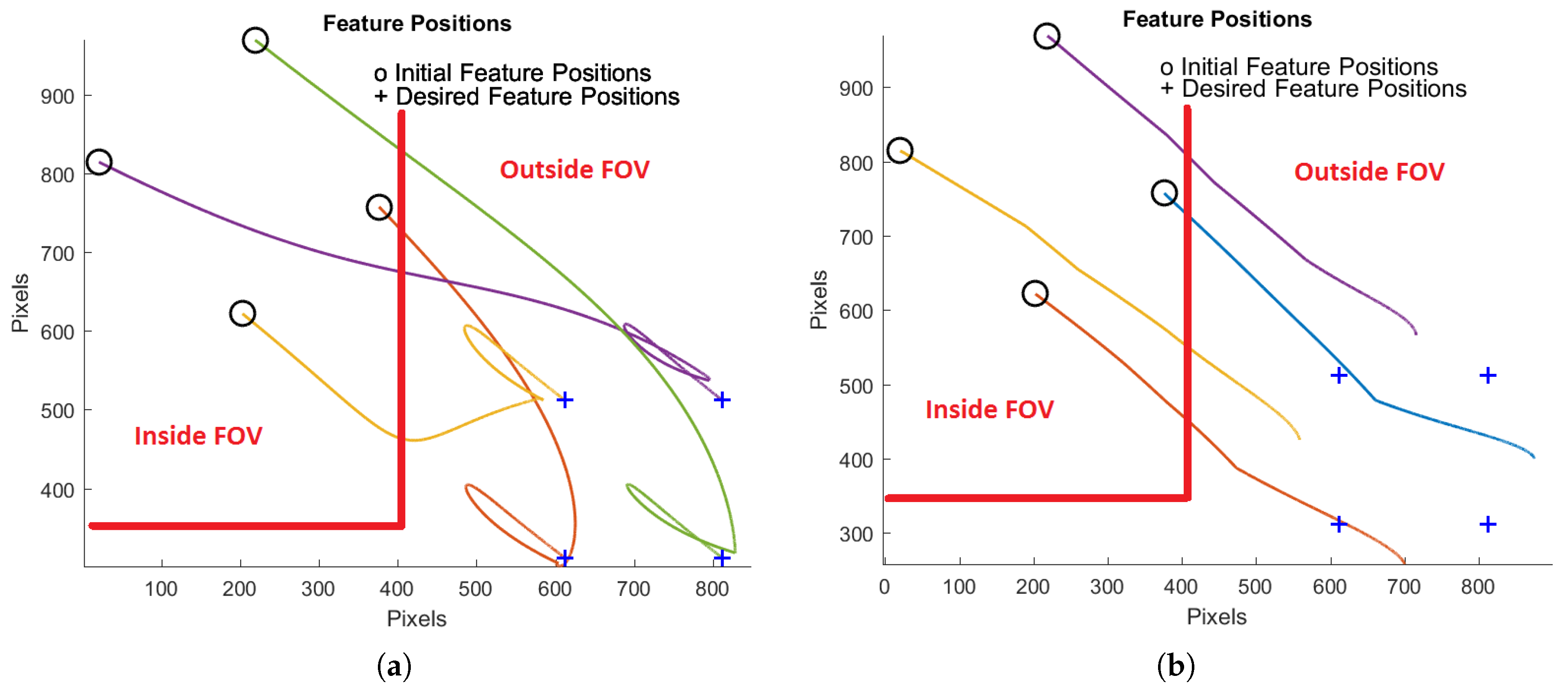
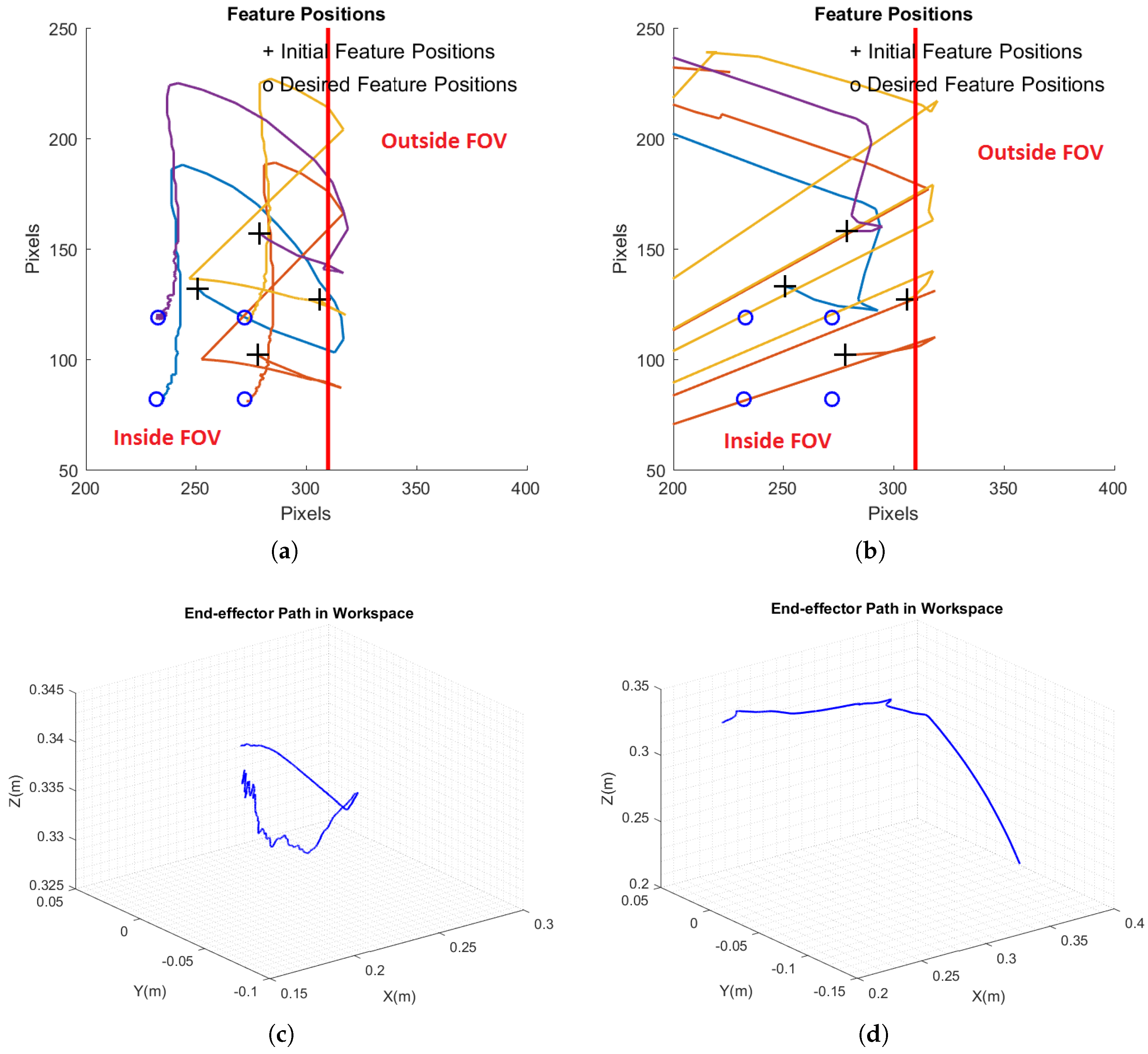
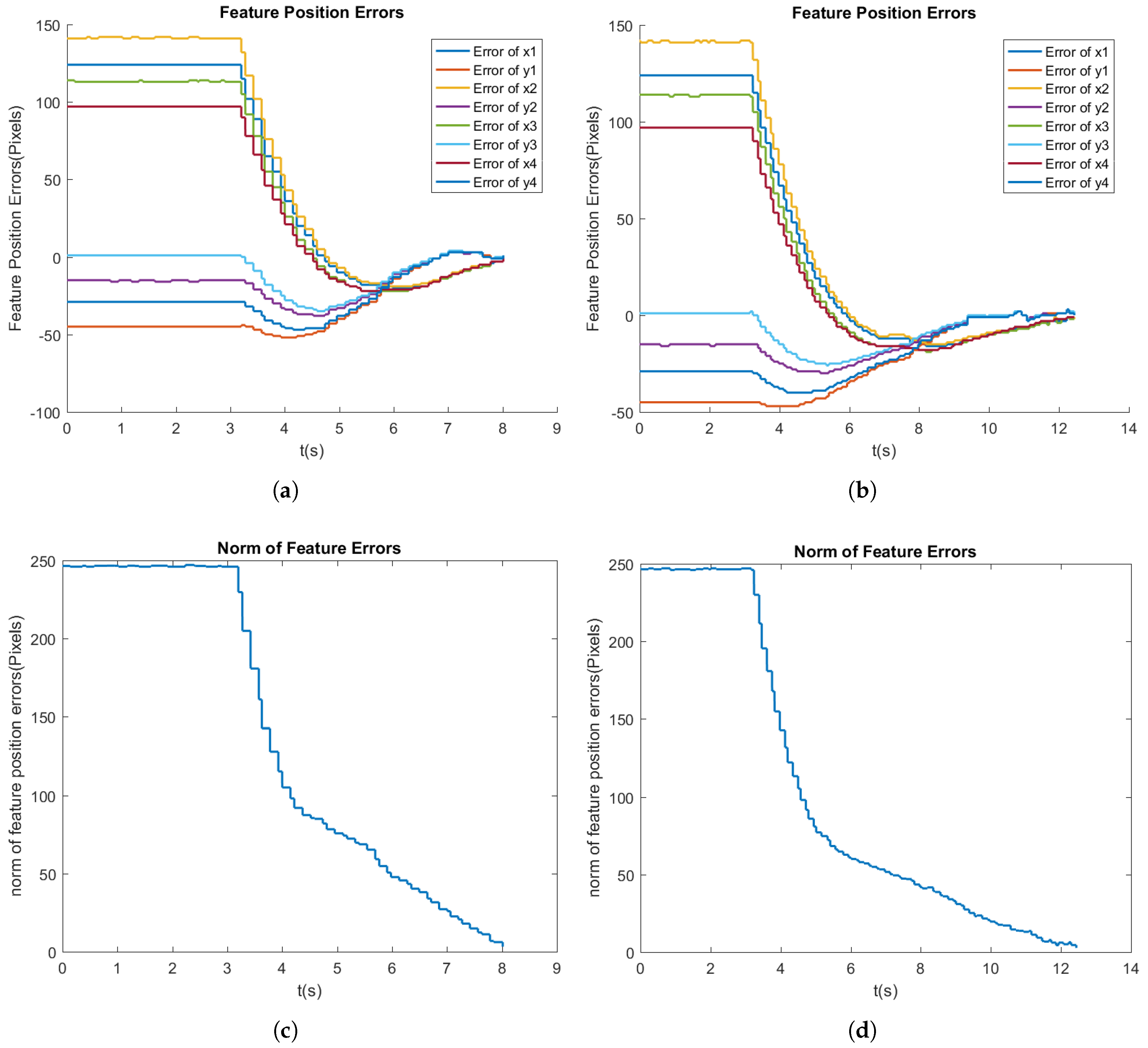
The task was to guide the end-effector to match the actual features with the desired ones in the camera image space. To simulate the condition where the features go outside FOV of the camera in real applications, the FOV of the camera was defined as the limited area shown in Figure 6a,b. When the features were in the defined FOV, they had actual position coordinates, and when they went outside FOV, the position coordinates of the features were set to zero. In this case, the proposed feature reconstruction algorithm was activated, and an estimate of the feature positions was generated. The norm of feature errors (NFE) is defined as below,

$$NFE=\sum _{n=1}^4\sqrt{{(x_n-x_{dn})}^2+{(y_n-y_{dn})}^2},$$

(23)

where $x_n$ and $y_n$ are the $n^{\mathrm{th}}$ feature coordinates and $x_{dn}$ and $y_{dn}$ are the $n^{\mathrm{th}}$ desired feature coordinates in the image plane.

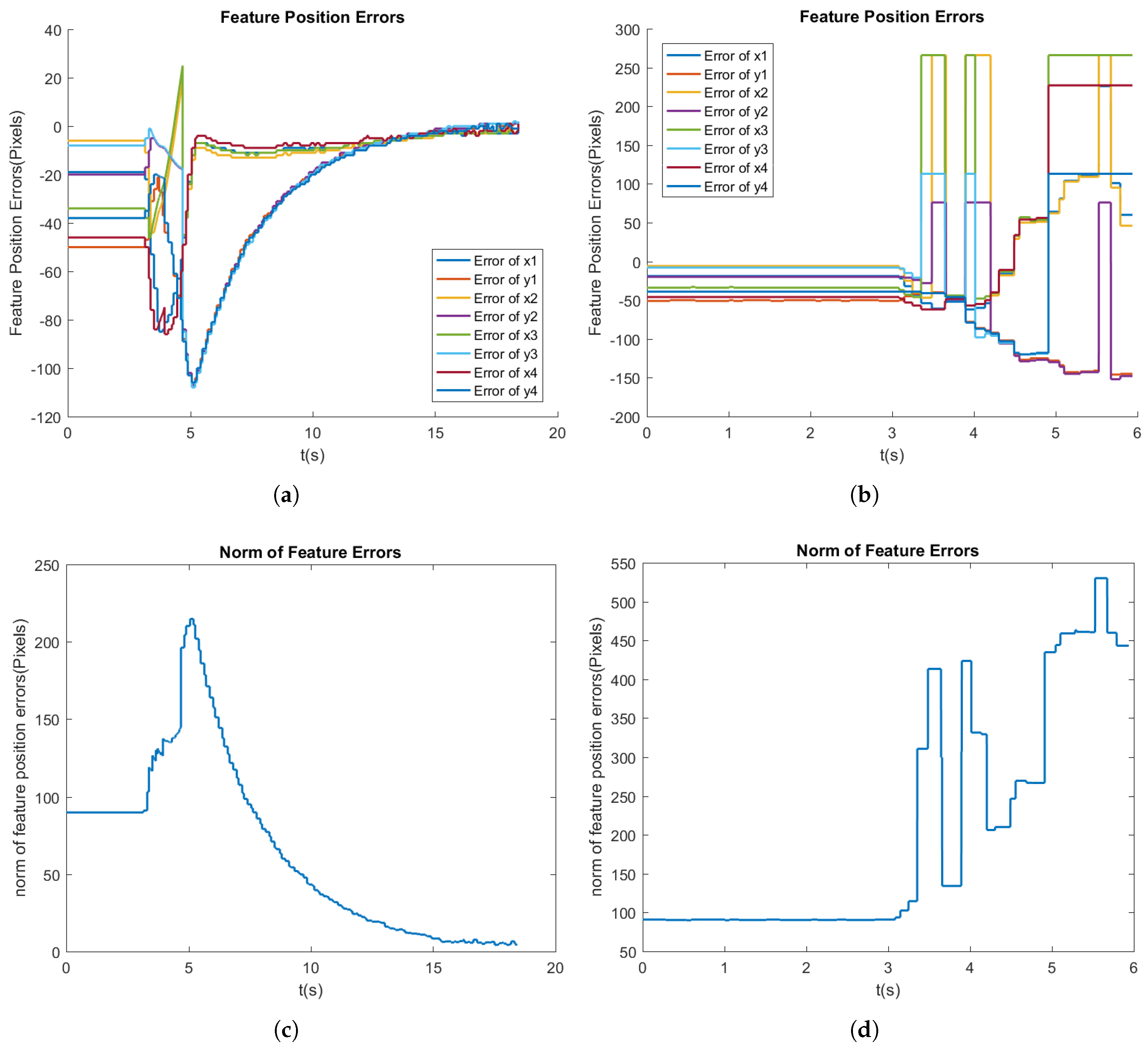
In the simulation test, we set the initial feature coordinates and the desired ones in a way that the image features were out of FOV. Figure 6 and Figure 7 demonstrate the performance comparison of the two methods. The paths of image features in the image space are given in Figure 6a,b. Figure 7a,b shows how the feature errors change with time in the proposed ESIBVSand switch method. Figure 7c,d demonstrates the norm of the feature errors’ change with time in both methods. As shown in the figures, ESIBVS was able to reduce the norm of the errors to the preset threshold, while in the switch method, the norm of the errors did not converge. The summary of the simulation test is shown in

Table 3. Test 1: Comparison of simulation results between ESIBVSand switch IBVS.

	Time of Convergence (s)		Final Norm of Feature Errors (Pixel)
	ESIBVS	Switch IBVS	ESIBVS	Switch IBVS
Test 1	12	Does not converge	1.5	Does not converge

. The results demonstrate how the proposed method was able to handle the situation in which the features went outside of the camera’s FOV and completed the task successfully, while the switch method was unable to do so.

6. Experimental Results

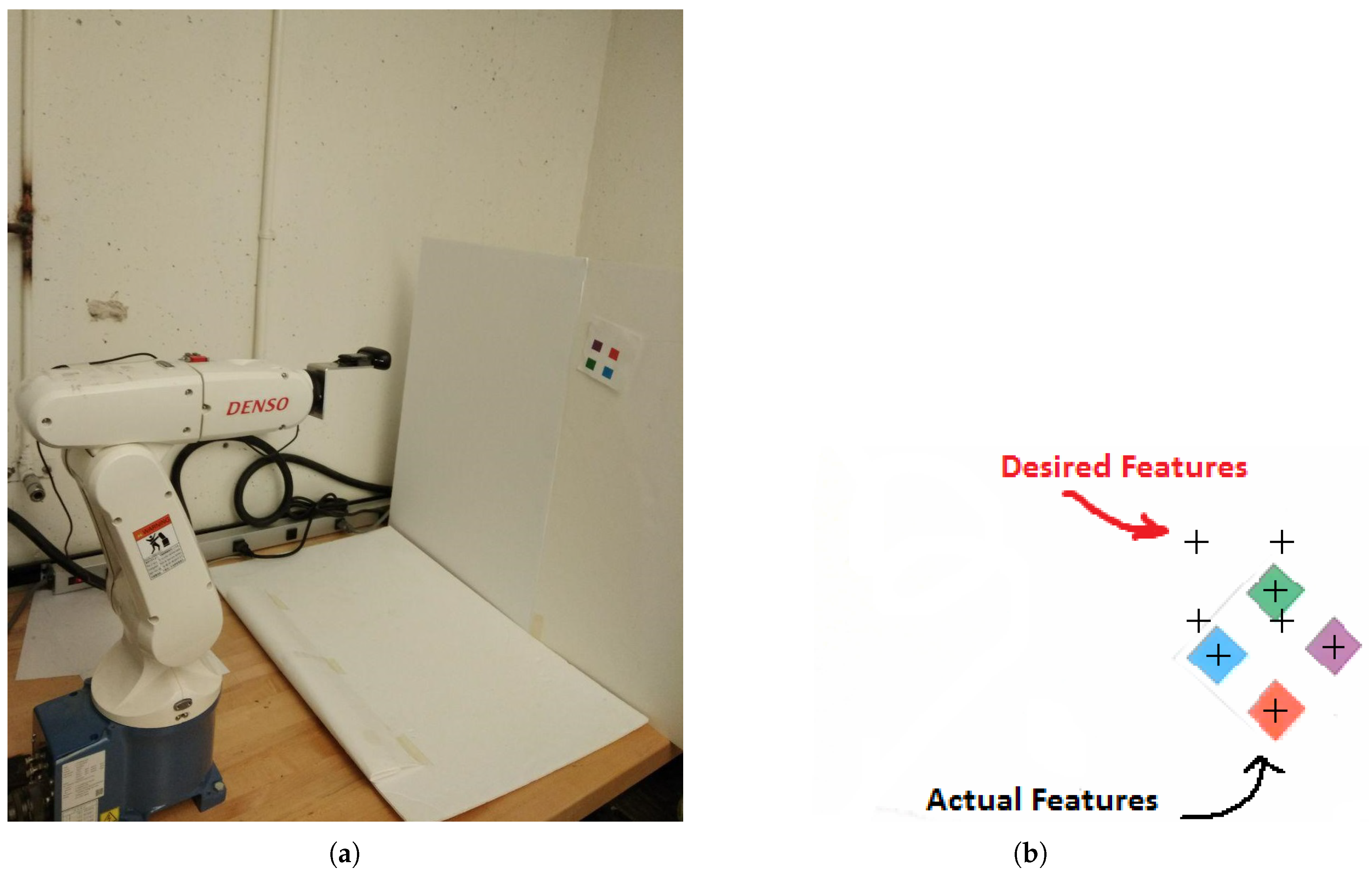
In this section, to further verify the effectiveness of the proposed method, some experiments were carried out, and the results are presented. The experimental testbed included a 6-DOF DENSOrobot with a camera (specifications shown in Table 2) installed on its end-effector (Figure 8a). The camera model was a Logitech Webcam HD 720p, which captures the video with a resolution of $1280\times 720$ pixels.

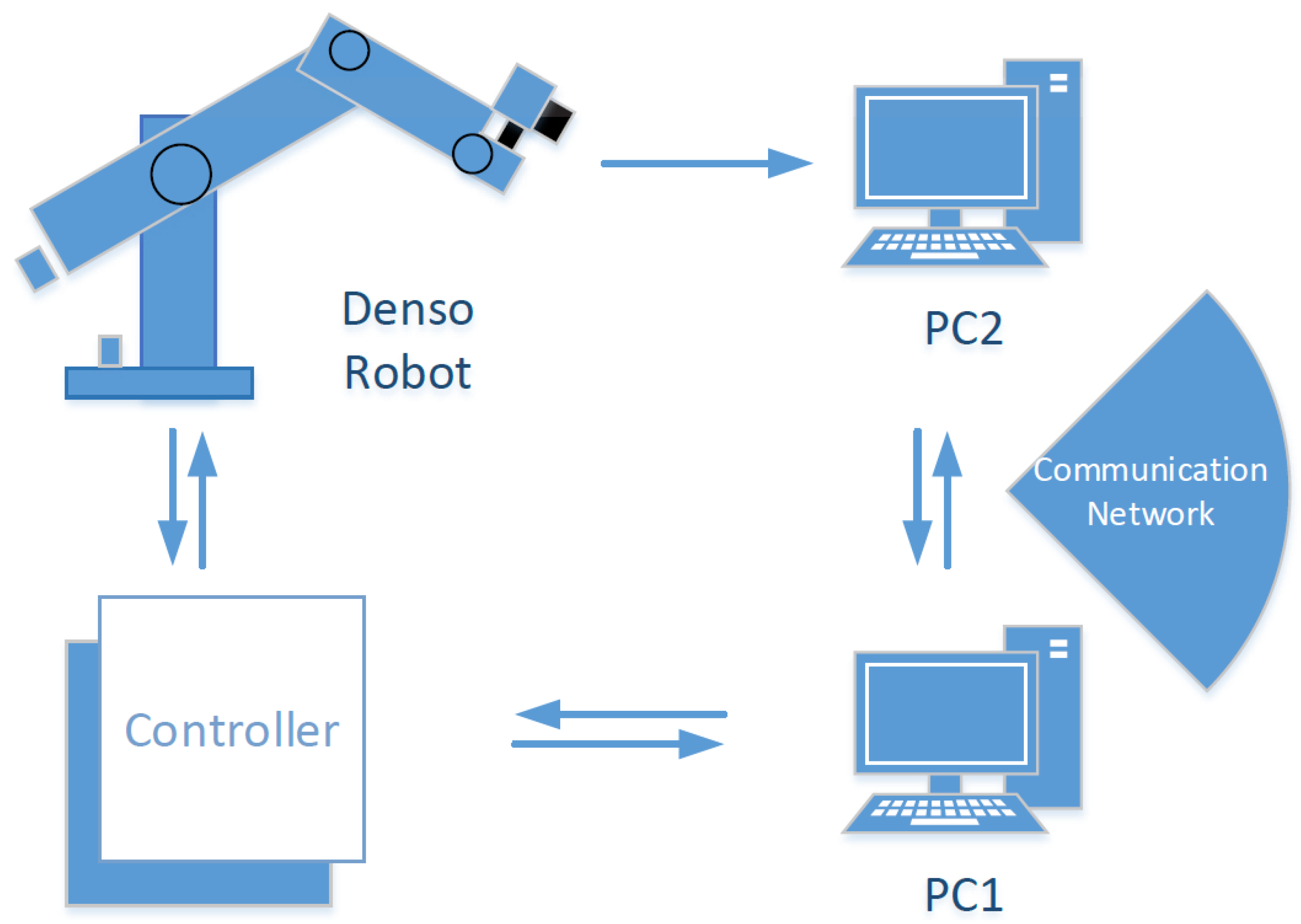
Two computers were used for the experimental tests. One computer carried out the image processing (PC2 in Figure 9) and sent the extracted feature coordinates to the other computer (PC1 in Figure 9), where the control algorithm was executed. Then, the control command (velocity of the end-effector) was sent to the robot controller. The image data taken by the camera were sent to an image processing program written by using the Computer Vision Toolbox of MATLAB. This program extracted the center coordinates of the features and sent them as feedback signals to the visual servoing controller in the sampling period of $0.001$ s. Four feature points were used in the control task. The detailed information of the image processing and feature extraction algorithm can be seen in our previous work [32]. The goal was to control the end-effector so that the actual features matched the desired ones (Figure 8b).

To evaluate the efficiency of ESIBVS, its performance was compared to that of the switch IBVS method. In all the tests, the threshold value of NFE was set to 0.005 (equivalent to four pixels). When NFE reached this value, the robot stopped, and the servoing task was fulfilled. The initial angle $\alpha$ between the actual and desired features (Figure 3) was ${50}^{\circ }$. $K_1$, $K_2$, and $K_3$ in (22) were set to 1, $0.4$, and $0.3$, respectively.

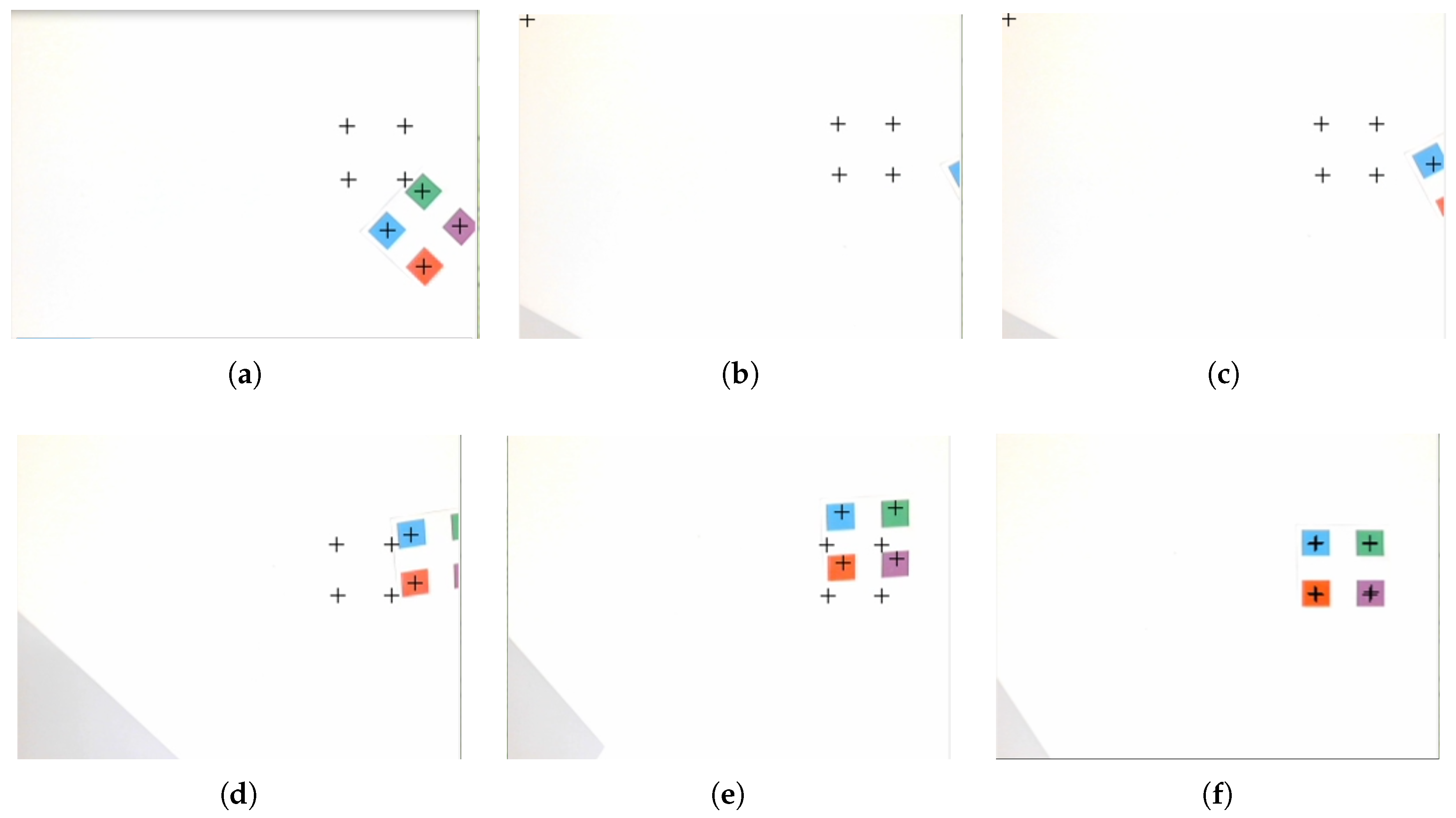
Test 2: In this test (The video can be found in the Supplementary Materials), the initial and desired features were set such that they went outside of the FOV of the camera during the test. The initial and desired feature coordinates in the test are given in

Table 4. Test 2: experiment, Initial (I) and desired (D) feature point positions in pixels.

		Point 1		Point 2		Point 3		Point 4
		(x, y)		(x, y)		(x, y)		(x, y)
Test 2	I	251	132	278	102	306	127	279	157
	D	232	82	272	82	272	119	233	119

. Figure 10 demonstrates the movement of actual features during the test of ESIBVS. It illustrates how the features went outside of FOV, then were reconstructed, went back to FOV, and finally matched the desired features.

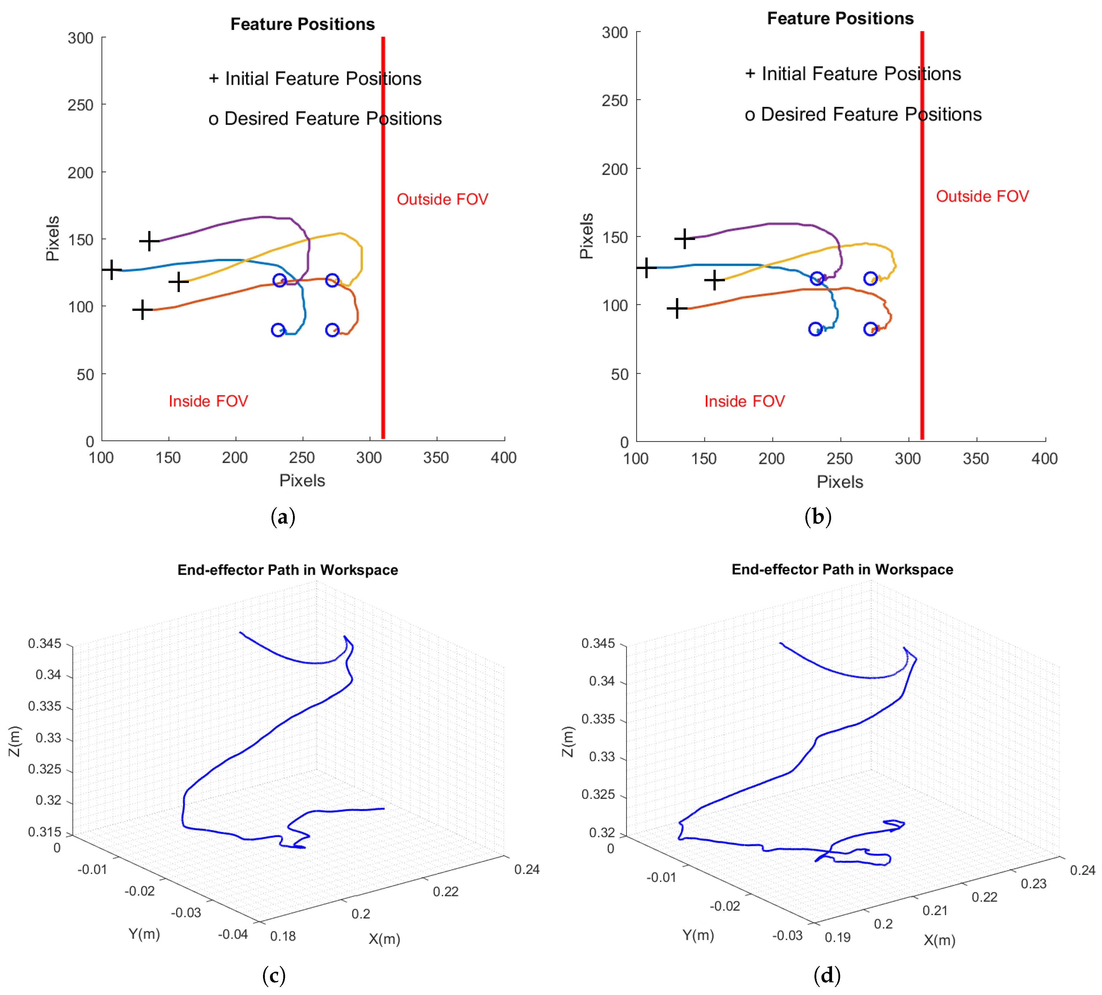
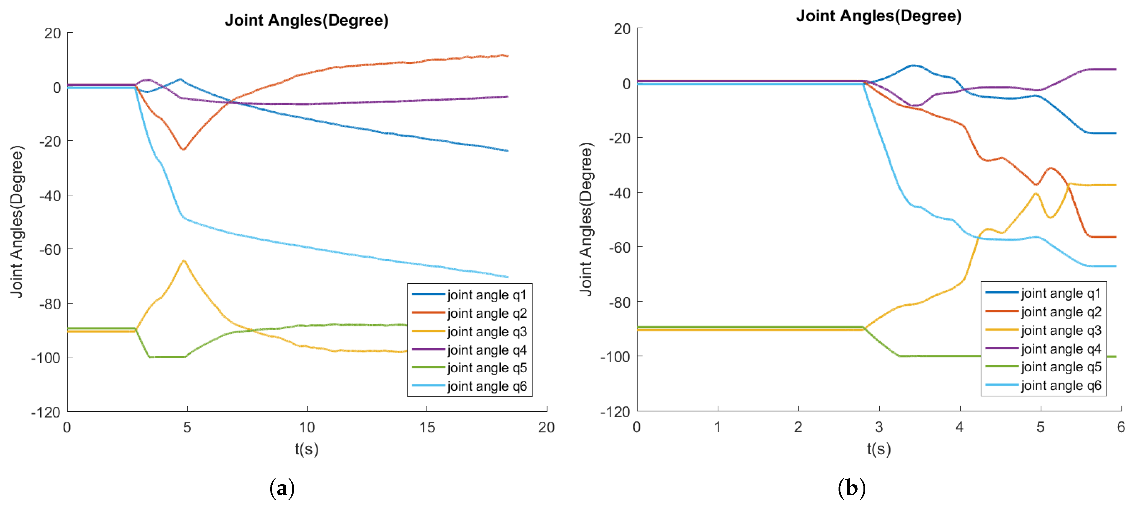
Figure 11, Figure 12 and Figure 13 show the comparison results between ESIBVS and switch IBVS. Figure 11 shows the paths of features in the image space from the initial positions to the desired ones, as well as the camera trajectory in Cartesian space. In the proposed method, the actual and desired features matched, while in switch IBVS, the actual features did not converge to the desired ones. Figure 12 demonstrates the robot joint angles in ESIBVS and switch IBVS. Figure 13 shows the comparison regarding the feature errors. The feature errors and the norm of feature errors in the proposed method successfully converged to the desired values (Figure 13a,c), while in the switch IBVS, the task could not be completed, and thus, the feature errors did not converge (Figure 13b,d).

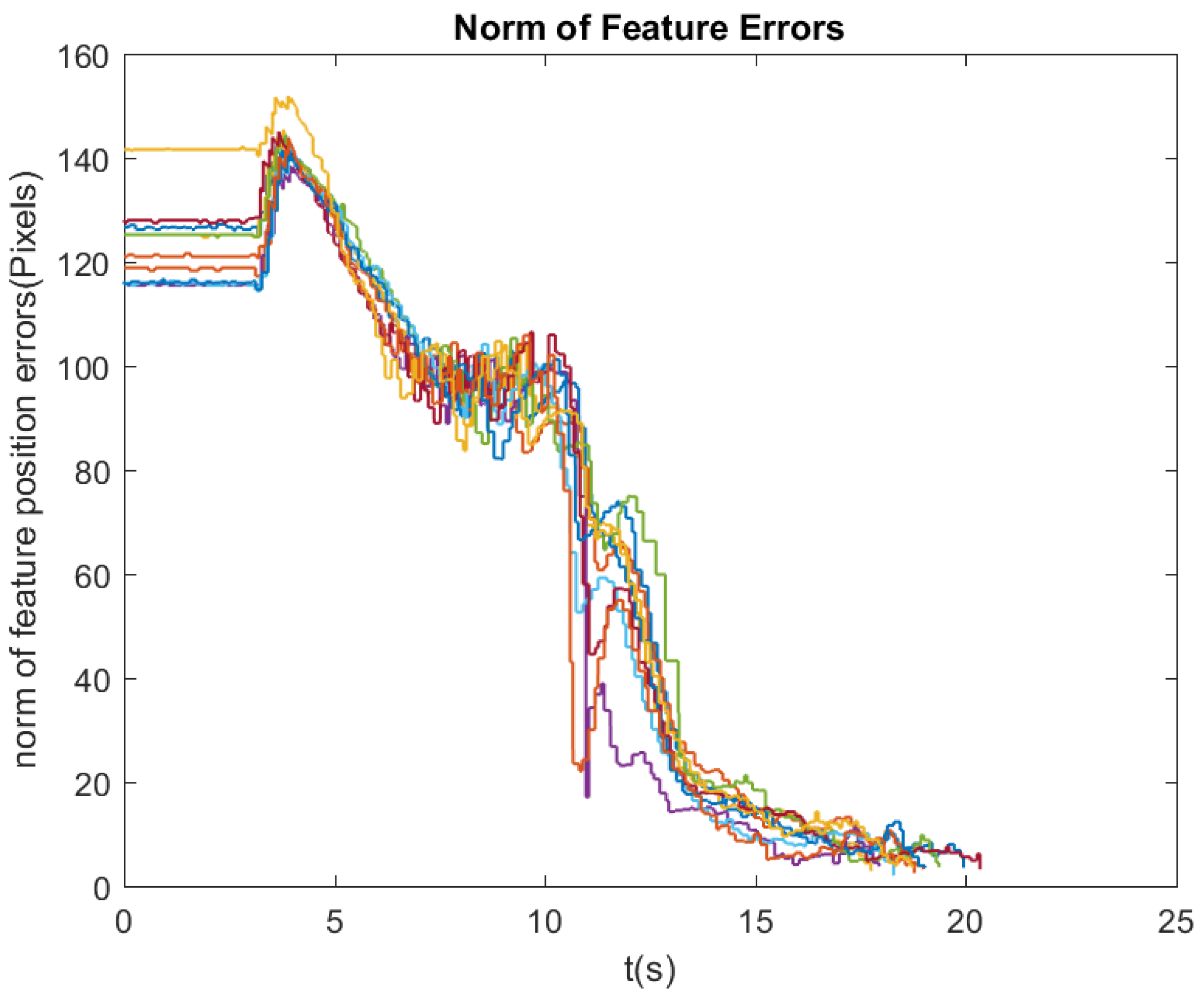
In order to further validate the performance of ESIBVS regarding the repeatability, the same test was repeated in 10 trials. The time of convergence and the final norms of feature error are shown in

Table 5. Test 2: experiment. Repeatability comparison results.

	Time of Convergence (s)		Final Norm of Feature Errors (Pixel)
	ESIBVS	Switch IBVS	ESIBVS	Switch IBVS
Trial 1	19.95	Does not converge	3.4	Does not converge
Trial 2	18.99	Does not converge	3.1	Does not converge
Trial 3	17.75	Does not converge	2.8	Does not converge
Trial 4	17.94	Does not converge	3.7	Does not converge
Trial 5	19.37	Does not converge	3.6	Does not converge
Trial 6	18.29	Does not converge	2	Does not converge
Trial 7	20.34	Does not converge	3.1	Does not converge
Trial 8	19.03	Does not converge	3.4	Does not converge
Trial 9	18.77	Does not converge	2.4	Does not converge
Trial 10	18.74	Does not converge	3.4	Does not converge

. The variations of feature error norms with time in 10 trials of ESIBVS are illustrated in Figure 14. As shown in the results, ESIBVS was able to overcome the feature loss and complete the task in each trial, while Switch IBVS was stuck in a point and did not converge.

Test 3: In this test, the performance of ESIBVS was compared with that of switch IBVS in the situation where the features did not leave the FOV of the camera. The initial and desired features were set in a way such that the features did not go outside of FOV (

Table 6. Test 3: Experiment. Initial (I) and desired (D) feature point positions in pixels.

		Point 1		Point 2		Point 3		Point 4
		(x, y)		(x, y)		(x, y)		(x, y)
Test 3	I	108	127	130	97	136	148	158	118
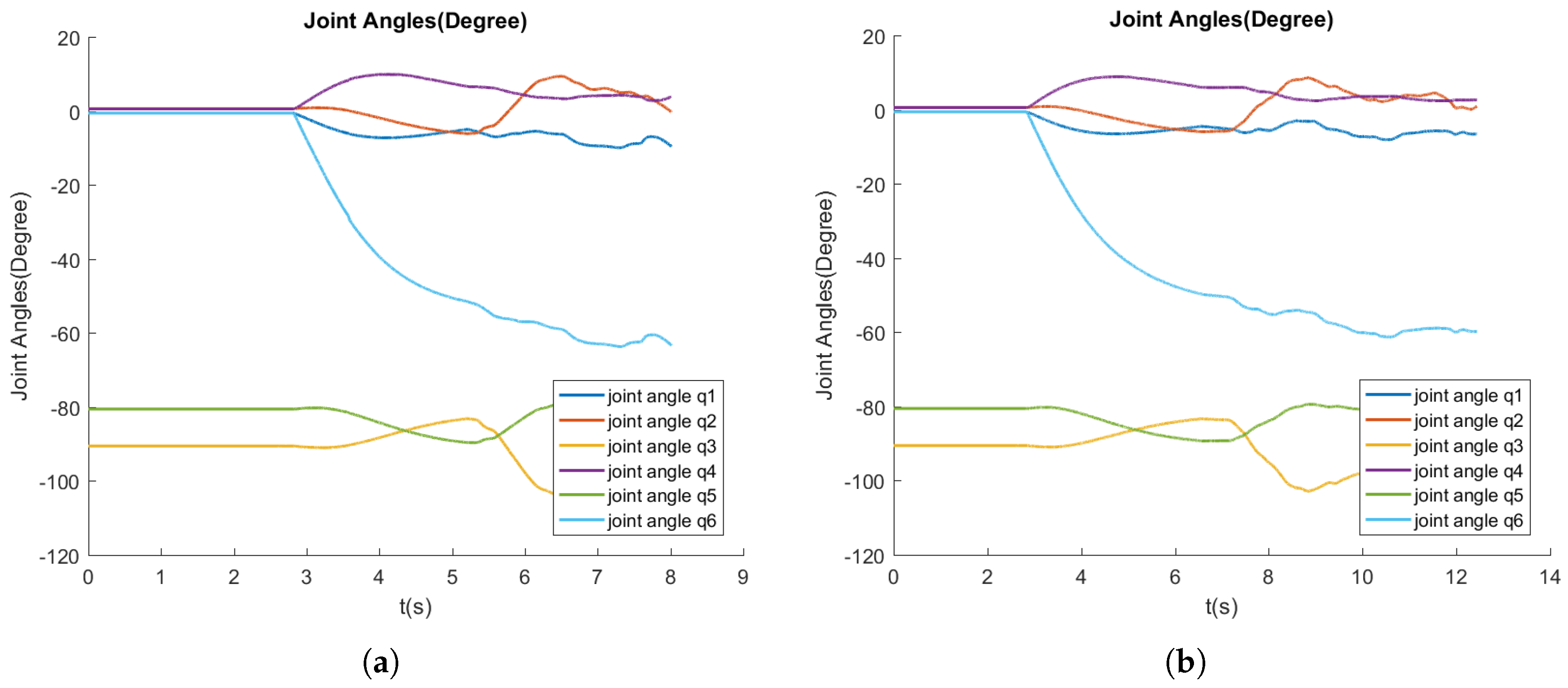
	D	232	82	272	82	272	119	233	119

). Similar to the previous tests, ESIBVS and switch IBVS were compared, and the results are shown in Figure 15, Figure 16 and Figure 17 and

Table 7. Test 3: Comparison of experimental resuts between ESIBVS and Switch IBVS.

	Time of Convergence (s)		Final Norm of Feature Errors (Pixel)
	ESIBVS	Switch IBVS	ESIBVS	Switch IBVS
Test 3	8	12.5	3.4	3.6

. As shown in the figures, ESIBVS had a $38\%$ shorter convergence time than switch IBVS did, which was owed to the superior noise-filtering ability of the designed Kalman filter.

The experimental results showed the efficiency of ESIBVS in dealing with feature loss while keeping the superior performance of the switch IBVS over traditional IBVS. As already shown in our previous work [15,16], the switch method was proven to have a better performance in its response time and its tracking performance, making it more feasible for industrial applications in comparison with the conventional IBVS. However, it suffered the drawback of weakness in dealing with feature loss. The proposed ESIBVS solved this problem and made switch IBVS more robust by using the Kalman filter to reconstruct the lost features.

7. Conclusions

This paper proposed an enhanced switch IBVS for a 6-DOF industrial robot. An image feature reconstruction algorithm based on the Kalman filter was proposed to handle feature loss during the process of IBVS. The combination of a three-stage switch controller and feature reconstruction algorithm improved the system response speed and tracking performance of IBVS and simultaneously overcame the problem of feature loss during the task. The proposed method was simulated and then tested on a 6-DOF robotic system with the camera installed in an eye-in-hand configuration. Both simulation and experimental results verified the efficiency of the method. In the future, we may extend the method to make it more robust to uncertainties such as the depth of features and camera parameters. In addition, the effect of different sampling periods on the performance of the proposed ESIBVS will be investigated.

References

1. Lee, Y.J.; Yim, B.D.; Song, J.B. Mobile robot localization based on effective combination of vision and range sensors. Int. J. Control Autom. Syst. 2009, 7, 97–104. [Google Scholar] [CrossRef]
2. Kim, J.H.; Lee, J.E.; Lee, J.H.; Park, G.T. Motion-based identification of multiple mobile robots using trajectory analysis in a well-configured environment with distributed vision sensors. Int. J. Control Autom. Syst. 2012, 10, 787–796. [Google Scholar] [CrossRef]
3. Banlue, T.; Sooraksa, P.; Noppanakeepong, S. A practical position-based visual servo design and implementation for automated fault insertion test. Int. J. Control Autom. Syst. 2014, 12, 1090–1101. [Google Scholar] [CrossRef]
4. Patil, M. Robot Manipulator Control Using PLC with Position Based and Image Based Algorithm. Int. J. Swarm Intell. Evol. Comput. 2017, 6, 1–8. [Google Scholar] [CrossRef]
5. Chaumette, F. Potential problems of stability and convergence in image-based and position-based visual servoing. In The Confluence of Vision and Control; Springer: London, UK, 1998; pp. 66–78. [Google Scholar] [Green Version]
6. Gans, N.R.; Hutchinson, S.A. Stable visual servoing through hybrid switched-system control. IEEE Trans. Robot. 2007, 23, 530–540. [Google Scholar] [CrossRef]
7. Malis, E.; Chaumette, F.; Boudet, S. 2 1/2 D visual servoing. IEEE Trans. Robot. Autom. 1999, 15, 238–250. [Google Scholar] [CrossRef] [Green Version]
8. Li, S.; Ghasemi, A.; Xie, W.F.; Gao, Y. An Enhanced IBVS Controller of a 6DOF Manipulator Using Hybrid PD-SMC Method. Int. J. Control Autom. Syst. 2018, 16, 844–855. [Google Scholar] [CrossRef]
9. Keshmiri, M.; Xie, W.F.; Ghasemi, A. Visual servoing using an optimized trajectory planning technique for a 4 DOFs robotic manipulator. Int. J. Control Autom. Syst. 2017, 15, 1362–1373. [Google Scholar] [CrossRef]
10. Keshmiri, M.; Xie, W.F. Image-based visual servoing using an optimized trajectory planning technique. IEEE/ASME Trans. Mechatron. 2016, 22, 359–370. [Google Scholar] [CrossRef]
11. Keshmiri, M.; Xie, W.F.; Mohebbi, A. Augmented image-based visual servoing of a manipulator using acceleration command. IEEE Trans. Ind. Electron. 2014, 61, 5444–5452. [Google Scholar] [CrossRef]
12. Kelly, R.; Carelli, R.; Nasisi, O.; Kuchen, B.; Reyes, F. Stable visual servoing of camera-in-hand robotic systems. IEEE/ASME Trans. Mechatron. 2000, 5, 39–48. [Google Scholar] [CrossRef] [Green Version]
13. Chen, J.; Dixon, W.E.; Dawson, M.; McIntyre, M. Homography-based visual servo tracking control of a wheeled mobile robot. IEEE Trans. Robot. 2006, 22, 406–415. [Google Scholar] [CrossRef] [Green Version]
14. Gans, N.R.; Hutchinson, S.A. A switching approach to visual servo control. In Proceedings of the 2002 IEEE International Symposium on Intelligent Control, Vancouver, BC, Canada, 30 October 2002; pp. 770–776. [Google Scholar]
15. Xie, W.F.; Li, Z.; Tu, X.W.; Perron, C. Switching control of image-based visual servoing with laser pointer in robotic manufacturing systems. IEEE Trans. Ind. Electron. 2009, 56, 520–529. [Google Scholar]
16. Ghasemi, A.; Xie, W.F. Decoupled image-based visual servoing for robotic manufacturing systems using gain scheduled switch control. In Proceedings of the 2017 International Conference on Advanced Mechatronic Systems (ICAMechS), Xiamen, China, 6–9 December 2017; pp. 94–99. [Google Scholar]
17. Hutchinson, S.; Hager, G.D.; Corke, P.I. A tutorial on visual servo control. IEEE Trans. Robot. Autom. 1996, 12, 651–670. [Google Scholar] [CrossRef]
18. Chaumette, F.; Hutchinson, S. Visual servo control. I. Basic approaches. IEEE Robot. Autom. Mag. 2006, 13, 82–90. [Google Scholar] [CrossRef]
19. Folio, D.; Cadenat, V. A controller to avoid both occlusions and obstacles during a vision-based navigation task in a cluttered environment. In Proceedings of the 44th IEEE Conference on Decision and Control, Seville, Spain, 15 December 2005; pp. 3898–3903. [Google Scholar]
20. Nicolis, D.; Palumbo, M.; Zanchettin, A.M.; Rocco, P. Occlusion-Free Visual Servoing for the Shared Autonomy Teleoperation of Dual-Arm Robots. IEEE Robot. Autom. Lett. 2018, 3, 796–803. [Google Scholar] [CrossRef]
21. Mezouar, Y.; Chaumette, F. Path planning for robust image-based control. IEEE Trans. Robot. Autom. 2002, 18, 534–549. [Google Scholar] [CrossRef]
22. Shen, T.; Chesi, G. Visual servoing path planning for cameras obeying the unified model. Adv. Robot. 2012, 26, 843–860. [Google Scholar]
23. Kazemi, M.; Gupta, K.K.; Mehrandezh, M. Randomized kinodynamic planning for robust visual servoing. IEEE Trans. Robot. 2013, 29, 1197–1211. [Google Scholar] [CrossRef]
24. Murao, T.; Yamada, T.; Fujita, M. Predictive visual feedback control with eye-in-hand system via stabilizing receding horizon approach. In Proceedings of the 2006 45th IEEE Conference on Decision and Control, San Diego, CA, USA, 13–15 December 2006; pp. 1758–1763. [Google Scholar]
25. Sauvée, M.; Poignet, P.; Dombre, E.; Courtial, E. Image based visual servoing through nonlinear model predictive control. In Proceedings of the 2006 45th IEEE Conference on Decision and Control, San Diego, CA, USA, 13–15 December 2006; pp. 1776–1781. [Google Scholar]
26. Lazar, C.; Burlacu, A.; Copot, C. Predictive control architecture for visual servoing of robot manipulators. In Proceedings of the IFAC World Congress, Milano, Italy, 28 August–2 September 2011; pp. 9464–9469. [Google Scholar]
27. Hajiloo, A.; Keshmiri, M.; Xie, W.F.; Wang, T.T. Robust online model predictive control for a constrained image-based visual servoing. IEEE Trans. Ind. Electron. 2016, 63, 2242–2250. [Google Scholar]
28. Assa, A.; Janabi-Sharifi, F. Robust model predictive control for visual servoing. In Proceedings of the 2014 IEEE/RSJ International Conference on Intelligent Robots and Systems (IROS 2014), Chicago, IL, USA, 14–18 September 2014; pp. 2715–2720. [Google Scholar]
29. Allibert, G.; Courtial, E.; Chaumette, F. Predictive control for constrained image-based visual servoing. IEEE Trans. Robot. 2010, 26, 933–939. [Google Scholar] [CrossRef]
30. García-Aracil, N.; Malis, E.; Aracil-Santonja, R.; Pérez-Vidal, C. Continuous visual servoing despite the changes of visibility in image features. IEEE Trans. Robot. 2005, 21, 1214–1220. [Google Scholar] [CrossRef]
31. Cazy, N.; Wieber, P.B.; Giordano, P.R.; Chaumette, F. Visual servoing when visual information is missing: Experimental comparison of visual feature prediction schemes. In Proceedings of the IEEE International Conference on Robotics and Automation (ICRA’15), Seattle, WA, USA, 26–30 May 2015; pp. 6031–6036. [Google Scholar]
32. Keshmiri, M. Image Based Visual Servoing Using Trajectory Planning and Augmented Visual Servoing Controller. Ph.D. Thesis, Concordia University, Montreal, QC, Canada, 2014. [Google Scholar]
Figure 1. Schematic of the camera model.
Electronics 08 00903 g001
Figure 2. Desired and initial feature positions inside and outside the camera’s field of view.
Electronics 08 00903 g002
Figure 3. Switch angle criteria α : the angle between the desired and actual features.
Electronics 08 00903 g003
Figure 4. Block diagram of the proposed enhanced switch image-based visual servoing (IBVS) controller.
Electronics 08 00903 g004
Figure 5. Flowchart of the Kalman filter feature reconstruction and control algorithm.
Electronics 08 00903 g005
Figure 6. Test 1: simulation. Image space feature trajectory comparison of enhanced switch IBVS and switch IBVS. (a) Image space feature trajectory in enhanced switch IBVS; (b) image space feature trajectory in switch IBVS.
Electronics 08 00903 g006
Figure 7. Test 1: simulation. Performance comparison of enhanced switch IBVS vs. switch IBVS. (a) Feature errors in enhanced switch IBVS; (b) feature errors in switch IBVS; (c) norm of feature errors in enhanced switch IBVS; (d) norm of feature errors in switch IBVS.
Electronics 08 00903 g007
Figure 8. (a) Experimental testbed, 6-DOF DENSO robot. (b) Actual and desired image features.
Electronics 08 00903 g008
Figure 9. Structure of the experimental testbed.
Electronics 08 00903 g009
Figure 10. Test 2: Snap shots of the camera image during the enhanced switch IBVS test: (a) Desired and actual feature positions at the start. (b) Actual features are out of FOV. (ce) Features are reconstructed and returned to FOV. (f) Final match of the desired and actual features.
Electronics 08 00903 g010
Figure 11. Test 2: experiment: Image space feature trajectory and 3D camera trajectory in enhanced switch IBVS and switch IBVS. (a) Image space feature trajectory in enhanced switch IBVS; (b) image space feature trajectory in switch IBVS; (c) camera 3D trajectory in enhanced switch IBVS; (d) camera 3D trajectory in switch IBVS.
Electronics 08 00903 g011
Figure 12. Test 2: experiment. Robot joint angles in enhanced switch IBVS and switch IBVS. (a) Joint angles (degree) in enhanced switch IBVS; (b) joint angles (degree) in switch IBVS.
Electronics 08 00903 g012
Figure 13. Test 2: experiment. Comparison of the feature errors and the norm of feature errors in enhanced switch IBVS and switch IBVS. (a) Feature errors in enhanced switch IBVS; (b) feature errors in switch IBVS; (c) norm of feature errors in enhanced switch IBVS; (d) norm of feature errors in switch IBVS.
Electronics 08 00903 g013
Figure 14. Test 2: experiment. The time variations of feature error norms in 10 trials of ESIBVS.
Electronics 08 00903 g014
Figure 15. Test 3: experiment. Image space feature trajectory and 3D camera trajectory in enhanced switch IBVS and switch IBVS. (a) Image space feature trajectory in enhanced switch IBVS; (b) image space feature trajectory in switch IBVS; (c) camera 3D trajectory in enhanced switch IBVS; (d) camera 3D trajectory in switch IBVS.
Electronics 08 00903 g015
Figure 16. Test 3: experiment. Robot joint angles in enhanced switch IBVS and switch IBVS. (a) Feature errors in enhanced switch IBVS; (b) feature errors in switch IBVS.
Electronics 08 00903 g016
Figure 17. Test 3: experiment. Comparison of feature errors and the norm of feature errors in enhanced switch IBVS and switch IBVS. (a) Feature errors in enhanced switch IBVS; (b) feature errors in switch IBVS; (c) norm of feature errors in enhanced switch IBVS; (d) norm of feature errors in switch IBVS.
Electronics 08 00903 g017