Dynamic Stress Measurement with Sensor Data Compensation

Abstract

Applying parachutes-deployed Wireless Sensor Network (WSN) in monitoring the high-altitude space is a promising solution for its effectiveness and cost. However, both the high deviation of data and the rapid change of various environment factors (air pressure, temperature, wind speed, etc.) pose a great challenge. To this end, we solve this challenge with data compensation in dynamic stress measurements of parachutes during the working stage. Specifically, we construct a data compensation model to correct the deviation based on neural network by taking into account a variety of environmental parameters, and name it as Data Compensation based on Back Propagation Neural Network (DC-BPNN). Then, for improving the speed and accuracy of training the DC-BPNN, we propose a novel Adaptive Artificial Bee Colony (AABC) algorithm. We also address its stability of solution by deriving a stability bound. Finally, to verify the real performance, we conduct a set of real implemented experiments of airdropped WSN.

1. Introduction

The wireless sensor network (WSN) has been studied more than one decade and provided mature solutions for surveillance and data collection from various fields, e.g., volcano, building, wild forest [1,2,3,4]. These applications have been well explored and studied. The application scenarios where surveillance targets vary rapidly and require high accuracy measurement in a high sampling rate, are still waiting for further exploration. For example, measuring dynamic stress of parachutes provides monitoring information for the entire process from opening to landing on the ground, which has a great significance not only on the development and production of new parachutes for various applications, but also on the safety of users.

In this paper, we mainly study the dynamic stress measurement of the parachute fabric and its specific applications. Specifically, we deploy our sensor components on parachutes to compose airdropped WSNs with dynamic pressure. However, such a sensor network still faces following challenges. First, during initial working process, shapes of parachutes and structures of networks change tremendously from the folded status to a fully open state. In addition, the sensor networks are affected by various environment factors like air pressure, temperature, wind movement which even would damage the equipment.

Thus, how to achieve acceptable measurement accuracy with ability-limited sensor networks in such rapid changing scenarios, which could be referred as dynamic measurement and data compensation problem in sensor networks, is still an open problem. Recently, various methods for sensor compensation have gradually attracted researchers’ attention because of its ability to reduce or eliminate the deficiency caused by error data on the systems [5,6,7,8,9,10,11,12,13]. For the compensation method of sensor data, most researches focus on hardware compensation based on physical or circuit characteristics of electronic components, such as magnetic field pulses, charge-coupled device, micro-electro-mechanical system, even material modification [6,7,8,9]. There are also a few high precision sensor methods with hardware and software compensation for temperature based on physical or circuit characteristics of the electronic elements [10,11]. Only a few works have focused on software compensation based on models or algorithms [12,13]. Compared to the latter one, the hardware method suffers from the drawbacks such as complex circuits, high cost, poor versatility, circuit drift and insufficient flexibility. As a result, we investigate how to build a more accurate model to achieve a better measurement performance in software compensation method rather than hardware deployment.

In this paper, we first combine the measured data (target characteristics) with the varied environmental factors (interference characteristics), such as temperature, humidity and wind speed, to construct a Data Compensation model based on Back Propagation Neural Network (DC-BPNN). Specifically, we adopt BPNN to minimize Mean Square Error (MSE) of the network through reversing propagation to adjust weights and thresholds [14,15]. Although there are many researches on BP-NN published, its learning algorithm has drawbacks like low efficiency, meanwhile, its solution is easy to fall into local optimal because of its non-convex hyper-surface of error surface [13]. All these limitations greatly affect the practical applications of BP-NN, especially under the complex environment. Hence, we introduce a heuristic algorithm—Artificial Bee Colony (ABC) [16] for parameter optimization. Furthermore, we proposed a novel algorithm named as Adaptive Artificial Bee Colony (AABC), which can adaptively select an appropriate path to optimize the parameters during the training process of DC-BPNN. In addition, we address the algorithm stability issue of AABC based on strict statistical analysis.

In summary, the contributions are listed as follows:

(1) We study the challenging and significant problem of dynamic fabric stress measurement of parachutes from opening to landing;

(2) Unlike other common approaches of hardware compensation or hydrodynamic simulated analysis, we propose a data analysis and compensation model—DCNN by considering both target and interference characteristics;

(3) To solve problems of local minimum solution and iterative redundancy, we propose a novel heuristic algorithm—AABC for the optimization of the weights and thresholds;

(4) We analyze the stability of our AABC in DC-BPNN model by strict statistical analysis techniques. To the best of our knowledge, there is few analysis or proof of algorithm stability of heuristic algorithms or evolutionary algorithms in published literatures.

2. Related Work

2.1. Sensor Data Compensation

In order to get the accurate data with sensors working in harsh environment, there are two methods in general: hardware compensation and soft compensation. The comparison of related compensation methods is listed in

Table 1. Comparison of hardware and software compensation methods for monitoring data in the WSN.

Methods of Compensation		Main Idea	Disadvantages	Speed	Accuracy
Hardware [5,6,7,8,9]		Use different complex circuits.	Costly, complex circuit, difficult to debug.	Fast	High
Software	Interpolation [17]	The ranges are segmented into pieces, and each segment is expressed by a polynomial.	The higher the accuracy is, the more storage space it needs.	Low	Depend on number of segments.
	LSPCF [18]	Find a matching function by minimizing the square of the error.	Ill-conditioned equations and long time-consumption caused by high order of fitted linear curves.	Medium	Medium
	BP-NN [19,20]	Minimize network error sum squares by feedback learning, with simpler implementation process.	Easy to fall into local optimal.	Fast	High

.

According to Table 1, the hardware compensation methods are generally expensive, complex, and difficult to debug and expand [5,6,7,8,9]. While, software compensation methods, including Interpolation [17], Least Square Polynomial Curve Fitting (LSPCF) [18] and BP neural network method [19,20], have obvious advantages as shown in Table 1. However, the Interpolation method requires large storage and needs to set the measurement range which is difficult to segment accurately, while LSPCF may generates odd or ill-conditioned equations because of the data fluctuation.

BP-NN is a powerful tool in data mining, which is prevailing for its characteristics such as parallel processing, distributed storage, self-learning, self-adaptive and high fault tolerance. Therefore, it has been widely used not only in many data mining fields, such as fitting, classification, prediction, pattern recognition, signal processing and image processing, but also in solving many system engineering problems because of its simply realization process and fast response speed [15,21]. Most importantly, it is also applied in the compensation system [19,20], which optimizes the neural network in different environments.

2.2. Heuristic Algorithms for BP Neural Network

However, from description in Introduction and Table 1, BP-NN have some disadvantages which restrict its applications [16]. In order to improve the efficiency of it, a heuristic method could solve it. In comparison with classical heuristic algorithms, Simulated Annealing (SA), which was inspired by solid annealing principle, has high complexity and unstable integration process [22]; Genetic Algorithm (GA) and Ant Colony Algorithm (ACG), which were inspired by simulation of nature evolution and imitation of foraging behavior of ants respectively, have complicated operations [23,24,25]; Particle Swarm Optimization (PSO), which was inspired by imitation of prey behavior of birds, has low complexity but complicated operation [25]; Artificial Bee Colony (ABC) algorithm, which simulated foraging paths behavior of a bee colony, has some advantages such as simpler operation, less parameters and stronger robustness [16].

Thus, in this paper, we further research how to improve the search habits and detection methods based on ABC algorithm for a faster and a more suitable search strategy in DC-BPNN.

2.3. Stress Measurements of Parachutes

With the rapid development of modern aerospace industry technology, parachutes, as a kind of the excellent airdrop recycling equipment, have always attracted high attention. Back in the 1970s, the United States and Russia have already begun to study on the stress measurement system of parachutes by some physics and fluid mechanics methods [26,27,28]. For stress measuring of parachutes during working process, many existing experimental methods are generally static experiments, rather than dynamic environments. Most works can only be carried out to measure the overall stress of fabric surface.

In recent years, with the rapid development of micro-electromechanical technologies, sensor and wireless communication technologies, there has been many successful applications by using low-power, low-cost and multi-functional sensors, which constitute a WSN to collect, transmit and calculate data [1,2,3,4]. Thus, WSN is ideal for dynamic measuring works here. However, according to the analysis in many aspects above in Introduction, there are some important challenges need to be solved, which are associated with the stress measurement and data compensation system of parachutes studied in this paper:

(1) How to deploy a suitable WSN on parachutes? How to measure the fabric stress dynamically?

(2) How to build a suitable data compensation model?

(3) How to optimize the model with required accuracy for the data compensation problem?

We will address discussions about the preceding questions in the following sections.

3. The Dynamic Measurement with Compensation System of Airdropped WSN

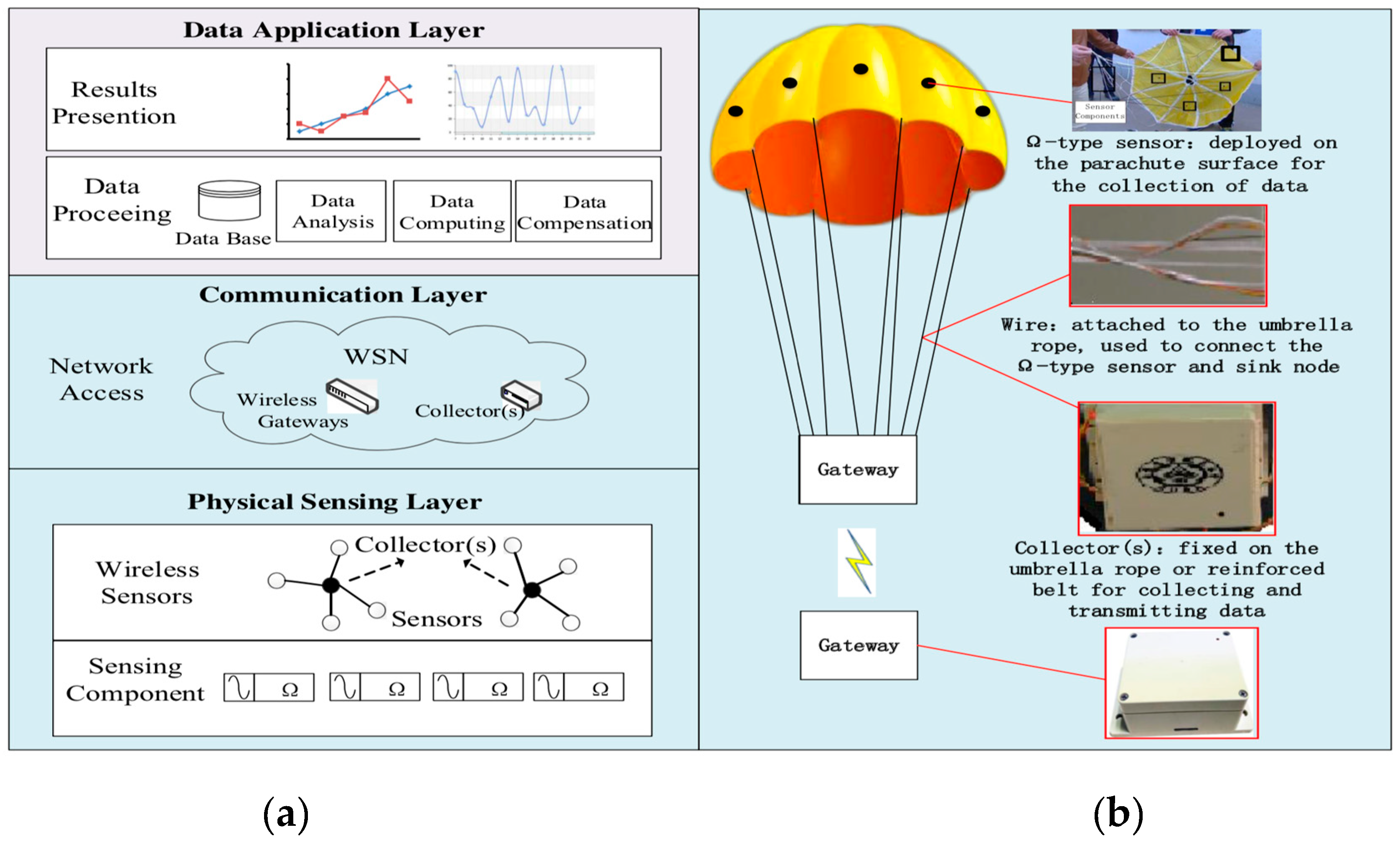
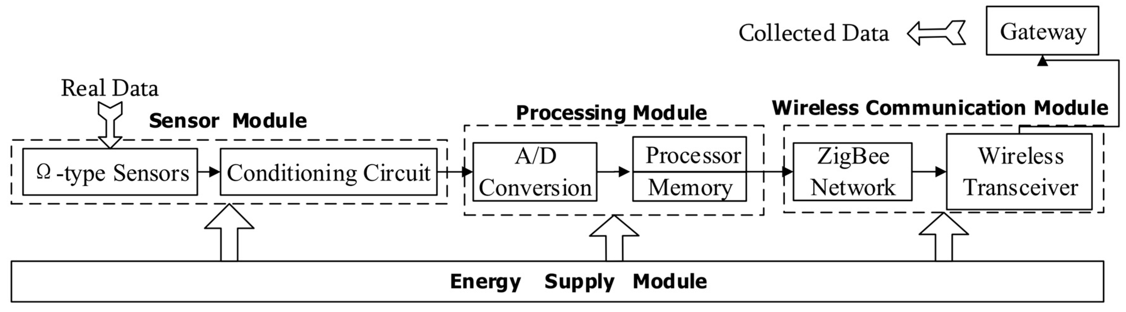
3.1. Network Structure and Deployment

The most important issue of parachutes is the safety and reliability, which highly relies on the limit of stress of its fabric. Thus, relevant researchers and manufacturers have paid particular attentions on the measurement of dynamic stress, especially in the opening status. In this paper, by deploying special sensor components developed by ourselves at various parts of parachutes’ surfaces, we can dynamically measure the fabric stress during their working process. However, when these devices are working in a high-altitude environment, they would be seriously affected by harsh weather conditions, which make parachutes’ shapes and structures change rapidly and some sensors could be detached. Therefore, we need to compensate the original collected data. Figure 1a shows the overall structure of our system based on airdropped WSN, which is composed of three functional layers: Physical sensing layer, network communication layer and data application layer.

In the physical sensing layer, sensors measure physical quantities during the process of airdrop. Considering the particularity of flexible fabric of parachutes, and in order to protecting the sensor circuit from being damaged or dropped by parachutes’ vibration or other environmental factors, we have designed a set of special Omega(Ω)-type sensor components [6]. Combining with other hardware auxiliary circuits, it can realize the real-time dynamical acquisition of data. Each sensor sends data to a collector, which aggregates and transmits the data to a gateway. The collected data can be stored at the gateway and transmitted to the ground control center. In the data application layer, the data process module preprocesses original data, compensate and associate data. Finally, it dynamically presents results in the top layer.

Figure 1b shows the implementation structures. Sensors are bonded to the surface of a parachute, connected with collectors via short wires. The collectors are deployed on parachute ropes and reinforcing belts. In this system, the sensor module includes gateway, collectors, the Ω-type on-chip stress sensors and their components. These sensors are small and light enough to be deployed directly on fabric surface [4].

Specifically, in the physical sensing layer, the main functions are data acquisition and transmission conversion. As shown in Figure 2, a collector is mainly composed of four parts: sensor module, processing module, wireless communication module and energy supply module. The working procedure is: First, in the sensor module, the stress information of a parachute’s flexible fabric is measured in the form of analog signal data by Ω-type sensors, then disposed and amplified by the conditioning circuit. Second, in the processing module, after A/D conversion, the collected information is packaged and transmitted by processors, and temporarily stored in the memory. Third, the wireless communication module is responsible for communication with other nodes, including ZigBee wireless networks and wireless transceivers. Meanwhile, the energy supply module typically uses miniature lithium batteries to provide energy to ensure the normal operation of nodes in the above modules. Specifically, as far as we know, it is difficult to measure directly the dynamic stress of flexible fabric. At present, the commonly used approach is measuring the electric voltages caused by the stress and converting the voltages to the stress values by using some methods [29], which will increase the uncertainty of results.

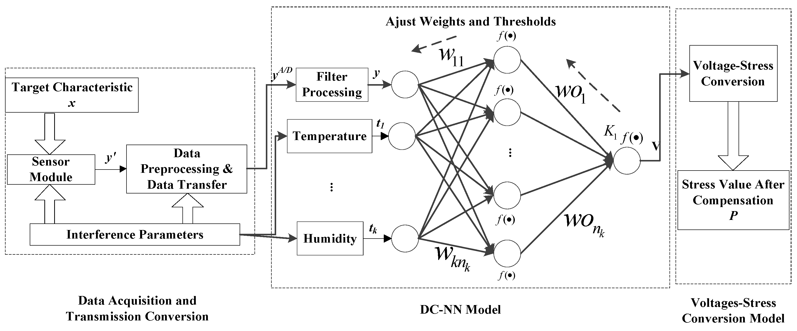
3.2. DC-BPNN Model Establishment

The data compensation framework is shown in Figure 3, including data acquisition and transmission conversion that has been described above, the DC-BPNN model and voltage-stress conversion model. In Figure 4, target characteristic $x$ is the actual voltage value to be measured. As aforementioned, $x$ is susceptible to interference feature parameters. y′ is the analog voltage. $y_j^{A/D}$ is the collected data from y′ converted by A/D conversion. We first remove the noise of sampled values through filter process to get y, as shown in Equation (1), where $\left\{y_j^{A/D}\right\}$ is a voltage sampling sequence measured by on-chip sensors, and $\left\{y_i\right\}$ is a voltage sequence after recursive filtering.

$$y_i=\frac{1}{n_k+1}{\displaystyle \sum _{j=i*n_k}^{\left(i+1\right)*n_k}}{y}_j^{\frac{A}{D}}$$

(1)

Here, the designed DC-BPNN model has three layers of neural network, including an input layer, an output layer, and a hidden layer. The number of the nodes in input layer is k + 1, including n input voltage $y=\left\{y_1,\cdots ,y_n\right\}$ in one node collected by the senor nodes. $t_1,t_2,\cdots ,t_k$ are k interference parameters in other k nodes, such as temperature, humidity, wind speed, atmospheric pressure. The number of nodes in hidden layer is $n_h$, and the number of nodes in the output layer is 1. $n_k$ is the number of extracting continuous sampling sequence. The input of DC-BPNN is $I=\left\{y_1,\cdots ,y_n,t_1,\cdots ,t_k\right\}=\left\{i{n}_1,\cdots ,i{n}_i,\cdots ,i{n}_{n+k}\right\}$, and the output is compensated voltage $V=\left\{v_1,\cdots ,v_i,\cdots ,v_n\right\}$. Then we can get the compensated stress value $P$ through the conversion of $V$ based on the voltage and stress mapping, which will be presented later.

The weight between the ith input layer node and the jth hidden layer node is marked as $w_{ij}$. The weight between the jth hidden layer node and the output layer node is marked as $w{o}_j$. The error accuracy is $\epsilon$ [14]. Here, we select the Sigmoid function as the excitation function to both the hidden layer and input layer, because it has the advantage of continuous and smoothness and a very good non-linear region to process both small value signals and large value signals [30]. Assuming that the lth input data in the ith node is $i{n}_l$, then the input hf(j) of the jth hidden layer node is calculated as shown:

$$hf\left(j\right)={\displaystyle {\sum }_{l=1}^{n+k}{w}_{ij}i{n}_l}-b_h$$

(2)

Here, $l\in \left[1,n+k\right],j\in \left[1,n_h\right]$. $b_h$ is the threshold of the hidden layer. From the Sigmoid function, the output hg(j) of the jth hidden layer node [12] is:

$$hg\left(j\right)=\frac{1}{1+e^{-hf\left(j\right)}}$$

(3)

Assuming the output value of the input layer mode is vf, $b_o$ is the threshold of the input layer [13], we have:

$$vf={\displaystyle {\sum }_{i=1}^{n_h}w{o}_{j}ho\left(j\right)}-b_o$$

(4)

From the Sigmoid function, the output value of the output layer can be calculated [13]:

$$V=\frac{1}{1+e^{-vf}}$$

(5)

The output voltage value and the expected value after compensation require an error calculation. If the node error is E, then:

$$E=\frac{1}{2}{\left(V-D\right)}^2$$

(6)

Here V is the output voltage after compensation, and D is the expected output voltage.

3.3. Voltage-Stress Conversion Model

We use a Temperature-Humidity-Material-Tensile-Testing (THMTT) machine to map the correspondence of voltages and stresses in a standard environment. Generally, we attach the sensor to the fabric sample to be tested, and the material to be tested is held vertically in the THMTT machine. Then, we measure the stress via the stress of materials. The stress changes both in radial and zonal directions. In order to study the impact of the elasticity of canopy fabric in the senor measurement, we carry out stress testing experiments on different sizes of the canopy fabric. This part of relevant detail research work has been published on [6]. Then, the voltage-stress conversion is:

$$\mathrm{F}={\displaystyle {\int }_0^{x_1}BS\left(v\right)ds}*\frac{x_2}{x_3}*\frac{q{\sigma }_{max}-\theta }{\sigma }$$

(7)

Here, $v$ is the voltage value collected by the sensor, $BS\left(v\right)$ is its corresponding stress value, and S is the cross-sectional area of the minizone fabric measured by an on-chip sensor. The notation $x_1$ is the fabric length of the measured area by an on-chip sensor, while $x_2$ is the corresponding width, and $x_3$ is the width of the whole sample fabric. $\frac{q{\sigma }_{max}-\theta }{\sigma }$ is the concentration factor of the stress. q is the distribution function. $\theta$ is the viscose impact factor, while $\sigma$ is the average stress, and ${\sigma }_{max}$ is the maximum stress. Assuming that the stress is evenly distributed in S, so the stress of the deployment area can be calculated by the integration of stress values in a small area.

4. Adaptive Artificial Bee Colony Algorithm IN DC-BPNN Model

For avoiding getting in a local optimal solution and iterative redundancy problem, we can train the DC-BPNN model by utilizing a heuristic stochastic search algorithm. Given strong optimization ability of ABC algorithm, we propose a novel AABC to find the optimal solution more accurately in DC-BPNN model.

4.1. Adaptive ABC--Improvement of Path Search

In ABC algorithm, each food source represents an associated solution of one optimization problem. Nectar amounts of a food source represent the fitness value of associated solutions, i.e., the qualities of the associated solutions. Bee’s honey mining process is similar to solve an optimization problem through the conversion, communication and collaboration between different bee roles [16]. (1) Employed bees: They search within the neighborhood of a food source. (2) Onlookers: They select a food source according to the shared food source information. (3) Scouts: When a food source has no update after several searches, it indicates that it has been caught in the local optimal.

A set of initial bee colony $x=\left\{x_1,x_2,\cdots ,x_{SN}\right\}$ with $SN$ solutions is randomly generated, where each solution (food source) $x_i\left(i=1,2,\cdots ,SN\right)$ is a d- dimensional vector. Generally, d is the number of optimization parameters. $S=\{(x_j^{min},x_j^{max})|j=(1,2,\cdots ,d)\}$, where $x_j^{min}$ and $x_j^{max}$ is the minimum and maximum value of the jth element in x. First, as in Equation (8), the food source is randomly determined [16]:

$$x_{ij}=x_j^{min}+rank\left(0,1\right)\left(x_j^{max}-x_j^{min}\right)$$

(8)

where, $x_{ij}$ indicates the jth component of the ith food source (that is, the ith associated solution), and j indicates the jth parameter to be optimized. $rank\left(0,1\right)$ indicates a random number between 0 and 1. Thereafter, employed bees will be assigned to the food source area to search for new food sources, and the location of the new food source is:

$$x_{ij}^{new}=x_{ij}+{\phi }_{ij}\left(x_{ij}-x_{kj}\right)$$

(9)

Here, $x_{kj}$ is a randomly selected food source, and j is the index of a randomly selected location. ${\phi }_{ij}$ controls the step length of searching a neighborhood food source, which is a random number in [−1,1]. When the newly searched food source (new associated solution) has more nectar amounts than the original one (old associated solution), the newer one will replace the older one. Specifically, we use the fitness (fit) of the food source to represent the nectar amounts [16], and $fi{t}_i\left(i=1,2,\cdots ,SN\right)$ to represent the fitness of each solution i, which can be calculated as:

$$fi{t}_i=\{\begin{array}{l}\frac{1}{1+f_i},f_i\ge 0\\ \frac{1}{abs\left(f_i\right)},f_i\ge 0\end{array}$$

(10)

Here, $f_i$ is the target function value of the ith associated solution. After all employed bees complete the search, scouts will select a food source according to nectar amounts proportional $p_i\left(i=1,2,\cdots ,SN\right)$ of the food source, which can be calculated by the Equation (11):

$$p_i=\frac{fi{t}_i}{{\sum }_{n=1}^{SN}fi{t}_n}$$

(11)

Scouts select a food source according to the nectar amounts proportional $p_i$ of each honey source and select a more optimal food source to search. Then a new food source $x_i^{new}$ is generated by Equation (9). If the fitness is higher than the current food source, then it is replaced by the newer one $x_i^{new}$.

According to the above description, we can find that Equation (9) will be used repeatedly in the process of searching for new food sources. However, the step length factor ${\phi }_{ij}$ controls the search of food sources is a random number on [−1,1] and does not take advantage of any prior information, which not only reduces the accuracy of the ${\phi }_{ij}$ value, but also makes it easy to increase the calculating time. Thus, we can make an improvement on the selection of ${\phi }_{ij}$ value, and propose the Adaptive ABC (AABC) algorithm.

Intuitively, if a food source had a higher nectar amount, the quality of the associated solution near the food source would be higher and might even contain the optimal solution. And if a food source has a very lower nectar amounts proportional, which means that the quality of the associated solution is low and employed bees need to continue searching in a further area to find a better source with higher quality. Therefore, according to Equation (11), if a food source has a higher nectar amounts proportional in the previous search, the step length factor should be smaller in a new search and scouts only need to find food sources nearby. That is, the larger the $p_i$ value is ($p_i\in \left(0,1\right)$), the greater chance it might find to present the optimal solution, and the smaller the step length should be. Therefore, we modify Equation (9), and a new food source is generated through Equation (12):

$$x_{ij}^{new}=x_{ij}+{\omega }_{ij}\left(x_{ij}-x_{kj}\right)$$

(12)

Here, ${\omega }_{ij}$ is the new step length factor, which can be calculated as follows:

$${\omega }_{ij}=\{\begin{array}{c}rand\left\{\left[-1,-0.5\right]\cup \left[0.5,1\right]\right\},p_i\le 0.5\\ rand\left[-p_i,p_i\right],p_i>0.5\end{array}$$

(13)

Through the cooperation of bees, AABC tends to converge after repeated iterations, and obtain the optimal solution or the approximate optimal solution of the problem in the associated solution space. Generally speaking, the quantities of employed bees and scouts are the same, so their quantity equals to the quantity of solutions. If employed bees still cannot improve the quality of the solution after trying for given times, they will become scouts. They randomly search a new possible food source (that is, a new associated solution) in the area, and start a new search. The original solution will be abandoned. Trying times is named as abandonment criteria, representing by $C_{max}$.

4.2. Stability of AABC Algorithm in DC-BPNN Model

According to the above analysis, we conclude corresponding relations of parameters in AABC algorithm and DC-BPNN model, which is shown in

Table 2. Corresponding relations between the AABC and DC-BPNN.

AABC	DC-BPNN
Colony size	Solution quantity
Food source quality (Fitness)	MSE
Speed of searching the best food source	Speed of optimization
Best food source	Global optimal solution
Food source dimension	Neural network dimension

.

When training the DC-BPNN, we generally use MSE between the network output and the expected output as the target optimal function as shown in Equation (6). The key of training our DC-BPNN is to find a set of weight and threshold to minimize the MSE. From Table 2, we can find that features in DC-BPNN have their corresponding parameters in AABC. Next, we will analysis the stability of our AABC in DC-BPNN.

Algorithmic stability is a notion in computational learning theory of how an algorithm is perturbed by small changes to its inputs, which can guarantee that the learning algorithm will generalize on new examples [31]. A stable learning algorithm is one for which the prediction does not change much when the training data is modified slightly. Therefore, in order to prove that our AABC is stable, we analyze the output of the algorithm on two data sets that differ in precisely one location. Specifically, stability analysis calculates generalization bounds for supervised learning algorithms [32]. Formally, the learning problem here is specified by the sample $I=\left[i{n}_1,\cdots ,i{n}_i,\cdots ,i{n}_{n+k}\right]\in R^{n_p\times \left(n+k\right)}$ of $\left(n+k\right)$ examples and an objective loss function $f$, which is just the fitness function determining the quality of solutions. Generally, the function $f$ are selected from a hypothesis space $\mathscr{H}$. The sample $I$ is drawn i.i.d. from a distribution $\mathcal{D}$. The quality of each hypothesis $h\in \mathscr{H}$ is measured by its population risk:

$$\mathrm{F}\left[h\right]\stackrel{def}{=}{\mathrm{E}}_{in\sim \mathcal{D}}f\left(h;s\right)$$

(14)

Here, $f\left(h,is\right)$ designates the loss of the model described by $f$ on the example $s$ [32]. $\mathbb{E}$ is the expectation. Ideally, the risk of $h\in H$ is as close as possible to infimum of $F\left[h\right]$. However, we can not estimate it directly, we characterize the empirical risk of $f$ to instead of the Equation (14):

$${\mathrm{F}}_e\left[h\right]\stackrel{def}{=}\frac{1}{n+k}{\displaystyle \sum _{i=1}^{n+k}}f\left(h;i{n}_i\right)$$

(15)

Thus, we can obtain an expected generalization error with rate $\epsilon \left(n+k\right)$ under distribution $\mathcal{D}$ if for all of $\left(n+k\right)$ samples:

$$E_{I\sim {\mathcal{D}}^{n+k}}\left[\mathrm{F}\left[h\right]-{\mathrm{F}}_e\left[h\right]\right]\le \epsilon \left(n+k\right)$$

(16)

Let mapping $A:{\cup }_{i\in I}{I}^{n+k}\to H$, and $h=A\left(I\right)$ [31]. Then, from Equation (16), we can get:

$$E_{\mathrm{I}\sim {\mathcal{D}}^{\mathrm{n}+\mathrm{k}}}\left[\mathrm{F}\left[\mathrm{A}\left(I\right)\right]-{\mathrm{F}}_e\left[\mathrm{A}\left(I\right)\right]\right]\le \epsilon \left(n+k\right)$$

(17)

Since we try to analyze the stability of our AABC, i.e., verify the algorithm are stable by slight changes from different inputs, we denote two independent samples $I=\left[i{n}_1,\dots ,i{n}_i,\dots i{n}_{n+k}\right]$, and $I^{\prime }=\left[i{n}_1^{\prime },\dots ,i{n}_i^{\prime },\dots i{n}_{n+k}^{\prime }\right]$. For any $i$, both $i{n}_i$ and $i{n}_i^{\prime }$ are drawn i.i.d form the distribution $\mathcal{D}$. Let $I^{\left(i\right)}=\left[i{n}_1,\dots ,i{n}_{i-1},i{n}_i^{\prime },i{n}_{i+1},\dots i{n}_{n+k}\right]$ be a sample where the $ith$ data equals to $i{n}_i^{\prime }$ in sample $I^{\prime }$ and the rest data are the same as ones in the sample $I$. Hence, we have that:

$$\begin{array}{cc}\hfill E_{I\sim {\mathcal{D}}^{n+k}}\left[{\mathrm{F}}_e\left[\mathrm{A}\left(I\right)\right]\right]& =E_{I\sim {\mathcal{D}}^{n+k}}\left[\frac{1}{n+k}{\displaystyle \sum _{i=1}^{n+k}}f\left(\mathrm{A}\left(I\right);i{n}_i\right)\right]\hfill \\ & =\frac{1}{n+k}{\displaystyle \sum _{i=1}^{n+k}}{E}_{I\sim {\mathcal{D}}^{n+k}}\left[f\left(\mathrm{A}\left(I\right);i{n}_i\right)\right]\hfill \\ & =\frac{1}{n+k}{\displaystyle \sum _{i=1}^{n+k}}{E}_{I\sim {\mathcal{D}}^{n+k}}{E}_{{in}_i^{\prime }\sim \mathcal{D}}\left[f\left(\mathrm{A}\left(I^i\right);{in}_i^{\prime }\right)\right]\hfill \end{array}$$

(18)

For simplicity, we denote ${\mathrm{E}}_I\left[\mathrm{F}\left[\mathrm{A}\left(I\right)\right]={\mathrm{E}}_{I\sim {\mathcal{D}}^{n+k}}\right[\mathrm{F}\left[\mathrm{A}\left(I\right)\right]$. With the Equation (18), we can rewrite the expected generalization error:

$$\begin{array}{cc}\hfill E_I{E}_A\left[{\mathrm{F}}_{\mathrm{e}}\left[\mathrm{A}\left(I\right)\right]\right]& =E_I{E}_A\left[\frac{1}{n+k}{\displaystyle \sum _{i=1}^{n+k}}f\left(\mathrm{A}\left(I\right);i{n}_i\right)\right]\hfill \\ & =E_{I^{\prime }}{E}_I{E}_A\left[\frac{1}{n+k}{\displaystyle \sum _{i=1}^{n+k}}f\left(\mathrm{A}\left(I^{\left(i\right)}\right);{in}_i^{\prime }\right)\right]\hfill \\ & =E_{I^{\prime }}{E}_I{E}_A\left[\frac{1}{n+k}{\displaystyle \sum _{i=1}^{n+k}}f\left(\mathrm{A}\left(I^{\left(i\right)}\right);{in}_i^{\prime }\right)\right]\hfill \\ & =E_{I^{\prime }}{E}_{I}E\left[\frac{1}{n+k}{\displaystyle \sum _{i=1}^{n+k}}f\left(\mathrm{A}\left(I\right);{in}_i^{\prime }\right)\right]\hfill \\ & +E_{I^{\prime }}{E}_I{E}_A\left[\frac{1}{n+k}{\displaystyle \sum _{i=1}^{n+k}}\left[f\left(\mathrm{A}\left(I^{\left(i\right)}\right);{in}_i^{\prime }\right)-f\left(\mathrm{A}\left(I\right);{in}_i^{\prime }\right)\right]\right]\hfill \\ & =E_I{E}_A\left[F\left[\mathrm{A}\left(I\right)\right]\right]\hfill \\ & +E_{I^{\prime }}{E}_I{E}_A\left[\frac{1}{n+k}{\displaystyle \sum _{i=1}^{n+k}}\left[f\left(\mathrm{A}\left(I^{\left(i\right)}\right);{in}_i^{\prime }\right)-f\left(\mathrm{A}\left(I\right);{in}_i^{\prime }\right)\right]\right]\hfill \end{array}$$

(19)

Thus, the generalization error of AABC is:

$$\left|E_{I,A}\left[F_e\left[A\left(I\right)\right]\right]-E_{I,A}\left[\mathrm{F}\left[\mathrm{A}\left(I\right)\right]\right]\right|=\left|E_{I^{\prime }}{E}_I{E}_A\left[\frac{1}{n+k}{\displaystyle \sum _{i=1}^{n+k}}\left[f\left(\mathrm{A}\left(I^{\left(i\right)}\right);{in}_i^{\prime }\right)-f\left(\mathrm{A}\left(I\right);{in}_i^{\prime }\right)\right]\right]\right|$$

(20)

According to average-RO stable rule [33], we have:

$$\left|E_{I^{\prime }}{E}_I{E}_A\left[\frac{1}{n+k}{\displaystyle \sum _{i=1}^{n+k}}\left[f\left(\mathrm{A}\left(I^{\left(i\right)}\right);{in}_i^{\prime }\right)-f\left(\mathrm{A}\left(I\right);{in}_i^{\prime }\right)\right]\right]\right|\le {\epsilon }_{stable}\left(n+k\right)$$

(21)

So, Equation (20) can be rewrite as:

$$\left|E_{I,A}\left[{\mathrm{F}}_{\mathrm{e}}\left[\mathrm{A}\left(I\right)\right]-E_{I,A}\right[\mathrm{F}\left[\mathrm{A}\left(I\right)\right]\right|\le {\epsilon }_{stable}\left(n+k\right)$$

(22)

From Equation (10), we can know the fitness function is non-convex, thus

$${\epsilon }_{stable}\left(n+k\right)<\approx \frac{T^{1-1/\left(\beta c+1\right)}}{n+k}$$

(23)

where, T is the steps of solving solution, $\beta$ is the factor of $\beta$-smooth and $c$ is the step factor [32], which both are positive. Obviously, $T^{1-1/\left(\beta c+1\right)}$ is less than $T$, and generally $\left(n+k\right)$ ≫ T, then we have:

$$\underset{\left(n+k\right)\to \infty }{\lim }\frac{T^{1-1/\left(\beta c+1\right)}}{n+k}=0$$

(24)

As a result, the generalization error of our AABC is slight, which means its uniformly stable on another new similar scene.

5. Experiments

In order to verify the effectiveness of our method, we perform different types of experiments. First, we training the DC-BPNN model from the training data collected by the Temperature-Humidity-Material-Tensile-Testing (THMTT) machine experiment. In this phase, we estimate the mapping between the stress value (within different stress ranges) and the voltage value under different temperatures and humidity by the THMTT machine. Second, we verify the effectiveness in a real airdropped environment. Third, for verifying a better optimization result of our AABC, we also compare our AABC with ABC and the Levenberg-Marquardt (LM) [34], which is a common method for solving optimal solution.

The experimental sensors are the $\Omega$-type on-chip sensors [6]. The collector of this work uses the CC2530 wireless communication module, which is a ZigBee-based system-on-chip. In our work, the sampling frequency is 2 K/s and 2 bytes in one sampling. The general duration of an airdrop experiment is about 2 h. About the software design, we apply 4 KB memory space as a buffer for sending data and apply > 4 KB memory space for storing data.

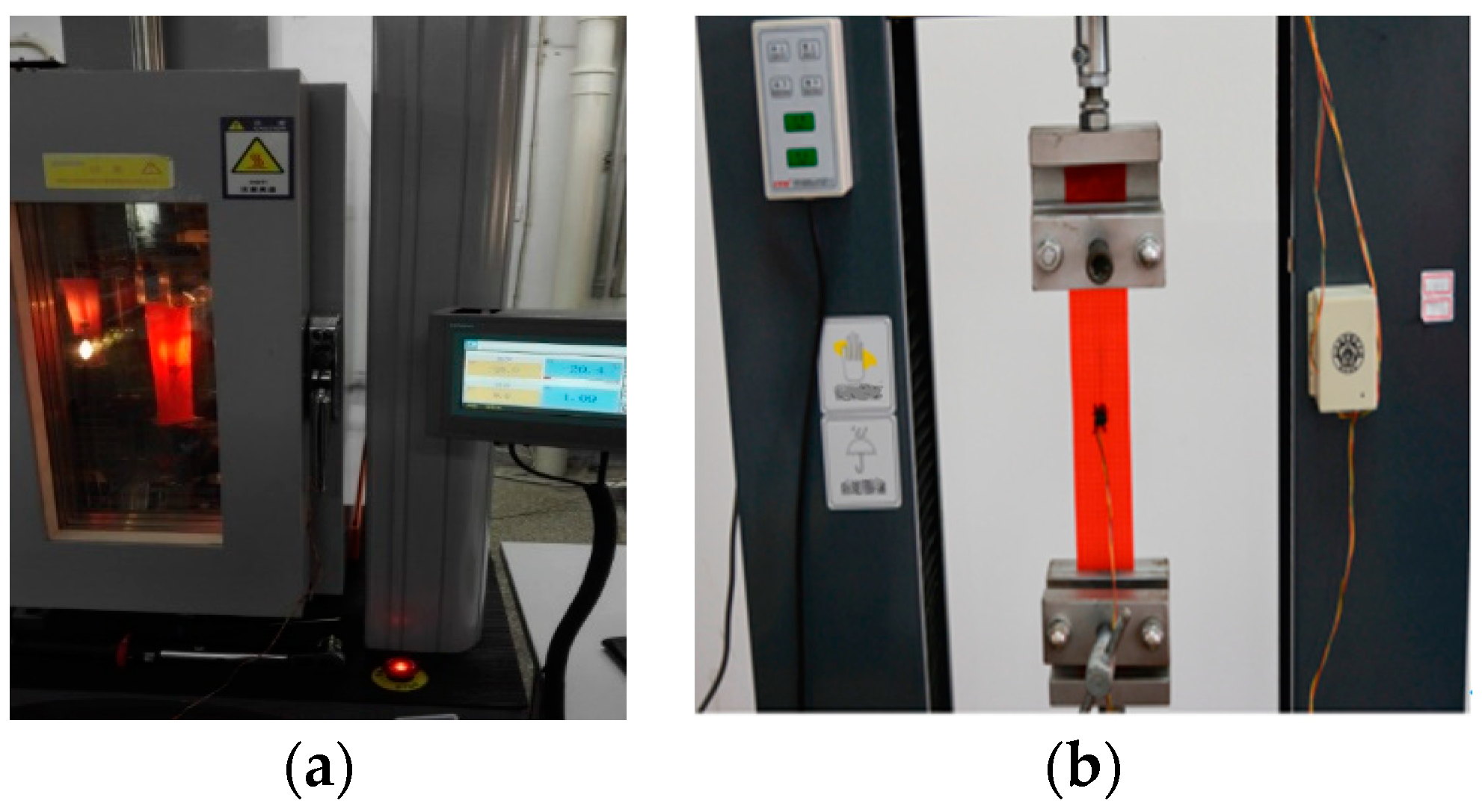
5.1. Model Training in THMTT Machine

In order to train the DC-BPNN model, we first perform experiments on the THMTT machine. The experimental environment is shown in the Figure 4, where the Ω-type sensor is fixed on the middle position of the 544-nylon-silk fabric (the same as parachutes’ fabric in our experiments) with the size 20 (cm) × 5 (cm). The sample fabric is placed on the machine, as shown in Figure 4a. The temperatures are respectively set as –25 °C, 0 °C, 20 °C, and 70 °C. Relative humidity values of each temperature are respectively set as 40%, 60%, and 80%. The stretching speed is set to 100 mm/min and the stretching range is 0 N to 200 N.

Basically, the $\Omega$-type on-chip sensor is based on the stress effect. When the conductor or semiconductor material has mechanical deformation under the influence of external force, its resistance value will change. Due to the difference in the sensitivity coefficient of the constantan material and the electrical resistivity, in the temperature of 20 °C, we find that the range of the sensitivity coefficient is 1.9–2.1 and the range of the resistivity range is 0.25–0.45 μΩ·mm. Therefore, different sensors measure distinct output voltages under the same stress.

Then, we establish the mapping between the stress and the output voltage through the THMTT machine experiments. The voltage, temperature and humidity are considered as the input of the training phase of DC-BPNN. We imitate the normal environment and set the standard output condition as the voltage of the same stress in 20 °C temperature and 40% humidity. We use the Cross-validation to set the parameters from multiple experiments: the number of neurons in the hidden layer is 20, and the maximum number of iterations is 50 of the Equation (2) to Equation (6), and the population size of AABC is 25, and the number of iteration limits of a single bee is 30 of the Equation (11) to Equation (13).

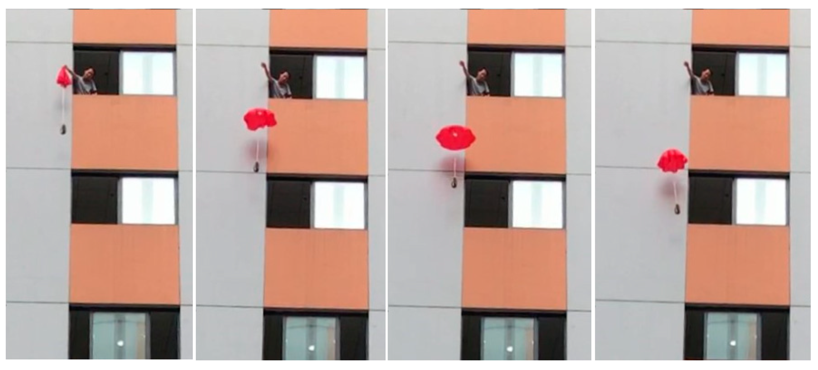
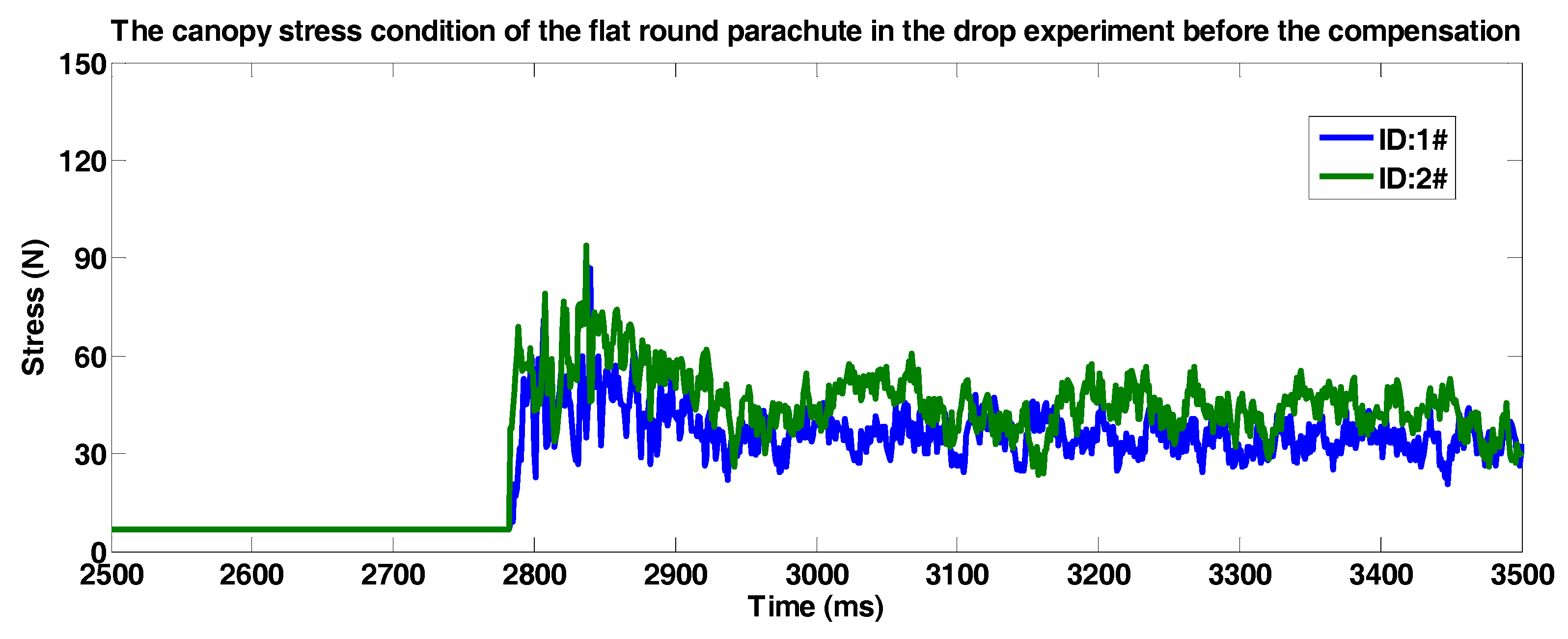
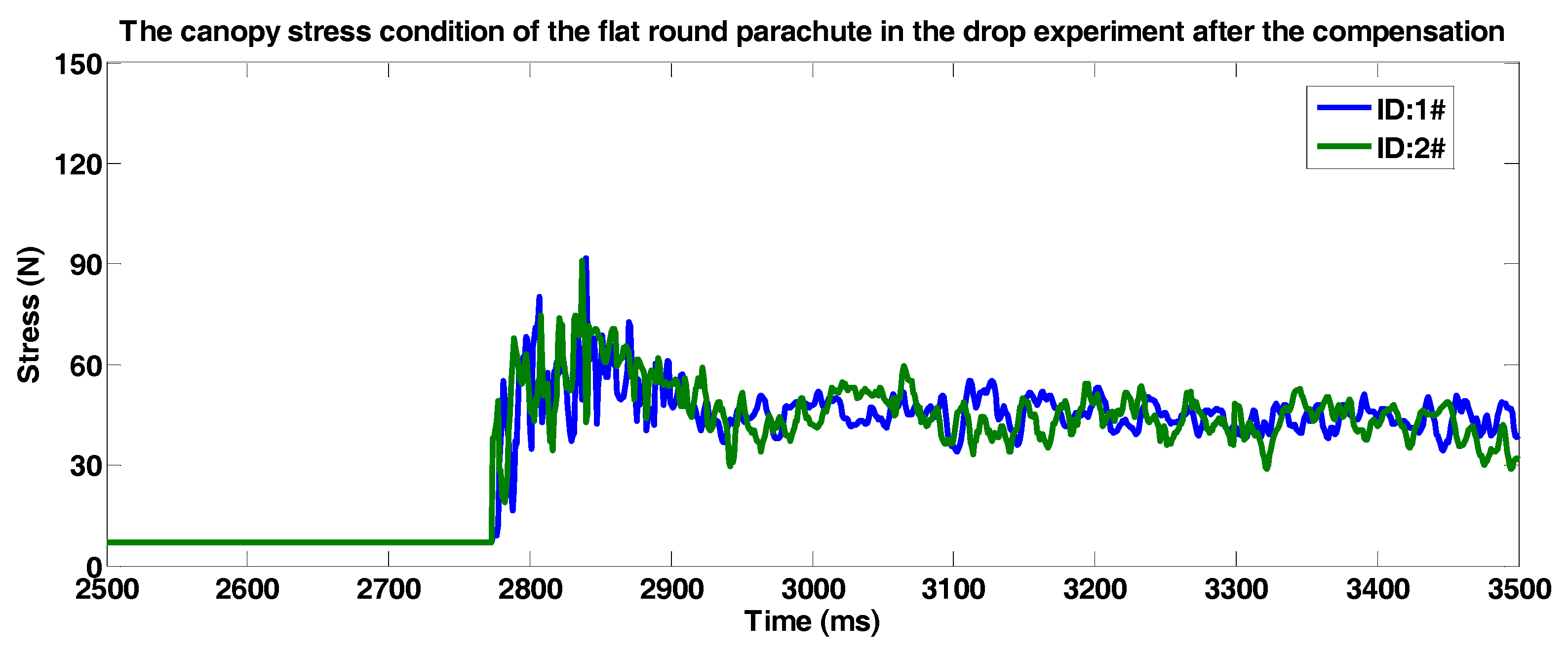
5.2. Airdropped Experiment

In this experiment, we deploy two sensors ID1 # and ID2 # on a parachute. Figure 5 shows the experimental environment. The drop height is about 15 m, and the load weight under the parachute is 2.5 kg. The temperature is 39 °C and the humidity is 76%. The horizontal wind speed is less than 0.2 m/s.

Figure 6 presents the stress data before compensation within 1000 ms after opening the parachute. For convenience comparison, the stress value on the base measured voltage was calculated. The instantaneous stress of the canopy reaches at a peak at the time about 2800 ms that the parachute ejects from the parachute pack. In the process of opening, the stress reaches maximum at about 2840 ms. The stress peaks of sensors ID1# and ID2# at the same latitude are 87.2.5 N and 91.6 N. Later, the stress weakens and keeps more stable during the airdrop process. Figure 7 shows the data after compensated, as we can see, as long as the stresses of two sensors are closer, the curves become smoother.

5.3. Effectiveness of AABC

We compare LM, ABC and AABC. The experimental results are shown in

Table 3. Comparison results of AABC, ABC and LM.

Methods	MSE			Time
	Optimal Solution	Average Value	Variance	Average (s)	Variance
LM	2.13 × 10−9	2.31 × 10−8	2.56 × 10−8	2.49	0.0224
ABC	2.23 × 10−10	2.91 × 10−9	2.87 × 10−9	2.29	0.0337
AABC	4.79 × 10−13	4.17 × 10−12	2.35 × 10−12	2.11	0.0646

. The parameters of ABC are set as same as AABC’s. The parameters of LM are set according to literature [34]. For each experiment, we select 12 different sets environmental conditions (all combinations of 4 different temperatures and 3 different humidity conditions), thus, we have 600 sets of data. We perform the experiment for 20 times and record the optimal value. From the Table 3, we can see that AABC algorithm can quickly find the optimal food source area, while the optimal solution value is smaller than the values in ABC and LM. AABC also has the advantage on running time. Therefore, compared with LM and ABC, AABC has faster convergence speed and global search ability, which can greatly improve the measurement accuracy.

6. Conclusions and Future Work

This paper presents DC-BPNN model for dynamic stress measurement with data compensation in an airdrop-deployed WSN. For optimizing DC-BPNN more effectively, a novel heuristic algorithm AABC is also proposed. In addition, to verify the effective performance, we use real deployed parachutes to present a set of measurement cases. The experimental results show that DC-BPNN with AABC provides efficiently compensation for sensor data. In our future work, we plan to deploy DC-BPNN in higher altitude space under various more complex conditions. Moreover, we will develop the system for huge parachutes for spacecraft.

References

1. Wu, S.; Niu, J.; Chou, W.; Guizani, M. Delay-Aware Energy Optimization for Flooding in Duty-Cycled Wireless Sensor Networks. IEEE Trans. Wirel. Commun. 2016, 15, 8449–8462. [Google Scholar] [CrossRef]
2. Xiao, Y.; Rayi, V.; Sun, B.; Du, X.; Hu, F.; Galloway, M. A Survey of Key Management Schemes in Wireless Sensor Networks. J. Comput. Commun. 2007, 30, 2314–2341. [Google Scholar] [CrossRef]
3. Liu, G.J.; Tan, R.; Zhou, R.; Xing, G.L.; Song, W.Z.; Lees, J.M. Volcanic Earthquake Timing using Wireless Sensor Networks. In Proceedings of the 12th ACM/IEEE Conference on Information Processing in Sensor Networks (IPSN), Philadelphia, PA, USA, 8–11 April 2013; pp. 91–102. [Google Scholar]
4. Du, X.; Xiao, Y.; Guizani, M.; Chen, H.H. An Effective Key Management Scheme for Heterogeneous Sensor Networks. Ad Hoc Netw. 2007, 5, 24–34. [Google Scholar] [CrossRef]
5. Giggenbach, D.; Epple, B.; Horwath, J.; Moll, F. Optical Satellite Downlinks to Optical Ground Stations and High-Altitude Platforms. Lect. Notes Electr. Eng. 2008, 16, 331–349. [Google Scholar] [CrossRef]
6. Zhao, J.; Zhuang, Y.; Gu, J.; Xu, Y.; Sun, J. Sensor Module Based on the Wireless Sensor Network for the Dynamic Stress on the Flexible Object with Large Deformation. J. Sens. 2016, 2016, 1–11. [Google Scholar] [CrossRef]
7. Motz, M.; Ausserlechner, U.; Holliber, M. Compensation of Mechanical Stress-Induced Drift of Bandgap References with On-Chip Stress Sensor. IEEE Sens. J. 2015, 15, 5115–5121. [Google Scholar] [CrossRef]
8. Deng, C.; Mao, Y.; Ren, G. MEMS Inertial Sensors-Based Multi-Loop Control Enhanced by Disturbance Observation and Compensation for Fast Steering Mirror System. Sensors 2016, 16, 1920. [Google Scholar] [CrossRef] [PubMed]
9. Xie, F.; Weiss, R.; Weigel, R. Hysteresis Compensation Method for Magnetoresistive Sensors Based on Single Polar Controlled Magnetic Field Pulses. IEEE Trans. Ind. Electron. 2017, 64, 710–716. [Google Scholar] [CrossRef]
10. Matko, V.; Milanović, M. High-Precision Hysteresis Sensing of the Quartz Crystal Inductance-to-Frequency Converter. Sensors 2016, 16, 995. [Google Scholar] [CrossRef]
11. Matko, V. Next Generation AT-Cut Quartz Crystal Sensing Devices. Sensors 2011, 11, 4474–4482. [Google Scholar] [CrossRef] [Green Version]
12. Xu, M.; Han, T.; Lin, Z. Energy-Efficient Time Synchronization in Wireless Sensor Networks via Temperature-Aware Compensation. ACM Trans. Sens. Netw. 2016, 12, 1–29. [Google Scholar] [CrossRef]
13. Verma, M.; Asmita, S.; Shukla, K. A Regularized Ensemble of Classifiers for Sensor Drift Compensation. IEEE Sens. J. 2016, 16, 1310–1318. [Google Scholar] [CrossRef]
14. Li, Z.; Zhao, X. BP artificial neural network based wave front correction for sensor-less free space optics communication. Opt. Commun. 2017, 385, 219–228. [Google Scholar] [CrossRef]
15. Liu, S.; Hou, Z.; Yin, C. Data-Driven Modeling for UGI Gasification Processes via an Enhanced Genetic BP Neural Network with Link Switches. IEEE Trans. Neural Netw. Learn. Syst. 2016, 27, 1–12. [Google Scholar] [CrossRef] [PubMed]
16. Karaboga, D.; Basturk, B. A powerful and efficient algorithm for numerical function optimization: Artificial bee colony (ABC) algorithm. J. Glob. Optim. 2007, 39, 459–471. [Google Scholar] [CrossRef]
17. Xu, Y.; Gao, F.; Ren, H.; Zhang, Z.; Jiang, X. An Iterative Distortion Compensation Algorithm for Camera Calibration Based on Phase Target. Sensors 2017, 17, 1188. [Google Scholar] [CrossRef] [PubMed]
18. Zheng, Y.; Wu, J.; Yang, Y. Temperature compensation of eddy current sensor based on temperature-voltage model. In Proceedings of the 12th World Congress on Intelligent Control. and Automation (WCICA), Guilin, China, 12 June 2016; pp. 438–441. [Google Scholar]
19. Bu, X.; Wu, X.; Wei, D.; Huang, J. Neural-approximation-based robust adaptive control of flexible air-breathing hypersonic vehicles with parametric uncertainties and control input constraints. Inf. Sci. 2016, 346, 29–43. [Google Scholar] [CrossRef]
20. Wei, P.; Cheng, C.; Liu, T. A Photonic Transducer based Optical Current Sensor using Back-Propagation Neural Network. IEEE Photon. Technol. Lett. 2016, 28, 1513–1516. [Google Scholar] [CrossRef]
21. Chen, X.; Zhang, M.; Ruan, K. A Ranging Model Based on BP Neural Network. Intell. Autom. Soft Comput. 2016, 22, 325–329. [Google Scholar] [CrossRef]
22. Kirkpatrick, S.; Gelatt, C.; Vecchi, M. Optimization by Simulated Annealing. Read. Comput. Vis. 1987, 220, 606–615. [Google Scholar]
23. Deb, K.; Pratap, A.; Agarwal, S.; Meyarivan, T. A fast and elitist multiobjective genetic algorithm: NSGA-II. IEEE Trans. Evol. Comput. 2002, 6, 182–197. [Google Scholar] [CrossRef] [Green Version]
24. Dorigo, M.; Birattrai, M.; Stutzle, T. Ant colony optimization. IEEE Comput. Intell. Mag. 2006, 1, 28–39. [Google Scholar] [CrossRef]
25. Kennedy, J.; Eberhart, R. Particle Swarm Optimization. In Encyclopedia of Machine Learning; Springer: Boston, MA, USA, 2011; Volume 4, pp. 760–766. [Google Scholar]
26. Chakrabarti, A. Mass-Spring-Damper System as the Mathematical Model for the Pattern of Sand Movement for an Eroding Beach Around Digha, West Bengal, India. J. Sediment. Res. 1977, 47, 311–330. [Google Scholar] [CrossRef]
27. Meng, J.C.S.; Thomson, J.A.L. Numerical studies of some non-linear hydrodynamic problems by discrete vortex element methods. J. Fluid Mech. 1978, 84, 433–453. [Google Scholar] [CrossRef]
28. Du, X.; Guizani, M.; Xiao, Y.; Chen, H.H. Transactions papers, A Routing-Driven Elliptic Curve Cryptography based Key Management Scheme for Heterogeneous Sensor Networks. IEEE Trans. Wirel. Commun. 2009, 8, 1223–1229. [Google Scholar] [CrossRef]
29. Jalalifar, M.; Byun, G. A Wide Range CMOS Temperature Sensor with Process Variation Compensation for On-Chip Monitoring. IEEE Sens. J. 2016, 16, 5536–5542. [Google Scholar] [CrossRef]
30. Gibbs, M.N.; Mackay, D.C. Variational Gaussian process classifiers. IEEE Trans. Neural Netw. 2002, 11, 1458–1464. [Google Scholar]
31. Bousquet, O.; Elisseeff, A. Stability and generalization. J. Mach. Learn. Res. 2002, 2, 499–526. [Google Scholar]
32. Hardt, M.; Recht, B.; Singer, Y. Train faster, generalize better: Stability of stochastic gradient descent. Int. Conf. Mach. Learn. 2016, Jun 11, 1225–1234. [Google Scholar]
33. Shalev-Shwartz, S.; Shamir, O.; Srebro, N.; Sridharan, K. Learnability, stability and uniform convergence. J. Mach. Learn. Res. 2010, 11, 2635–2670. [Google Scholar]
34. Budil, D.E.; Lee, S.; Saxena, S.; Freed, J.H. Nonlinear-Least-Squares Analysis of Slow-Motion EPR Spectra in One and Two Dimensions Using a Modified Levenberg–Marquardt Algorithm. J. Magn. Reson. Ser. A 1996, 120, 155–189. [Google Scholar] [CrossRef]
Figure 1. Structure of dynamic measurement system based on airdropped WSN. (a) Overall system structure. (b) Deployment detail on a parachute.
Electronics 08 00859 g001
Figure 2. Data acquisition and transmission.
Electronics 08 00859 g002
Figure 3. WSN acquisition data compensation framework.
Electronics 08 00859 g003
Figure 4. Experiments in THMTT machine. (a) Overall structure of the machine. (b) Core part of the testing machine.
Electronics 08 00859 g004
Figure 5. The opening process of the parachute in the airdropped experiment.
Electronics 08 00859 g005
Figure 6. The canopy stress condition of the flat round parachute before the compensation.
Electronics 08 00859 g006
Figure 7. The canopy stress condition of the flat round parachute after the compensation.
Electronics 08 00859 g007